In the digital video broadcasting satellite services to handhelds (DVB-SH) system for ... media data is thus buffered at the client side until all interleaved data or redundancies are ... affordable overhead for upper layer FEC redundancy is usually small. ... this reason, the tradeoff between the FEC recovery requirement and the ...
◆
Variable FEC Decoding Delay and Playout Slowdown Method for Low Start Delay and Fast Channel Change for Video Streaming in DVB-SH Mobile Broadcast Systems Frédéric Faucheux, Marie-Line Alberi Morel, Sylvaine Kerboeuf, and Laurent Roullet In the digital video broadcasting satellite services to handhelds (DVB-SH) system for broadcasting multimedia services to mobile receivers, a multiprotocol-encapsulation inter-burst forward error correction (MPEIFEC) technique has been introduced to mitigate the deep signal fading events which primarily occur in the land-mobile satellite channel. It is based on a clever organization of data and parities with long interleaving. The media data is thus buffered at the client side until all interleaved data or redundancies are received before decoding begins. The more the data is protected against loss, the more video impairment decreases and latency increases. Latency negatively impacts the playout start time and switching time. A tradeoff is usually necessary between the video quality and the forward error correction (FEC) decoding latency. Such a tradeoff is realized in a static mode. Alternatively, in this paper we investigate how an adaptive media playout and variable FEC decoding delay scheme can provide low latency while providing good video quality. We then evaluate user quality of experience when the method is used in DVB-SH broadcast networks. © 2012 Alcatel-Lucent.
Introduction Video consumption is becoming a part of our daily life. Nielsen reports that U.S. broadcast television (TV) viewership in 2011 reached 158 hours 47 minutes a month while mobile viewership increased 20 percent over one year with video consumption of 4 hours 20 minutes a month in first quarter 2011 [14]. Video services delivery including video streaming will soon represent the majority of Internet traffic. In addition, video on demand or live TV services on mobile
devices such as smartphones are becoming key services in wireless networks. However, media streaming over the Internet or over Internet Protocol (IP) packet-based wireless networks is sensitive to packet loss which impacts the quality of experience for the end user. Indeed, packet loss can cause errors or even interruption in video playout. This problem is even more drastic for media streaming over mobile broadcast communication systems such as in digital
Bell Labs Technical Journal 16(4), 63–84 (2012) © 2012 Alcatel-Lucent. • DOI: 10.1002/bltj.20534
Panel 1. Abbreviations, Acronyms, and Terms 3GPP—3rd Generation Partnership Project ADST—Application data sub-table ADT—Application data table AMP—Adaptive media playout AVC—Advanced video coding DVB—Digital video broadcasting DVB-H—DVB-handheld EM—Encoding/decoding matrices eMBMS—Enhanced multimedia broadcast/multicast service FDT—FEC data table FEC—Forward error correction fps—Frames per second GOP—Group of pictures IFEC—Inter-burst forward error correction IP—Internet Protocol IPTV—Internet Protocol television ITS—Intermediate tree shadowed
video broadcasting satellite services to handhelds (DVB-SH) [8]. In DVB-SH, deep signal fading events over the land-mobile satellite channel can cause bursts of packet loss of lengthy duration. In order to recover from this loss, forward error correction (FEC) techniques can be used when, for example, retransmission is not possible because of the broadcast system, e.g., 3rd Generation Partnership Project (3GPP), (Enhanced) Multimedia Broadcast/ Multicast Service ((e)MBMS), Digital Video Broadcasting-Handheld (DVB-H)/Satellite Services to Handhelds (SH)/NextGeneration Handheld (NGH). The upper layer FEC codes add redundant information to the original data flow, which can be used by the receiver to reconstruct the erased data, e.g., packets lost by a congested router or errors over a wireless link [13]. These codes are usually designed with a high code rate since the affordable overhead for upper layer FEC redundancy is usually small. In addition, a time interleaving technique is thus used to increase the robustness against losses. The FEC/interleaver is usually designed to cope with the worst case of channel losses. The coded/ interleaved data spans a long time duration to provide enough correction efficiency. In the end, these
64
Bell Labs Technical Journal
DOI: 10.1002/bltj
LDPC—Low-density parity-check LMS—Land mobile satellite MPE—Multi-protocol-encapsulation NDK—Native development kit NGH—Next-generation handheld QoE—Quality of experience QPSK—Quadrature phase shift keying RFR—Recovery failure rate RR—Recovery rate RS—Reed-Solomon RTP—Real Time Transport Protocol SH—Satellite services to handhelds SUB—Suburban TV—Television TVMSL—Télévision Mobile Sans Limite UDP—User Datagram Protocol WSOLA—Waveform-singularity-based synchronized overlap-add
FEC and interleaving techniques result in the introduction of an additional latency at the receiver side because it is necessary for the receiver to wait long enough for the reception of all interleaved data and/or FEC redundancy. The more the data is protected against loss, the more video impairment decreases and latency increases. Thus, the FEC decoder latency negatively impacts the total latency resulting in a longer playout start time and channel switching time. For this reason, the tradeoff between the FEC recovery requirement and the latency is usually an important part of system design. To ensure rapid start and fast channel changes, the delay before decoding at FEC decoder must be set to a minimum value obtained from a tradeoff against the resulting video quality, as studied in [2]. When the FEC decoding delay is reduced to favor a low-delay media playout start, it is done at the cost of possible degradation in video quality since the FEC decoding will be processed before all necessary source and redundancy data are received. It is not possible to get good video quality in conjunction with low FEC decoding latency, and thereby a short delay before playout. Note that the playout start occurs not just at power-up
but whenever the signal is lost due to long fade times that exceed the code capacity such as those from tunnels or “truck fades.” To address this problem, in this paper we investigate how an adaptive media playout and variable FEC decoding delay scheme can provide short latency while providing good video quality. Adaptive media playout (AMP) is a well-known technique investigated in [12], and more recently in [3] and [20], that consists of adapting the playout speed of the video to control the client buffer in order to absorb the network jitter and avoid interruption in the video playout. In this study, the AMP is used to cope with a variable FEC decoding delay. The paper is organized as follows. First, the variable FEC decoding delay method is investigated with respect to short playout start time. The adaptive media playout is then introduced and the resulting requirements in the architecture of the client are discussed. Second, the impact of this approach on the video quality is analyzed. For this, we consider a Multi Protocol Encapsulation Inter-Burst Forward Error Correction (MPE-IFEC) scheme for video streaming over a DVB-SH broadcast network that integrates the variable FEC decoding delay. The decoding performance of the MPE-IFEC decoder is derived analytically in terms of the probability of recovering a lost datagram burst. This statistical performance model is thus used to analyze the achievable video quality just after a start or a channel change. Third, comparisons with experimental results show the improvement brought by the suggested approach in terms of the reduction of non-displayable frames. Finally, we draw some conclusions.
Variable FEC Decoding Delay Approach and Adaptive Media Playout Forward error correction codes add redundant information to the original data flow, which can be used by the receiver for reconstructing the erroneous or erased data. FEC codes introduce a delay which can be reduced by using a variable FEC decoding delay approach, which implies using an adaptive media playout.
FEC Technique and Latency at FEC Decoder In many media streaming systems, upper layer FEC (i.e., any FEC code operating above the physical layer at the link or application layer using erasure decoding) is proposed to overcome the losses resistant to physical layer FEC mechanisms, and link layer retransmission schemes [6]. An FEC encoder generates n encoding symbols from k source symbols. A symbol could consist of, e.g., a bit, a byte, or a packet of data. The FEC block size is defined as the number of source symbols which are protected together. The code rate is defined as the ratio k/n. The FEC overhead refers to the additional FEC data (the number of redundancy packets) as a fraction of the source data, (n � k)/k. The FEC techniques are opposed to repeat request techniques whereby the receiver asks for the retransmission of lost symbols. Physical layer FEC codes work at the bit level and are traditionally implemented as part of the radio interface for broadcast wireless communication systems. Upper layer FEC operates with large blocks of source packets which introduce a delay while the FEC decoder needs to wait before processing the received data. The Raptor, LowDensity Parity Check (LDPC), and Reed-Solomon codes are the most popular schemes proposed in the literature [11, 16, 19]. FEC is usually designed to cope with the worst case of channel packet loss. This determines the amount of redundancy needed to recover all possible loss. It is worth noting that such media systems can only be optimized by taking into account the overall correction capacity of both physical and upper layer FEC within the total bandwidth overhead budget, which is limited by the system. The affordable overhead for upper layer FEC code correction is usually very low. However, upper layer FEC is generally combined with a time interleaving technique to increase the robustness against loss. This is due to the fact that the packet losses over a land mobile satellite (LMS) transmission channel are correlated, and occur in long bursts lasting several seconds. Permuting a sequence of bits in the coded data before their transmission distributes the coded data over time, so that errors in the interleaved coded data are more uniformly distributed in time after de-interleaving, and therefore easier to correct with FEC codes [4]. The interleaving
DOI: 10.1002/bltj
Bell Labs Technical Journal
65
of coded data over a long time duration improves the FEC correction efficiency without increasing the bandwidth overhead, but this increases the additional delay the FEC decoder/de-interleaver needs to wait before processing the received data and thus delivers them to the upper layer. In the following, we define the FEC decoding delay at the FEC decoder as the period of time elapsed between the reception of the coded data and the FEC decoding/de-interleaving operation. During this buffering delay, additive data and FEC information are collected by the decoder to proceed to the decoding of the current data burst once all the parities have been received. A generic model of the systematic encoding and decoding process is shown in Figure 1. In this model, it
Data
Delay
Data
can be seen that the FEC encoding process (Figure 1a) induces two types of delays on the decoding side: • One in relation to the interleaving depth of the generated parity (“FEC interleaving delay”), and • One in relation to the depth of the data interleaving (“data interleaving delay”). On the decoding side (Figure 1b), a decoding with full protection can occur when all interdependent data and FEC have been received. In the literature, this state is referred to as “late decoding” [10]. The term “late” is used because received data must be delayed before it can benefit from decoding. This is due to the interleaving done at encoding that requires a reciprocal de-interleaving. The delay function depends on the type of encoding (block, convolutional) and the scope
Data
Data
MUX
Data storage
Data
Data Data interleaving
Data encoding
Data interleaving delay
FEC
FEC interleaving
FEC
⫹ FEC
FEC interleaving delay
(a) Encoder generic architecture
DEMUX
⫹
Data
Data
Data
Data delay
Da FEC
Selection
FEC Da FEC Data and FEC storage
Data and FEC de interleaving
Data FEC Data decoding
(b) Decoder generic architecture FEC—Forward error correction
Figure 1. Generic encoding and decoding processes.
66
Bell Labs Technical Journal
DOI: 10.1002/bltj
Data
Data
(how many blocks of data are involved in the encoding process). However data may be displayable much earlier, this is called “early decoding”: • This early decoding state is possible when data is sent with its own correction capability, usually called the “inner FEC” (not illustrated in Figure 1) and when a second “outer FEC” (illustrated in Figure 1) is added “on top” of an existing “inner” protection scheme. Usually the “outer FEC” provides an additional protection level while not impacting existing mechanisms using the “inner FEC.” The inner FEC is applied after the outer FEC, more precisely, after the MUX function in the encoder generic architecture and before the DEMUX function in the decoder architecture. • If reception conditions are good, the receiver does not need to wait for other remaining data and/or for the remaining “outer FEC” to display since it can rely on the inner FEC. Relying on only the inner FEC obviously comes at the price of lower robustness. • In the decoder, this state corresponds to the reception of the data on the top path, excluding any data coming from the lower path. In such early decoding, the data delay function can be set to zero since the selection block does not need to wait for the decoding of the lower path. The possibility of early decoding makes the following features possible: • More flexibility (within the total available bit rate) in terms of code rate, interleaving, and type of FEC code is therefore possible for the “outer FEC.” Otherwise and without the early decoding, most of the protection would need to go to the shorter FEC to respect minimal zapping time delays which would in turn call for a unique FEC. Since early decoding relaxes the interleaving duration constraints, it is possible to split FEC into several types, each having its own encoding FEC, interleaving depth, and code rate. • Outer FEC interleaving data depth may be significantly increased compared to the “inner FEC” in ratios proportional to the outer FEC code rate. For a given level of robustness, the FEC code rate will vary proportionally with the interleaver
duration since the longer the interleaver, the better the protection and the higher the required code rate. Thus early decoding is a nice technique when combined with split FEC situations. However its usage requires adaptive media playout in order to recover this depth and reach “late decoding” state. In the following, we focus on the model for an outer FEC decoder. For simplicity, we will refer to it as the “FEC decoder.” Note that inner and outer FEC usually refers to the channel (or physical) and link (or upper) FEC but this is not always the case. Many variations are possible. For instance, it is possible to use complementary turbo codes at the physical layer, or incremental redundancy with LDPC, or complementary Raptor codes at the upper layer. So the inner and outer FEC terminology can be used in a wide scope even if we provide results here only for the first case. Variable Decoding Delay at FEC Decoder The delay introduced at the FEC decoder can be too long to provide a satisfying quality of experience for the viewer when starting the program playout and upon a program or TV channel change request, or after a long period without receiving a signal, as when emerging from a long tunnel. On the receiver side, to obtain maximum protection, all data and the corresponding parities must be received before proceeding to the FEC decoding. This operating mode, which is called the late decoding mode, leads to optimal performance; however it comes at the cost of increased receiver latency and delay at start-up or channel change. To reduce this latency, an alternative mode of decoding, referred to as the early decoding technique, is defined for the FEC decoder. In this mode, the data bursts received are delivered to the upper layers without waiting for reception of all data and parity. Early decoding mode reduces the FEC decoding delay before the datagram burst decoding. For rapid start or fast channel changes, the FEC decoding delay requirement must be set to a minimum value obtained by a tradeoff with the resulting video quality, as studied in [2]. However the maximal correction capacity is never reached after the channel change at the decreased decoding time. If errors occur, DOI: 10.1002/bltj
Bell Labs Technical Journal
67
data is decoded by FEC with a reduced correction capacity that leads to video quality degradation. On one hand, the technique for fast playout start relies on the early decoding approach. On the other hand, the technique for having a good video quality relies on the late decoding mode with the maximum correction capacity (using the FEC mechanism). Our goal is thus to find a way to take advantage of these two techniques in spite of the fact that they are opposed. To solve the tradeoff issue between video quality and low latency, we thus propose to design an FEC decoder with a variable decoding delay. The FEC decoder starts to decode the first data received (source � redundancy) without waiting to receive all the required redundancy data, i.e., a low value is set for the initial FEC decoding delay. This allows for a rapid start of the video playout. Then, the FEC decoder progressively increases its decoding delay until complete recovery can be realized before outputting the data. This achieves an FEC decoding delay which offers maximum protection against loss as well as good overall video quality. From this instant FEC operates in a mode referred to as late decoding mode in which data is corrected with all parities. Such a mechanism can be run not only at start time, but also every time a playout interruption occurs to ensure a fast restart. The variable FEC decoding delay can potentially be applied to upper layer FEC mechanism introduced in many current standardized media streaming systems, e.g., 3GPP/MBMS [1], DVB-SH [10], DVB-Internet Protocol television (IPTV) [9] to reduce the playout (re)start delay if necessary. Adaptive Media Playout The variable FEC decoding delay will impact the rendering of the media playout. It introduces jitter in the output data (i.e., frames data) provided to the media player buffer. Once started, the media player must display the frames at a regular media frame rate otherwise the playout is jerky or even frozen. This situation is quite similar to the problem of reception buffer filling for video streaming over a rate-changing medium, for which the solution of adaptive media playout has been proposed [3, 12, 20]. The adaptive media playout technique consists of adapting the
68
Bell Labs Technical Journal
DOI: 10.1002/bltj
media playout speed to compensate for network fluctuations. Increases or decreases in the playout speed are expected to be the least bothersome solution to the viewer instead of experiencing playout jerkiness or interruption. AMP also serves to reduce the start time by permitting a lower initial buffering, the buffering being progressively increased to the nominal target with respect to network conditions thanks to a lower playout speed (e.g., playing the video at 20 frames per second (fps) instead of 25 fps). From the experimental tests done by our team, it appears that the useful range for modified playback rate scales from 70 percent to 150 percent. It actually depends a lot on the video content (in a fast moving scene a slowdown is more easily noticed), audio content (a slowdown of music is more noticeable than a slowdown of speech, because of the tempo change) and the end user’s attentiveness to the content. In our case, in which variable FEC decoding delay is used to ensure a fast start, the video playout speed is uniformly slowed down while at the same time FEC decoding delay is uniformly increased in order to provide a jitter-free buffer at the video player level. The slowdown occurs during the transition period while the decoding delay is progressively increased. Then it returns to the normal playout speed when the decoding delay reaches the value for having a maximum error correction power. This is called the steady state, and it is illustrated in Figure 2. The slowdown ratio of the playout speed, referred to as a is defined as the ratio of displayed frames per second during the transition mode (fpsout) to original frames per second (fpsin ), a�
fpsout fpsin
(1)
Optimal FEC Decoding Delay Variation Rate Versus Playout Speed The FEC decoder outputs the first data packet after a buffering time delaymin and the subsequent packets on a regular basis in time with respect to the media playout. If we neglect the durations of the video decoding and the time needed for display, delaymin corresponds to the playout start time or channel change time duration. When media slowdown is realized with ratio a, the decoding delay at the FEC decoder for the
Displayed frame ID
4500
o o++ o+o+ + o Fast channel switching + +o+ +o 4000 o+o Late decoding mode o + o o ++ o +o+ o o + + 3500 oo o+ ++ o + o + +o oo ++ 3000 + oo + o + oo o+ o+ + + o +o 2500 o+o + +o+o + o o o+ Transition period o+ ++ 2000 o + o + o Steady state ++o ++ oo ++oo + + o 1500 ++ o ++ooo + ++ o ++ oo 1000 ++ ooo + + o ++ o ++ ooo + o ++ 500 ++ ooo ++ o + + oo ++ oo 0 ++ 0 20 40 60 80 100 120 140 160 180 Time after switching channel
ID—Identifier
Figure 2. Slowdown and steady state.
current packet n is given by dn � tn,out �tn,in, the time elapsed between the reception time of the data for the nth received packet tn,in and its decoding time tn,out and is expressed as: dn � a
1 � 1b � (tn,in � t0,in ) � delaymin a
(2)
where t0,in is the reception time of the first data packet. This equation shows that the decoding delay increases linearly with the relative reception time during the transition period. The entrance of the decoder in the steady state marks the end of the transition period. At this time, the delay to decode the current packet with respect to its reception time corresponds to the delay for having received all data and parity concerning the packet and is denoted by delaymax. Using equation 2, the elapsed time between the reception time of the first data packet and the instant when dn reaches the value delaymax is expressed as,
decoder ¢t transient � (delaymax � delaymin) �
a 1�a
(3)
The duration perceived by the viewer of the transient period is then expressed as display ¢t transient � delaymin �(delaymax � delaymin) �
a (4) 1�a
This duration indicates the delay between the first data received by the decoder (close to the channel join request or service start instant) and the time when the correction capacity of the system reaches its maximum level, which also marks the end of the slowed down playout (AMP). Receiver Architecture The proposed architecture for the receiver is illustrated in Figure 3. Due to the particular nature of real time multimedia streams, the AMP mechanism results in a need to modify the actual content of the payload; this is done in a module called AMP controller,
DOI: 10.1002/bltj
Bell Labs Technical Journal
69
Control link: slowdown rate ⫽ α Value of α
IP packets
FEC decoder ⫹ de-interleaver
AMP controller
Media player
Start/stop slowdown AMP—Adaptive media playout FEC—Forward error correction IP—Internet Protocol
Figure 3. Receiver architecture.
which can synchronize with the FEC decoder module and sends a modified stream to the video decoder module that should support some special requirements. FEC decoding and de-interleaving module. In the nominal case, this decoding occurs only when enough time has elapsed to have theoretically received all the parities for the relevant data packet. In the case of AMP, the FEC decoding occurs earlier depending on the values of delaymin and a. These parameters can be read from configuration files and/or they may be transmitted through a control link over the network. The important point is that the values must be shared by the FEC decoding module and the AMP controller. Upon reception of a packet, the FEC decoder calculates the delay dn after which the data should be output to the next module, using equation 2. The use of packet identifiers allows the detection of data losses. When a missing packet is detected, an empty packet is internally created with an estimated reception time that is then employed to calculate the delay dn using equation 2. At the expiration of this delay, both missing packets and packets with partial loss are reconstructed by the decoder which transmits the corrected packets (as long as the erasure rate 70
Bell Labs Technical Journal
DOI: 10.1002/bltj
does not exceed the capacity of the code to correct the incoming packet string). AMP controller. The role of this module is to modify a part of the data content in order to obtain a media stream in that is consistent with the slowdown of the decoding. One way to achieve this task is to analyze the stream at the container level and change the values of the listed timestamps, e.g., the timestamps of the Real Time Transport Protocol (RTP). If no modification is applied to these timestamps a problem may arise at the player level: due to the slowdown mechanism, the differences between the coded timestamp and the actual time will grow and the player will think the received packets are late and may decide to drop them. The formula used by the AMP controller to modify the timestamps is:
TS� �
TS �C a
(5)
Where: • TS is the initial timestamp value, equal to the number of clock ticks (the clock frequency value is transmitted in a control message),
•
TS’ is the modified timestamp value consistent with the slowed down playout, C is a constant defined as: 1 C � TS0 � a1� b � (delaymax � delaymin) � freqts a (6)
TS0 denotes the first timestamp information received after channel switching and freqts denotes the clock frequency of the timestamp. This modification should be done in the container, and if possible, also in the coded stream. C is calculated so that there is no discontinuity in the timestamp value when the system switches from transition period to steady state (even though timestamp discontinuity still occurs when a frame cannot be reconstructed). Video and audio issue. The following parameters have to be considered in order to estimate the viewer quality of experience in a solution using AMP: the elapsed delay between the new program or TV channel request and the beginning of the playout, the quality of the displayed video (few impaired frames), and the requirement that the slowdown remains unnoticeable to the viewer’s sight and hearing. Considering the video rendering, playing frames at a lower rate simply results in displaying each frame for a longer delay, which can remain unnoticed to the viewer. The audio level presents another problem: if the sample is played at its normal speed, the next sample will not be ready to play immediately after the current one is done, and silence will be heard between the two, resulting in noticeable “clicks” to the listener. The trivial time-scaling approach can solve this problem but it changes the frequency of the sample, producing a highly noticeable pitch difference even at 90 percent of the original speed. Fortunately, there are other algorithms such as waveform-singularity-based synchronized overlap-add (WSOLA), which are able to time scale audio samples without affecting the pitch [21]. Although the tempo is modified, it is a lot less noticeable and disturbing than a change in the pitch. The other problem is determining which module should take care of applying the algorithm. It is possible to do it at the AMP controller level, or in another special module between the AMP controller and the
player. In this case, the chosen module will have to decompress the audio sample, then modify it thanks to the said algorithm and finally re-encode it into the correct format. The drawback of this method is that it is complex and necessitates a transcoding of the audio, but the advantage is that it is compatible with all players. Another solution is to use a player which can do the modification itself. In this case only one decoding is needed, rather than two decoding phases and one encoding. This leads to better performance, but imposes more overhead, e.g., that the player supports this technique. Playback of slowed down audio is currently possible with both the iPhone* (using built-in features) and Android* phones (using the SonicNDK).
AMP and Variable FEC Decoding Delay: Impact on Video QoE for DVB-SH Systems We now consider the case when AMP and variable FEC decoding delay is applied to hybrid satellite/ terrestrial broadcast DVB-SH systems. The FEC technique introduced into the DVB-SH standard is a multi-protocol-encapsulation inter-burst forward error correction (MPE-IFEC) technique to mitigate deep signal fading events lasting up to several consecutive time sliced bursts on land mobile satellite channels [8]. It is based on a clever organization of data and parities offering long interleaving and long encoding. MPE-IFEC interleaves data over a long time before encoding. It interleaves the parity symbols produced to transmit them over the air while the data is transmitted non-interleaved. For example, data is sent in periodic bursts of about 1 second duration and the parity symbols are spread over several bursts. This results in the introduction of several seconds of latency at the decoding stage. MPE-IFEC Including the Variable Decoding Delay In this section we explain how MPE-IFEC achieves the specific interleaving of data and parity that is robust in shadowed environments [5, 18]. MPE-IFEC is a sliding encoding scheme based on parallel processing of M encoding/decoding matrices (EM) structured into one application data table (ADT) filled with IP data coming from a datagram burst, and one FEC data table (FDT) containing redundancy bytes. In fact, each datagram burst is first mapped DOI: 10.1002/bltj
Bell Labs Technical Journal
71
burst K. In the figure, the time sliced burst is labeled with the index of the datagram burst it carries. The previously introduced modes of early decoding and late decoding have been defined for MPEIFEC. In late decoding mode, MPE-IFEC waits for reception of all data and parity before data decoding with the maximal correction capacity. In early decoding mode, received data bursts are delivered to the upper layers without waiting for reception of all data and parity. Thus the latency introduced by the long interleaving of MPE-IFEC is decreased inducing a reduction of the channel change delay. However, the data signal is partially corrected by MPE-IFEC in the case of transmission errors since only a portion of the B ADT entities can be decoded with the received parity. Consequently, more errors could occur in displayed pictures using early decoding mode. The decoding time of MPE-IFEC is fixed by the parameter d. According to d, MPE-IFEC operates in an early or late decoding mode. It operates in the early decoding mode if d is lower than (B � S) when D � 0 or lower than B when D � B � S [2]. At the instant of channel change, MPE-IFEC operates in the early
onto an application data sub-table (ADST) matrix. The ADST matrix is split into B parts and each part is stored into one ADT. By applying the Reed-Solomon (255, 64) code on each row of the ADT, the generated redundancy bytes (also called sections) of MPE-IFEC are stored in the FDT. The parity symbols are thus produced by combining columns coming from B different datagram bursts [7]. The resulting parity is transmitted over S consecutive time sliced transmission bursts over the air whereas the original datagram burst is transmitted over one single time sliced burst. Because of the interleaving, current datagram burst K is decoded using data and parity spread over time sliced bursts. The transmission of IP data and parity symbols over the air is determined by the two schemes D � 0 (parity sent after data) and D � B � S (parity sent before data) illustrated in Figure 4. The parameter D represents the number of bursts during the time between the reception of the datagram burst from upper layers and its transmission over the air. Namely the datagram burst K-D and the MPE-IFEC burst K generated when the datagram burst K was received are transported over the air in the time sliced
D⫽0
FEC of datagram burst K carried over B⫹S⫺1 time-sliced bursts
...
K⫺B⫹1
...
K⫺1
K
K⫹1
...
K⫹B⫺1
...
K⫹B⫹S⫺1
...
t
2B–1 time-sliced bursts used in calculation of FEC of datagram burst K
D ⫽ B⫹S
FEC of datagram burst K carried over B⫹S⫺1 time-sliced bursts
...
K⫺B⫺S⫹1
...
K⫺B⫹1
...
K⫺1
K
K⫹1
...
K⫹B⫺1
2B–1 time-sliced bursts used in calculation of FEC of datagram burst K
FEC—Forward error correction
Figure 4. Time transmission schemes for D � 0 and for D � B � S.
72
Bell Labs Technical Journal
DOI: 10.1002/bltj
t
decoding mode with d � delaymin. During the transition period, d increases progressively from delaymin to a maximal value delaymax until MPE-IFEC enters the steady state. The value for delaymax is B � S when D � 0 and B when D � B � S.
to k � d. Therefore, the probability of recovering a lost datagram burst Dk, denoted by the error recovery rate (RR), is given by the following product: B�1 d RR � q p(EMm,k )
(7)
m�0
Burst Error Recovery Rate Versus MPE-IFEC Decoding Delay In this section, we derive the probability of recovery of a lost datagram burst. Denoting by Dk the datagram burst received during the kth period of service and by Dm,k the set of columns of Dk belonging to the mth encoding matrix, denoted by EMm,k with m � 0 . . . B � 1. Dk is split into B sub-blocks. The B sub-blocks fill B matrices among M matrices with respect to the convolutional interleaving method detailed in [2]. EMm,k is composed of two tables ADTm,k and FDTm,k thus composed by sub-blocks belonging to consecutive received datagram bursts, as illustrated in Figure 5. ADTm,k is filled with data sub-blocks from consecutive received datagram bursts such that ADTm,k � h 5Dj,k�m�j 6j�1. . . B. FDTm,k contains FEC subblocks such that FDTm,k � h 5Fl,k�m�1 6 l�1. . . S. A lost datagram burst Dk is recoverable if the set 5Dm,k 6 m�0 p B�1 is recoverable, i.e., if the B decoding matrices EM dm,k, that contain all the sub-blocks of Dk, are successfully decodable for a decoding time equal
Sub-block from the oldest datagram burst
D1,k⫹m⫺B
p(EMdm,k ) represents the probability of successfully decoding the mth decoding matrix EMdm,k. The event of correctly decoding each matrix EMdm,k is assumed to be independent. The decoding is achieved at different instants with different sets of data columns coming from different datagram bursts (convolutional interleaving). Applying an ideal Reed-Solomon (RS) code to each decoding matrix for correcting the data [8], p(EMdm,k ) depends on the correction capacity of RS code (Ca) and the number of columns that are involved in the computation of parity symbols of Dm,k and are not received by ADTm,k and by FDTm,k at the decoding instant k � d. The column losses are mainly caused by deep channel fading, but can also be caused by a decoding time that is too short in comparison to the time necessary for data (2B � 1) and parity (B � S � 1) interleaving, as shown in Figure 4. The fading causes random losses (erased columns) whereas the mismatch of decoding time causes determinist losses (columns declared lost) depending on d.
Sub-block from the most recent datagram burst
...
Dm,k
...
DB,k⫹m⫺1
The first transmitted FEC sub-block
F1,k⫹m⫹1
The last transmitted FEC sub-block
F2,k⫹m⫺1
ADTm,k
...
FS,k⫹m⫺1
FDTm,k
EMm,k ADT—Application data table EM—Encoding/decoding matrices FDT—FEC data table FEC—Forward error correction
Figure 5. Structure of the encoding matrix EMm,k containing the sub-block Dm,k and Fl,k�m�1.
DOI: 10.1002/bltj
Bell Labs Technical Journal
73
The number of erased columns is expressed as a function of the number of erased sub-blocks. The number of erased sub-blocks in ADTm,k and in FDTm,k is denoted respectively by the random variables Xm,k and Ym,k. They are assumed independent since they come from sub-blocks received from separate bursts that are assumed to be independently distributed [17]. Both tables, Xm,k and Ym,k are also assumed to be independently distributed. As a consequence, the probability of successfully decoding EMdm,k for a decoding time equal to k � d is equivalent to the probability of getting a number of erased sub-blocks in FDTm,k less than the bound S � hYm,k (d) � W(x) knowing that ADTm,k exhibits a number of erased sub-blocks equal to the variable x. This bound determines the maximal number of erased FEC sub-blocks in FDTm,k to successfully decode EMdm,k for a given number of data sub-blocks erased or not received by ADTm,k at k � d and for a given number of FEC sub-blocks not received by FDTm,k at k � d. The probability p(EMdm,k ) is thus expressed as, X B�1�hm,k (d)
d p(EMm,k )
�
a
p(Xm,k � x)
x�0
� p(Ym,k � S � hYm,k (d) � W(x))
(8)
The variable hXm,k (d) represents the number of sub-blocks not yet received by ADTm,k at decoding time k � d. The variable hYm,k (d) results from the addition of two terms. The former is the number of sub-blocks not yet received by FDTm,k and the latter derives from the number of sub-blocks not yet received by ADTm,k at k � d that is expressed as the number of sub-blocks of FDTm,k. The term W(x) represents the number, x, of sub-blocks erased in ADTm,k at k � d into a number of sub-blocks in FDTm,k. Xm,k and Ym,k follow the Bernoulli law of parameter probability p. p(Xm,k � x) is thus evaluated using the binomial probability density function of parameters (B � 1 � hXm,k (d),p) with B 1 � hXm,k (d). p(Ym,k � S � hYm,k (d) � W(x)) is thus evaluated using the binomial cumulated density function of parameters (S � hYm,k (d),p) with S hYm,k (d). Appendix A provides expressions of p(Xm,k � x), p(Ym,k � S � hYm,k (d) � W(x)), hXm,k (d), hYm,k (d) and W(x).
74
Bell Labs Technical Journal
DOI: 10.1002/bltj
The probability of recovery of datagram burst k denoted by RR and given by equation 7 are thus derivable using equation 8. Video Quality Experienced During the Slowdown Phase In this section the impact of the AMP on the video quality just after a channel change or a service start is discussed when MPE-IFEC implements the functionality of variable decoding delay. This system is referred to as AMP-MPE-IFEC. As a consequence of the MPE-IFEC failure to recover the lost data during the transient period, video freezes and artifacts or service interruptions are induced that deteriorate the perceived video quality of the stream. To evaluate the video quality of experience for a user, in this section we derive the probability that MPE-IFEC fails to correct a lost burst. This probability is referred to as erroneous burst recovery failure rate (RFR) and is given by RFR � 1 � RR. The analytical performance model of RFR is investigated according to the slowdown ratio a, for d varying between delaymin and delaymax using equation 2 and for various delaymin. This statistical metric assesses the decoding performance of the system AMP-MPE-IFEC at each period of service when a burst is lost. This theoretical model considers that an unrecovered lost burst causes a degradation of video QoE. However this takes into account only the integrity of IP data bursts delivered by the MPE-IFEC decoder to the upper layers; it does not include the dependencies between the data and the burst due to the video coding structure. We thus expect that the performance model provides a pessimistic limit on the QoE impact. The simulations are carried out by considering: • Statistical channel model. This paper focuses specifically on intermediate tree shadowed (ITS) and suburban (SUB) environments [15]. The ITS environment is more severe in terms of shadowing attenuations than the suburban case. Data and parity are transmitted over time-sliced transmission bursts. At each iteration, the burst reception state has two possible values [17] — 1 denotes a good reception. All the columns of the time-slice burst are received correctly. The error recovery probability in this case is RR � 1.
— 0 denotes a loss. All the columns are declared lost. The error recovery probability, in this case, is given by equation 7 and equation 8. • Physical layer parameters. The radio channels correspond to the ITS and SUB environments for quadrature phase shift keying (QPSK) modulation with a physical coding rate of 1/2 as detailed in [10]. • MPE-IFEC parameters. The LMS-ITS channel exhibits a probability of lost bursts, p � 0.2. The LMS-SUB channel exhibits a probability of lost bursts p � 0.045. As in the DVB-SH system, we consider the specific RS (255, 191, 64). For D � 0 and D � B � S and both the channels, the optimal interleaving depth B � S for MPE-IFEC is given by B � 9, S � 11 corresponding to a link coding rate of 9/20 [18]. The encoding matrix size is C � 50 and N � 64 thus Ca � 64. Figure 6 and Figure 7 numerically compare the probability of failure of lost burst recovery versus the displaying time for a varying between 0.5 and 1
over the ITS channel and for delaymin � 1s. The first frame is displayed in a reduced start time around 1s that is related to delaymin � 1s [2]. We observed in Figure 6 for D � 0 that the system recovers more rapidly with the correction parity for the lowest slowdown ratio a � 0.5. At this value, the system reaches a lost burst recovery failure probability of 10�2 with a minimal display delay around T � 31 seconds. Above T the decoder is able to decode a lost burst with a probability of 0.99 and we assume that residual errors have very low impact on the video quality. We remark that the system achieves poor decoding performance with the normal playout speed, a � 1 (no slowdown), for which MPE-IFEC remains in early decoding mode (d � delaymin � 1 s). In Figure 7 we observe that for all values of a, the failure probability of D � B � S begins to decrease earlier in comparison to D � 0. The information required to reconstruct the datagram burst K is scattered over (2B � S � 1) time-sliced bursts in both cases (see Figure 4). However, a larger portion of the information is spread after the time-sliced burst K
1
Probability
0.8
0.6
0.4
0.5 0.6 0.7 0.8 0.9 1
0.2
0
0
10
20
30
40
50
60
70
80
90
100
Displaying time(s) ITS—Intermediate tree shadowed
Figure 6. Burst recovery failure probability versus display time over an ITS channel. Probability of lost burst � 0.2, D � 0, delaymin � 1 s, and � � 0.5; 0.6; 0.7; 0.8; 0.9; 1.
DOI: 10.1002/bltj
Bell Labs Technical Journal
75
0.5 0.6 0.7 0.8 0.9 1
1
Probability
0.8
0.6
0.4
0.2
0
0
10
20
30
40
50
60
70
80
90
100
Displaying time(s) ITS—Intermediate tree shadowed
Figure 7. Burst recovery failure probability versus display time over an ITS channel. Probability of lost burst � 0.2, D � B � S, delaymin � 1 s, and � � 0.5; 0.6; 0.7; 0.8; 0.9; 1.
in the mode D � 0 than in the mode D � B � S, which is reflected by the difference in the values of delaymax in these two modes. Equation 4 shows the relation between this value, a, and the delay before reaching maximum correction power, resulting in a minimum value of failure probability. Moreover in a mode where D � 0, most of the parity from the first few seconds of video transmission is useless because it refers to old data that was never received (e.g., data from before the channel change), whereas all parity received in a mode where D � B � S may be used for reconstructing future missing bursts. This last mode offers the shortest timeframe in which the probability of failure becomes negligible. In particular, the shortest time is measured at around 24.7 seconds and is obtained for the mode D � B � S with the slowdown ratio a � 0.8 and for delaymin � 1 s. This mode achieves the best tradeoff between a short displaying start time, a reduced displaying delay at start, and a slowdown ratio close to 1.
76
Bell Labs Technical Journal
DOI: 10.1002/bltj
In general it is preferable in terms of video quality to choose the highest playout rate for viewing comfort. Simulations were also done in the SUB case and similar results were obtained but with lower minimal displaying delay.
Experimental Results and Discussion We conducted an experimental analysis with an end-to-end DVB-SH network simulator with an AMP controller and an MPE-IFEC encoder and decoder integrating a variable decoding delay. The simulations were designed to determine the impact of AMP-MPEIFEC systems on streaming service video quality after a channel change or a service start. Framework The end-to-end DVB-SH network simulator was designed and developed in house. It is composed of a video streaming server delivering eight TV programs encoded at a constant bit rate with a group of pictures (GOP) duration of 1 second in the H.264/advanced
video coding (AVC) format. The delivered IP/User Datagram Protocol (UDP)/RTP packets are encapsulated into MPE and MPE-IFEC sections by the MPE-IFEC encoder. The services are multiplexed in time sliced bursts with a uniform inter-bursts duration equal to Ts � 1 s. The simulations were performed over the same SUB and ITS transmission channels described in the previous section. The MPE-IFEC decoder processes the incoming noisy or faded stream and performs MPE de-encapsulation and IFEC decoding. It is able to work in variable decoding delay mode, and can perform the slowdown by using equation 3 deriving the value of the variable decoding buffer at each period of service. The AMP controller module recalculates the values for the RTP timestamps so that the time coherency is maintained during the transition period between the coded frame rate and the rate of the output stream. Finally, a module uses the trace files to compare the input and output IP streams in order to compute statistics on the efficiency of
correction taking into account the encoded video characteristics. Dealing with real encoded video files allows us to obtain more complete results about the impact of AMPMPE-IFEC induced by packet loss. Information concerning the frame type is also used in order to get a more realistic evaluation of the perceived video quality. For example, a video frame of type I (intra-coded picture) is decoded independently, while frames of type P (predicted picture) or B (bi-predicted picture) are described relative to previously decoded pictures. Then, the loss of a packet does not simply mean impairment for the frame coded by the said packet, but all the subsequent frames will also suffer from propagation of this impairment, until a new I frame is correctly decoded. In the simulations, all impaired and lost frames were considered to be non-displayable. The statistical metric used to calculate these impairments is referred to as the non-displayable frame ratio. It is expressed as the ratio between the occurrences of non-displayable frames and the number of frames transmitted.
0.3 Alpha⫽0.7 Alpha⫽0.8 Alpha⫽0.9 Alpha⫽1 (late decoding)
Non-displayable frame ratio
0.25
0.2
0.15
0.1
0.05
0
0
50
100
150
200
Time elapsed (s) ITS—Intermediate tree shadowed
Figure 8. Non-displayable frame ratio over an ITS channel, D � 0, delaymin � 0 s, and � � 0.7; 0.8; 0.9.
DOI: 10.1002/bltj
Bell Labs Technical Journal
77
0.06 Alpha⫽0.7 Alpha⫽0.8 Alpha⫽0.9 Alpha⫽1 (late decoding)
Non-displayable frame ratio
0.05
0.04
0.03
0.02
0.01
0
0
10
20
30
40
50
60
70
80
Time elapsed (s) SUB—Suburban
Figure 9. Non-displayable frame ratio over a SUB channel, D � 0, delaymin � 0 s, and � � 0.7; 0.8; 0.9.
Simulation Analysis The results of the simulations for ITS and SUB channels and for D � 0 and D � B � S are shown in Figure 8, Figure 9, Figure 10, and Figure 11. Those experiments confirm the theoretical results obtained with our analytical performance model. The difference is partly due to the fact that the DVB-SH network simulator has end-to-end knowledge of the video coding structure: experimental results take into account that each frame can be correctly displayed. We observe for D � 0 and ITS channel that the lowest value of a (i.e., the slowest playout speed) provides better results and a quicker recovery of video quality after playout start. The results were identical for the SUB channel. However the time to reach the best video quality is much lower in the case of the ITS channel (17 seconds for SUB instead of 58 seconds for ITS - a � 0.7) because the SUB channel produces fewer lost bursts. Besides, in the case of D � B � S the time necessary to reach good video
78
Bell Labs Technical Journal
DOI: 10.1002/bltj
quality is similar for all values considered for a. Therefore the choice of the slowdown ratio should take viewing comfort into account, which is better when a is close to 1. In the scheme D � B � S the delay for reaching a low non-displayable frame ratio is smaller than in the mode D � 0 as shown in the figures. As an example, we measure for a � 0.7 a delay around 30 seconds for the mode D � B � S instead of a delay around 58 seconds for D � 0. Indeed, in the former case all the received parity is used to decode the datagram burst whereas in the latter mode the received parity is only partially used to decode because some FEC arrives after the decoding time of the data they protected. The experimental results confirm that the mode D � B � S is preferable to the mode D � 0 because it rapidly achieves a good correction capacity just after a channel change or a service start while limiting the slowdown intensity of the playout (a close to 1), which is always preferable for the end user experience.
0.3 Alpha⫽0.7 Alpha⫽0.8 Alpha⫽0.9 Alpha⫽1 (late decoding)
Non-displayable frame ratio
0.25
0.2
0.15
0.1
0.05
0
0
5
100 Time elapsed (s)
150
200
ITS—Intermediate tree shadowed
Figure 10. Non-displayable frame ratio over an ITS channel, D � B � S, delaymin � 0 s, and � � 0.7; 0.8; 0.9.
0.06 Alpha⫽0.7 Alpha⫽0.8 Alpha⫽0.9 Alpha⫽1.0 (late decoding)
Non-displayable frame ratio
0.05
0.04
0.03
0.02
0.01
0
0
10
20
30
40
50
60
70
80
Time elapsed (s) SUB—Suburban
Figure 11. Non-displayable frame ratio over SUB channel, D � B � S, delaymin � 0 s, and � � 0.7; 0.8; 0.9.
DOI: 10.1002/bltj
Bell Labs Technical Journal
79
Conclusion
[5]
We have investigated how an adaptive media playout and variable FEC decoding delay scheme can provide low latency media streaming while providing good video quality. This approach enables high correction capacity and fast start without requiring the retransmission of data in a case of packet loss. It is well adapted to systems where retransmission is not possible, e.g., for media broadcast systems such as 3GPP, (e)MBMS, and DVB-SH, however it is not limited to broadcast applications. The method could also be applicable to unicast media streaming in bandwidth limited systems, such as in mobile networks. In fact, using FEC with long interleavers optimizes bandwidth usage while avoiding retransmission. However at the start of service, FEC protection has to be recovered. The investigated method is one solution to address this challenge without impacting the bandwidth and the start time.
[6]
[7]
[8]
[9]
Acknowledgements The work described in this paper is based on the results of the Télévision Mobile Sans Limite (TVMSL) project which receives support from OSEO and research funding from the French government.
[10]
*Trademarks
[11]
Android is a trademark of Google, Inc. iPhone is a registered trademark of Apple Inc.
References [1] 3rd Generation Partnership Project, “Multimedia Broadcast/Multicast Service (MBMS), Protocols and Codecs,” 3GPP TS 26.346, v10.0.0, Mar. 2011, . [2] M.-L. Alberi Morel, S. Kerboeuf, B. Sayadi, Y. Leprovost, and F. Faucheux, “Performance Evaluation of Channel Change for DVB-SH Streaming Services,” Proc. IEEE Internat. Conf. on Commun. (ICC ‘10) (Cape Town, So. Afr., 2010). [3] M. Baba, H. Kurokawa, and Y. Kato, “BufferBased Low-Delay Playout Control Methods for IPTV Terminals,” Proc. Global Telecommun. Conf. (GLOBECOM ‘09) (Honolulu, HI, 2009). [4] J.-C. Bolot, S. Fosse-Parisis, and D. Towsley, “Adaptive FEC-Based Error Control for Internet Telephony,” Proc. 18th IEEE Conf. on Comput. Commun. (INFOCOM ‘99) (New York, NY, 1999), vol. 3, pp. 1453–1460.
80
Bell Labs Technical Journal
DOI: 10.1002/bltj
[12]
[13]
[14] [15]
[16]
DVB Project, “Digital Video Broadcasting (DVB), MPE-IFEC,” DVB BlueBook doc. A131 (Draft ETSI TS 102 772, v1.1.1), Nov. 2008. DVB Project, “Digital Video Broadcasting (DVB), Upper Layer Forward Error Correction in DVB,” DVB BlueBook doc. A148, Mar. 2010. European Telecommunications Standards Institute, “Digital Video Broadcasting (DVB); System Specifications for Satellite Services to Handheld Devices (SH) Below 3 GHz,” ETSI TS 102 585, v1.1.1, July 2007. European Telecommunications Standards Institute, “Digital Video Broadcasting (DVB); Framing Structure, Channel Coding and Modulation for Satellite Services to Handheld Devices (SH) Below 3 GHz,” ETSI EN 302 583, v1.1.0, Jan. 2008. European Telecommunications Standards Institute, “Digital Video Broadcasting (DVB); Guidelines for the Implementation of DVB-IPTV Phase 1 Specifications, Part 3: Error Recovery, Sub-Part 2: Application Layer—Forward Error Correction (AL-FEC),” ETSI TS 102 542-3-2, v1.3.1, Jan. 2010. European Telecommunications Standards Institute, “Digital Video Broadcasting (DVB); DVB-SH Implementation Guidelines,” ETSI TS 102 584, v1.2.1, Jan. 2011. D. Gómez-Barquero, D. Gozálvez, and N. Cardona, “Application Layer FEC for Mobile TV Delivery in IP Datacast over DVB-H Systems,” IEEE Trans. Broadcasting, 55:2 (2009), 396–406. M. Kalman, E. Steinbach, and B. Girod, “Adaptive Media Playout for Low-Delay Video Streaming over Error-Prone Channels,” IEEE Trans. Circuits Syst. Video Technol., 14:6 (2004), 841–851. A. Nafaa, T. Taleb, and L. Murphy, “Forward Error Correction Strategies for Media Streaming over Wireless Networks,” IEEE Commun. Mag., 46:1 (2008), 72–79. Nielsen, State of the Media: The Cross-Platform Report, Q1 2011. F. Pérez Fontán, M. Vázquez-Castro, C. E. Cabado, J. P. García, and E. Kubista, “Statistical Modeling of the LMS Channel,” IEEE Trans.Veh. Technol., 50:6 (2001), 1549–1567. V. Roca and C. Neumann, “Design, Evaluation and Comparison of Four Large Block FEC Codecs, LDPC, LDGM, LDGM Staircase and LDGM Triangle, Plus a Reed-Solomon Small Block FEC Codec,” INRIA pub. 5225, June 9, 2004.
[17] B. Sayadi, Y. Leprovost, S. Kerboeuf, and M. L. Alberi-Morel, “Efficient Repair Mechanism of Real-Time Broadcast Services in Hybrid DVB-SH and Cellular Systems,” Bell Labs Tech. J., 14:1 (2009), 41–54. [18] B. Sayadi, Y. Leprovost, S. Kerboeuf, M. L. Alberi-Morel, and L. Roullet, “MPE-IFEC: An Enhanced Burst Error Protection for DVB-SH Systems,” Bell Labs Tech. J., 14:1 (2009), 25–40. [19] A. Shokrollahi, “Raptor Codes,” IEEE/ACM Trans. Networking, 14:SI (2006), 2551–2567. [20] Y.-F. Su, Y.-H. Yang, M.-T. Lu, and H. H. Chen, “Smooth Control of Adaptive Media Playout for Video Streaming,” IEEE Trans. Multimedia, 11:7 (2009), 1331–1339. [21] W. Verhelst and M. Roelands, “An Overlap-Add Technique Based on Waveform Similarity (WSOLA) for High Quality Time-Scale Modification of Speech,” Proc. IEEE Internat. Conf. on Acoustics, Speech, and Signal Process. (ICASSP ‘93) (Minneapolis, MN, 1993), vol. 2, pp. 554–557. (Manuscript approved September 2011) FRÉDÉRIC FAUCHEUX is a researcher in the Triple-Play Wireless Networks group, Networking and Networks research domain at Alcatel-Lucent Bell Labs in Villarceaux, France. He graduated from Télécom SudParis Engineering school in Evry. After joining Alcatel-Lucent, he worked on the development of GPRS and UMTS software before focusing on video topics when entering the research and innovation department of Alcatel-Lucent (Bell Labs). His current research interests are video transfer protocols, media streaming technologies and video quality assessment methodologies.
MARIE-LINE ALBERI MOREL is a researcher in the Networking and Networks research domain at Alcatel-Lucent Bell Labs in Villarceaux, France. She received an M.S degree in electronics and signal processing, and a Ph.D. degree in the signal processing field from Orsay University, France. During her Ph.D., she worked in the single input multiple output (SIMO) equalization field at Ecole Nationale de Statistique et d’Economie Appliquée (ENSEA). During her career at Alcatel-Lucent, she has contributed to various radio projects on problematic WLAN deployment and dimensioning for small cell networks and later to a
fourth generation (4G) discontinuous networks project including caching technology. She has conducted research on DVB-SH mobile broadcast networks (TéléVision Mobile Sans Limite French project). Her current research focuses on the design of optimized video services delivery solutions over mobile networks and over converging 3GPP and DVB mobile broadcasting systems (Adaptable, Robust, Streaming Solutions and Mobile Multi Media French projects). Dr. Alberi Morel also serves as an assistant professor at Marne-La-Vallée University. SYLVAINE KERBOEUF is a research team leader in the Networking Department at Alcatel-Lucent Bell Labs in Villarceaux, France. She received an M.S. degree in physics and a Ph.D. degree in solid state physics from Orsay University, France. After her Ph.D. in the superconductivity field at Centre National d’Etude des Télécommunications (CNET)-Bagneux at France Telecom, she joined Alcatel’s Research and Innovation department and worked for several years on research projects in optoelectronics. She subsequently joined a project working on radio access networks and focusing on fourth generation (4G) discontinuous networks and on caching technology. Dr. Kerboeuf is currently leading a research team working on efficient content delivery solutions for wireless networks. She is managing research on long term evolution for the Alcatel-Lucent mobile TV solution, including coordinating work with several French academic institutes. Her research interests include scalable video coding technology, robust video transmission over wireless, zapping time, and DVB-SH broadcast networks. LAURENT ROULLET is an expert system engineer in charge of DVB-SH (satellite to handheld) standardization within the Alcatel-Lucent Mobile Broadcast business group at AlcatelLucent Bell Labs in Villarceaux, France. Alcatel-Lucent Mobile Broadcast is charged with developing a complete ecosystem around the concept of “Unlimited Mobile Television,” an innovative solution combining satellite and terrestrial network strengths to the increasing demand for mobile TV. Mr. Roullet has 10 years of mobile broadcasting experience in satellite and DVB-H. His efforts around DVB-SH standardization are noted for breaking a time record for rapid development and acceptance in the DVB community. ◆
DOI: 10.1002/bltj
Bell Labs Technical Journal
81
APPENDIX A Expression of card(vm,k(d)) and card(v�m,k(d)): vm,k(d) and v�m,k(d) denote the set of columns not yet received at decoding time k � d, respectively, by ADTm,k and by FDTm,k. To derive their cardinality, we first express the number of columns of sub-blocks Dm,k and Fl,m �k�1. The number of columns of sub-block Dm,k is, j
C k �1 B card(Dm,k ) � μ C j k B
if m � sa (A.1) otherwise
C denotes the number of columns of data in ADT. card(�) is the cardinal function. The term sa constitutes the remainder of the Euclidean division of C by B. “ : � ; “ denotes the floor function. The number of columns of sub-block Fl,m�k�1 is j
N k �1 S card(Fl,m�k�1) � μ N j k S
if l � sf (A.2) otherwise
N denotes the number of columns of parity symbols of FDT. The term sf constitutes the remainder of the Euclidean division of N by S. The cardinality of vm,k(d) and v�m,k(d) is fixed by the number of non-received datagram bursts. Sub-block Dj,m�k�j with j � 1 . . . B of ADTm,k is declared erased if the datagram burst Dk�m�j is received before the channel switching time at T0 � 0 or after the decoding time T0�k�d. As a consequence, sub-block Dj,m�k�j is considered erased when j � m � d and k � m � j. card(vm,k (d)) is written as m�d�1
card(vm,k (d)) � μ
B
a card(Dj,m�k�j ) � j�1 B
a
card(Dj,m�k�j )
if d � m
j�m�k�1
a card(Dj,m�k�j)
(A.3) if d m
j�m�k�1
Thus, ((m � d � 1) � max(0, B � (k � m))) j
C k B card(vm,k (d)) � μ � min(sa, m � d � 1) � max(0, sa � k � d) C c max(0, B � (k � m)) j k � max(0, sa � k � d) d B
if d � m
(A.4)
if d m
The additional term min(sa, . . . ) derives from the expression (A.1). The term max(0, B � (k � m)) determines the number of lost sub-blocks due to their non-reception at the start of service. When k � B � m, the term is equal to B � (k � m); otherwise it is null. The term (m � d � 1) fixes the number of sub-blocks lost as a result of a decoding time that is too short relative to the duration of the interleaving of the data and the parity. As described in the paper, the interleaving of parity symbols is related to the transmission parameter D. Subblock Fl,m�k�1�l�D with l � 1 . . . S is declared erased if the datagram burst Dm�k�1�l�D is received before T0 � 0 or after T0 � k � d. As a consequence, we can write for D � 0 and k 0 that, if d � m
N card(v�m,k (d)) � μ (m � S � d � 1) � j
Bell Labs Technical Journal
if m � d � m � S � 1 (A.5) if m � S � 1 � d
0
82
N k � min(sf , m � S � d � 1) S
DOI: 10.1002/bltj
The additional term min(sf, . . .) derives from the expression (A.2). Derivation of p(EMdm,k ): The variable hXm,k (d) represents the number of sub-blocks not yet received by ADTm,k at decoding time k � d. It is approached by hXm,k (d) ⬇ j
card(vm,k (d)) card(Dm,k )
k �1
(A.6)
The variable hYm,k (d) is composed of two terms. The first term U(d) represents the number of sub-blocks not yet received by FDTm,k at decoding time k � d and the second term V(d) represents the number of sub-blocks not yet received by ADTm,k at decoding time k � d and is expressed in number of sub-blocks of FDTm,k. hYm,k (d) is given by hYm,k (d) ⬇ j
card(v�m,k (d)) card(Fl,m�k�1 )
k �1� j
card(vm,k (d)) card(Fl,m�k�1)
w
w
U(d)
V(d)
k �1
(A.7)
W(x) represents the conversion of the variable x, that defines the number of sub-blocks erased in ADTm,k at decoding time k � d, into a number of sub-blocks in FDTm,k. It is expressed as j
C k (x � 1) � sX B W(x) ⬇ ™ ´ �1 card(Fl,m�k�1 )
(A.8)
sX represents the multiple of the remainder of j
C k. B p(Xm,k � x) is evaluated using the binomial probability density function of parameters (B � 1� hXm,k (d), p) with B 1 � hXm,k (d) and is expressed as p(Xm,k � x) � a
B � 1 � hXm,k (d) x X b p (1 � p) (B�1�h m,k(d) �x) x
(A.9)
n where a b is the number of ways j objects can be chosen from among n objects without repetition. j p(Ym,k � S � hYm,k (d) � W(x)) is evaluated using the binomial cumulated density function of parameters (S � hYm,k (d), p) with S hYm,k (d) and is expressed as p(Ym,k � y � S �
hYm,k (d)
� W(x)) �
S�hYm,k(d) �W(x)
a y�0
a
S � hYm,k (d) y Y b p (1 � p) (S�h m,k(d) �y) y
(A.10)
Using equations A.6, A.7, A.8, A.9, and A.10, we are able to derive p(EMdm,k ).
DOI: 10.1002/bltj
Bell Labs Technical Journal
83