Variational bayes for generalized autoregressive

IEEE TRANSACTIONS ON SIGNAL PROCESSING, VOL. 50, NO. 9, SEPTEMBER 2002

2245

Variational Bayes for Generalized Autoregressive Models Stephen J. Roberts and Will D. Penny

Abstract—We describe a variational Bayes (VB) learning algorithm for generalized autoregressive (GAR) models. The noise is modeled as a mixture of Gaussians rather than the usual single Gaussian. This allows different data points to be associated with different noise levels and effectively provides robust estimation of AR coefficients. The VB framework is used to prevent overfitting and provides model-order selection criteria both for AR order and noise model order. We show that for the special case of Gaussian noise and uninformative priors on the noise and weight precisions, the VB framework reduces to the Bayesian evidence framework. The algorithm is applied to synthetic and real data with encouraging results. Index Terms—Bayesian inference, generalized autoregressive models, model order selection, robust estimation.

I. INTRODUCTION

T

HE STANDARD autoregressive (AR) model assumes that the noise is Gaussian and, therefore, that the AR coefficients can be set by minimizing a least squares cost function. Least squares, however, is known to be sensitive to outliers. Therefore, if the time series is even marginally contaminated by artifacts, the resulting AR coefficient estimates will be seriously degraded (see Bishop [1, p. 209] and Press et al. [2, p. 700] for a general discussion of this issue and a number of proposed solutions). This paper tackles this problem by modeling the noise with a mixture of Gaussians (MoG) in which different data points can be associated with different noise levels. This provides a robust estimation of AR coefficients via a weighted least squares approach; data points associated with high noise levels are downweighted in the AR estimation step. This approach is thus well suited to situations in which the signal is stationary (and may be modeled via an AR process), whereas the noise is non-Gaussian. The development of AR models with non-Gaussian excitation has a relatively long history. Work presented in [3]–[5] utilizes essentially the same model as we discuss here. In these papers, the issue of parameter inference is rightly tackled with a fully Bayesian approach using Markov chain Monte Carlo (MCMC) sampling methods. Such schemes may be made efficient by exploiting tractable integration for part of the AR model Manuscript received October 6, 2000; revised May 31, 2002. This work was supported, in part, by Grant EESD PRO264 from the U.K. Engineering and Physical Science Research Council (EPSRC). The associate editor coordinating the review of this paper and approving it for publication was Dr. Athina Petropulu. S. J. Roberts is with the Robotics Research Group, Oxford University, Oxford, U.K. (e-mail: [email protected]). W. D. Penny is with the Wellcome Department of Imaging Neuroscience, University College London, London, U.K. (e-mail: [email protected]). Publisher Item Identifier 10.1109/TSP.2002.801921.

[5], [6]. Recent use of reversible jump methods [7] applied to AR models [6] allows efficient exploration of model order in the Markov chain. Although these techniques are shown to be well suited to AR model analysis, this paper considers an alternative formalism, which is known as variational Bayes (VB) learning, which offers a tractable (nonsampling) approach. Although the Bayesian methodology has a long history, the use of VB is relatively new; the key idea of VB is to find a tractable approximation to the true posterior density that minimizes the Kullback–Leibler (KL) divergence [8]. Notable recent applications are to principal component analysis [9] and independent component analysis [10]. We have also published short conference papers summarizing some key results for standard autoregressive models [11] and non-Gaussian AR models [12]. To our knowledge, VB has not previously been applied to such models. Section II describes the autoregressive process as a probabilistic Bayesian model. We then describe the VB method (Section III) and show how it can be applied to generalized AR models (Section IV). Section V describes the VB approach to the standard AR model and compares it with the evidence framework. Section VI presents results on synthetic and real data and compares the difference between model evidence for VB and from a sampling step. Appendices A and B, detailing some important results required elsewhere in the text, are included for completeness. II. GENERALIZED AUTOREGRESSIVE MODELS We define an autoregressive model as (1) is the th value of a time series, is a where column vector of AR coefficients (weights), and are the previous time series values. The AR model has additive noise , which is usually modeled as a Gaussian. In this paper, however, we model the noise as coma one-dimensional (1-D) Gaussian mixture having ponents. Component has mixing coefficient , mean , and precision (inverse variance) . We can write the param, eters collectively as the vectors , , and . The weights are drawn from a Gaussian prior (see later) with precision . This choice of a Gaussian prior over the parameters is tantamount to a belief that the modeled data sequence has a smooth spectrum. For a more detailed discussion of this issue and the choice of priors in AR models, see [13] and [14]. We concatenate all the parameters into the overall parameter . We are given a set of data points vector

1053-587X/02$17.00 © 2002 IEEE

Authorized licensed use limited to: University College London. Downloaded on December 17, 2009 at 10:35 from IEEE Xplore. Restrictions apply.

2246


with . The likelihood of a data point is given by the mixture model

(2) is an indicator variable indicating which component where of the noise mixture model is selected at presentation of the th datum. These are chosen probabilistically according to (3)

Finally, the weight precision itself has a Gamma prior (13) B. Gaussian Noise Models The standard autoregressive model is recovered when the noise mixture consists of a single Gaussian component with zero mean and precision (inverse variance) . The parameters . The likelihood of the data set now consist of [from (2)] now simplifies to

The joint likelihood of a data point and indicator variable is

(14) (4) where

which, given that the noise samples are assumed independent and identically distributed, gives T

(5) T and over the whole date set, where T. Each component in the noise model is a Gaussian, and hence

(6)

is a column vector with entries in which, as before, , and the th row of the matrix contains . C. Maximum Likelihood The standard autoregressive model with Gaussian noise can be implemented using a maximum likelihood (ML) approach. The optimal AR coefficients, given by the maximum of (15) [15], are T

A. Model Priors We choose the standard conjugate priors for each part of the model. These are either normal, gamma, or Dirichlet densities, which we define in Appendices A and B for completeness. The prior on the model parameters is taken to factorize as

(15)

T

(16)

, the ML noise variance

From the AR predictions can be estimated as

(17) (7) The covariance is then estimated as The prior over the mixing parameters of the MoG is a Dirichlet (8) (i.e., a where the hyperparameters are symmetric Dirichlet). The prior over the precisions is a Gamma distribution (9) the prior over the means is a univariate normal (10) and the prior over the weights is a zero-mean Gaussian with an isotropic covariance having precision (11) where T

(12)

T

(18)

This ML solution provides a method for initializing the Bayesian analysis. III. VARIATIONAL BAYES LEARNING The central quantity of interest in Bayesian learning is the , which fully describes our posterior distribution knowledge regarding the parameters of the model. In nonlinear or non-Gaussian models, however, the posterior is often difficult to estimate because, although one may be able to provide , the partition values for the posterior for a particular function, or normalization term, may involve an intractable integral. To circumvent this problem, two approaches have been developed: the sampling framework and the parametric framework. In the sampling framework, integration is performed via a stochastic sampling procedure such as Markov chain Monte Carlo (MCMC). The latter, however, can be computationally intensive, and assessment of convergence is often problematic. Alternatively, the posterior can be assumed to be of a particular


ROBERTS AND PENNY: VARIATIONAL BAYES FOR GENERALIZED AUTOREGRESSIVE MODELS

parametric form. In the Laplace approximation, which is employed, for example, in the “evidence framework,” the posterior is assumed to be Gaussian [16]. This procedure is quick but is often inaccurate. Recently, an alternative parametric method has been proposed: variational Bayes (VB) or “ensemble learning.” A full tutorial on VB is given in [8]. In what follows, we briefly describe the key features. Given a probabilistic model of the data with AR order and MoG components in the noise model, the “evidence” or “marginal likelihood” is given by (19) in the con-

The log evidence can be written as (dropping ditioning for brevity)

(20) is, as we will see, a hypothesized, or apwhere proximate, posterior density. This has been introduced in both is denominator and numerator in (20). Noting that a density function (i.e., it integrates to unity), we may apply Jensen’s inequality to obtain a strict bound on the true log posterior as

2247

is the KL divergence [17] between the approximate posterior and the true posterior. Equation (23) is the fundamental equation of the VB framework. Importantly, because the KL-divergence is always positive [17], provides a strict lower bound on the model evidence. Moreover, because the KL divergence is zero when will become equal to the two densities are the same, the model evidence when the approximating posterior is equal . to the true posterior, i.e., if The aim of VB-learning is therefore to maximize and make the approximate posterior as close as possible to the true posterior. To obtain a practical learning algorithm, we are tractable. must also ensure that the integrals in One generic procedure for attaining this goal is to assume that the approximating density factorizes over groups of parameters (in physics, this is known as the mean field approximation). Thus, following [18], we consider (26) where is the th group of parameters. The distributions that maximize the negative free energy can then be shown to be of the following form (see Appendix A), which, here, is shown for parameter group (27)

(21)

where

To see this bound from another perspective, we may write

(28) denotes all the parameters not in the th group. For and models having suitable priors, the above equations are available in closed analytic form. This leads to a set of coupled update rules. Iterated application of these leads to the desired maximization. A. Model Order Selection

(22)

By computing the evidence for models of different order (i.e., and ), we can estimate the posterior distribution over and using the negative free energy. We may thus use this to peris given via form model order selection. The posterior over Bayes’ theorem as

We may write the latter equation as

(29) (23)

where (reintroducing the dependence on

) (24)

is known as the negative variational free energy, and

where, for example, we may have uniform priors over model orders and . . To see that The evidence is estimated using is an intuitively suitable model order criterion, we decompose it as follows. Using and assuming that the approximate posterior factorizes as in , we can write (26), i.e.,

(25)


(30)

2248


and for the weight precision, we have a Gamma density

where (31) corresponds to the average likelihood, and (32) is the KL divergence between the approximate posterior and the prior . Now, because the KL term increases with the number of model parameters, it acts as a penalty term in (30), which penalizes more complex models. As the number of samples increases, the parameter posterior becomes sharply peaked about the most probable values (which are also the ML values) . It can then be shown that in the , becomes equivalent to large sample limit the Bayesian information criterion (BIC) [18], [19] (33)

BIC

(40) We note finally that for the indicator posteriors, we have . Each distribution is updated as described in what follows. First, the responsibilities (i.e., the probabilities over the indicator variable set) of the Gaussian components in the noise model are updated, along with the hyperparameters that govern their distribution. Second, the component means and precisions are updated as are the AR coefficients. All hyperparameters associated with the distributions over these variables are also updated during this second step. We detail the specific update equations for the variables in the following subsections. A. Step 1 1) Component Responsibilities: We first define some intermediate variables

is the total number of adjustable paramewhere ters in the model. The BIC is itself equal to the negative of the minimum description length (MDL) measure, i.e., MDL . These popular model order BIC selection criteria can therefore be seen as limiting cases of the VB framework.

(41) where

IV. VB FOR GENERALIZED AR MODELS

is the digamma function [2], and

To apply VB to non-Gaussian autoregressive models, we approximate the posterior distribution over parameters with the factorized density T

(34) . and the posterior distribution over hidden variables by We then set each distribution to maximize by applying (27) and substituting in the joint log-likelihood of the generalized AR model

(42)

is the mean AR prediction. If we define to be the posterior of the indicator variable for the th component of the MoG (i.e., the probability that component is responsible for data point ), then this step consists of updating the indicator posterior according to

in which

(43) (35)

These variables are then normalized to give

Given our choice of prior and model likelihood, the optimal approximating densities take the following forms. For the preciand Gamma densities sions, we have (36) for the means, we have densities

and univariate normal

(44)

B. Step 2 We now define some intermediate variables

(37) for the mixing coefficients, we have a Dirichlet (38) for the weights, we have a multivariate normal (39)


(45)


2249

TABLE I PSEUDO-CODE FOR VB-AR UPDATES

i.e., proportion of data associated with component ; number of data points associated with component and the quantities ; weighted data values. 1) Component Mixing Fractions: The hyperparameters, of the Dirichlet [Equation (38)] are updated in the standard manner by adding the data counts to the prior counts, i.e., (46) 2) Component Precisions: If we define the expected variance of component as (47)

and covariance of the distribution [see (39)]. These hyperparameters are updated via T

T

T

(51)

diag , the th row of contains where , the th entry in the column vector is , and is a column vector of 1s of length . 5) AR Coefficient Precisions: The update equations for the coefficient precision and associated hyperparameters [see (40)] are T

then the hyperparameters for the precisions [see (36)] are updated as (52) (48) We can understand these equations by considering the corresponding mean variance (the inverse of the mean precision), . If we ignore terms involving the which is given by , which is the expected variprior, this comes out to be ance of that component reweighted according to the number of examples for which the component is responsible. 3) Component Means: In this step, the hyperparameters governing the posterior distribution over the component means are updated [see (37)]. If we first define the means and precisions (i.e., the hyperparameters) of the component means as estimated from the data as

in which

denotes the trace of a matrix.

C. Co-Mean Noise Model While it is possible to use a full Gaussian mixture model for the noise (as described previously), the numerical examples in this paper use a simplified model in which all the means are zero. The resulting model then resembles weighted least squares, where the weights are given by the precisions and responsibilities of the noise components. This simplifies a number of update equations. For step 1, as before, we now have [cf. (42)] T

(53)

In this case, (49) and (50) are dispensed with, and the second line in (51) simplifies to T

(49)

(54)

then the posteriors of these hyperparameters are given by D. Pseudo-Code (50) is the prior precision, and is the where posterior precision. 4) AR Coefficients: The distribution of AR coefficients is multivariate normal with hyperparameters governing the mean

The previous steps may be conveniently implemented in the algorithm shown in pseudo-code form in Table I. E. Practicalities is chosen to be uniform, and we The prior distribution . For the Gamma distributions, we use vague priors set


2250


(see, e.g., [16]); for , we set , , and for , we set and . It is noted that we do not find particular sensitivity to these values. , , , and The posterior distributions have the parameters , , , , , , and , which are initialized as follows. The posterior for the AR coefficients is initialized using the ML solutions of (16)–(18). The posterior for the weight precision is then initialized using (52). The remaining posteriors are set as follows. We first calculate the errors from the ML model and then define a new variable , which is the absolute deviation of each error from , the mean error . We then apply -means clustering [1] to and means . which results in mixing coefficients . The parameters and are then We then set and variances of var set to achieve means of (the mean and variance of a Gamma density are and , respectively). The VB equations are then applied iteratively until a consistent solution is reached. Convergence is measured by evaluating the negative free energy (55) where

we

V. GAUSSIAN AUTOREGRESSIVE MODEL The standard autoregressive model is recovered when the mixture consists of a single zero-mean Gaussian. Because of the factored form of the prior distribution, the form of the approximate posterior that maximizes the negative free energy is also of factorized form (we note that unlike the general case in variational Bayes methods, we do not have to assume this), i.e., (58) The weight posterior is a normal density . By inspection of (51), noting that there is , and that the now only a single value of , that is an identity matrix, we get weighting matrix T T

(59)

The weight precision posterior is a Gamma density with parameters as before [see (52)]. The noise precision posterior is , where

use the shorthand notation . The first term of (55) is given as

(60) (56)

and T

The entropy over the hidden variables is (57) The KL terms for normal, gamma, and Dirichlet densities are given in Appendices A and B. As the update for the AR coefficients is computationally more intensive than the updates for the other parameters (as it involves a matrix inversion), we perform iterations. In our experiments, we this step only once every . We evaluate every iterations (after used the AR updates) and terminate optimization if the proportionate increase from one evaluation to the next is less than 0.01%. We note that the formalism adopted in this paper does not, unlike many AR modeling approaches, guarantee a stable model (i.e., the poles of the characteristic function do not lie outside the unit circle in the -domain). Although it is possible to enforce stability by reflecting poles across the unit circle, we do not regard this as an elegant solution. Placing stability priors on the reflection coefficients of the model is another possibility (as described in [20]), but this leaves analytically troublesome descriptions of the AR coefficients themselves for which (slow) sample-based approaches must therefore be used. It is noted, however, that in all examples in this paper, and indeed all data analyzed thus far, no unstable models have been found.

(61)

We note that in previous work, MacKay has derived VB updates for the weight and weight precisions in a linear regression model [21] and that, reassuringly, (52) and (59) are identical to his. We note that these update rules can also be derived directly, i.e., without considering the model as a special case of GAR. For Gaussian noise models, the negative free energy simplifies to (62) where (63) and (64) is the digamma function. where An alternative Bayesian approach is that offered by the evidence framework [16]. Given that the observation noise is zero-mean Gaussian with precision and that the weights are drawn from a prior distribution with zero mean and isotropic covariance having precision , the posterior distribution is Gaussian with mean and covariance, which is also given by (59). In the evidence framework, there are no priors over or



. The evidence for the model is therefore given by (see, e.g., [1, p. 409])

2251

where we have dropped the constant term The VB criterion is given by

(65) The log of the evidence can then be written as

(66) The precision parameters are then set to maximize the evidence as (67) (68) where , which is the number of “well-determined” coefficients, is given by (69) where is calculated using the “old” value of . The update for is therefore an implicit equation. We can also write it as the explicit update (70) This is equivalent to the update for from the VB framework [see (52)] if we choose uninformative priors on . Similarly, if we choose uninformative priors for , then the VB update is [from (60)] T

(71)

which is equivalent to (68) as, from an eigendecomposition of T , it can be shown that . A. Model Order Selection As mentioned Section III-A, the BIC model-selection criterion is a limiting case of the VB framework. For the AR model, we have BIC

(73) Because with (66) to give

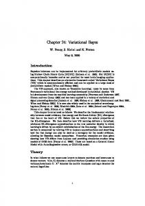
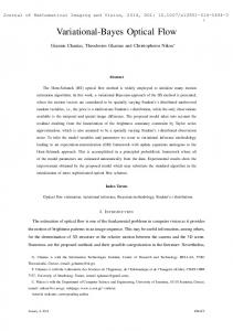
(75) where, again, we have dropped the constant term . The evidence and VB criteria are therefore identical, except for the divergences of and . However, as these do not scale with , we can ignore them. We also note that for large data sets, the distribution over is sufficiently peaked for the first expectation term not to make a significant difference, i.e., . We may also thus see the evidence approach as a limiting case of the VB framework. If we assume, a priori, that different model orders are equally likely, then the posterior probability distribution over model order is given by (29). This can also be applied to BIC/MDL. VI. RESULTS A. Synthetic Data: Gaussian Noise Model We generated multiple three second-blocks of 128 Hz data from AR(6) models with varying signal-to-noise ratios (SNRs). We also generated data from AR(25) models, again with varying SNRs. We generated ten data sets of each type (each with a different realization of the noise process) and applied the VB and BIC/MDL model order selection methods. Typical results are , SNR 2 and shown in Figs. 1 and 2, which are for , SNR 20, respectively.1 We have plotted the probability of each model order averaged over the ten runs (the averaging was done on the probabilities rather than the log probabilities in order to show a greater spread). For both the AR(6) and AR(25) data, model order selection is more difficult at lower SNR. For the AR(6) data, both methods essentially pick out the correct model order, with VB overestimating it on a small proportion of runs. For the AR(25) data, the BIC/MDL criterion significantly underestimates the model order. On longer blocks of data (e.g., 10 s), both methods were seen to converge to the same estimate of model order (as predicted by theory). B. Synthetic Data: Non-Gaussian Noise Model We generated 3 s of synthetic data from an AR(5) model with coefficients T

(72)

is the precision of the ML model. where The model order selection criterion for the evidence framework [see (66)] can be rewritten in terms of the KL-divergence . For between the weight posterior and the weight prior and the posterior the prior , it can be shown that

[see (68)], we can combine (73)

(74)

.

(76) and noise drawn from a two-component Gaussian mixture , and model with mixing coefficients , . We repeated the data generation variances as process ten times and used the negative free energy a model order selection criterion. The results in Figs. 3–5 show that the VB model order selection criterion selects both the correct AR order and the correct noise model order. For more on VB model order selection, including a comparison with the minimum description length (MDL) criterion, see [11]. We also calculated the error with which the AR coefficients . Over the ten were estimated using the measure 1The

SNR was altered by adjusting the noise variance.


2252


(a)

(a)

(b) Fig. 1. Model order selection for AR(6) data (SNR and (b) VB with 3-s blocks of data.

= 2) with (a) BIC/MDL

runs, the errors from the non-Gaussian AR model with two components were less than those from the Gaussian AR model by an average factor of six.

C. EEG Data: Gaussian Noise Model We applied AR models to short blocks of EEG data recorded while a subject was awake or in an anesthetized state. Fifty 1-s blocks were selected randomly from each 30-min recording, and BIC/MDL and VB model order selection criteria were compared. The results from VB in Fig. 6 show that in the waking state, and , and in the anesthetized there are modes at and . The results clearly state, the modes are at show a decrease in model order from the waking state to the anesthetized state; according to a t-test, this decrease is significant at the 0.0004 level. The results from BIC/MDL, however, showed no such discrimination. The difference of means was not significant; from a t-test, we get a significance level of 0.062.

(b) Fig. 2. Model order selection for AR(25) data (SNR and (b) VB with 3-s blocks of data.

= 20) with (a) BIC/MDL

D. EEG Data: Non-Gaussian Noise Model We applied the model to a short sample of EEG data shown in Fig. 7, the middle section of which is contaminated by an ), eye-movement artifact. For a Gaussian noise model ( , having the optimum AR model order was at . For and , the best models were also at (this is not always the case) with and . This shows that the non-Gaussian AR process with two noise components is the preferred model. This model took 25 iterations to converge. The final mixing coefficients in and , and the varithe noise model were and , ances (inverse precisions) were i.e., a low and high variance component. Fig. 7 shows which data points “belong” to which noise component. The first component corresponds to the majority of the data (78% of it), and the second component picks out the outliers that are mostly in the middle section. These points are then effectively downweighted in the corresponding weighted least squares regression. The outliers therefore have a minimal influence on the estimation of the



2253

(a)

(a)

(b)

(b)

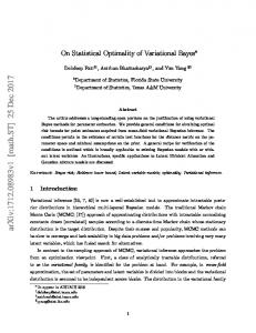
Fig. 3. AR model order selection (a) F (p; 2) versus corresponding probabilities P (p; 2) versus p.

p

AR coefficients; this can be seen from (54), where weight the samples accordingly.

and (b) the

and

Fig. 4. Noise model order selection (a) F (5; corresponding probabilities P (5; m) versus m.

m)

versus

m

and (b) the

in which we define the weight function (79)

E. How Good is the Variational Bound? From (23) we saw that the negative free-energy term formed a strict lower bound to the true posterior (the KL term is strictly non-negative). How tight this bound is will clearly affect the confidence we have in the variational approach. We consider here a simple experimental validation of the bound and present results on the non-Gaussian noise example in Section VI. Consider the marginal of (19), where once more, we drop, for notational convenience, dependence on

As noticed by others [22, ch. 4], this enables the variational apto be used as the proposal in an imporproximation tance sampling step. We do not cover the details of importance sampling as they may be found in standard texts (e.g., [23, ch. 5]). Suffice to say, the true posterior may be estimated via importance weights, which are evaluated as an expectation under the proposal, i.e., (78) may be written as

(77)

(80)

(78)

We applied this procedure to the non-Gaussian ) data analyzed in Section VI. A total AR( of 3s of data (384 samples) was generated from the true model, as before. The VB-AR algorithm was applied to this data, and then, using the variational inference densities as proposals, 1000 samples were evaluated using importance sampling to

We may write (77) as


2254


(a)

Fig. 5. Noise and AR model order selection. The bar plot shows against p; m.

P (p; m)

estimate the true model posterior.2 This was repeated over to 10 and with the number of all model orders from to 5. Fig. 8 shows Gaussians in the noise model from the relative increase in model evidence after the sampling grid. We note that the relative difprocedure over the ference between the “true” and approximate posteriors is of order one part in 10 at most (for these models). We note that the maximum model evidence appeared at the true model order in both cases. We note that, as expected from theory, the variational approximation is always a strict lower bound. It appears that the variational bound is very tight for low model orders but rises with increased numbers of model parameters, both in terms of the AR model order ( ) and, importantly, in terms of the number of mixture components in the noise model ( ). This is to be expected due to the factored nature of the variational approximation, which gets worse with increasing numbers of parameters. It is encouraging that the evidence “peaks” at the correct order in both cases, indicating that the variational free energy may offer a realistic model-selection criterion. More importantly, the use of the variational approximation as a proposal for importance sampling makes the latter very fast, and this approach is to be commended in cases where evaluation of the bound is crucial. VII. DISCUSSION We have proposed a non-Gaussian AR model for the modeling of stationary stochastic processes where the noise is modeled with a mixture of Gaussians. The main appli2As the dimensionality of the model increases, so does the tendency of the importance weights to be dominated by a small number of large weights. In the experiments reported here, this did not occur, although we note this tendency for high p models.

(b) Fig. 6. VB model order selection on EEG data from (a) awake subject and (b) anesthetized subject.

cation is as a model for stationary signals contaminated by non-Gaussian and/or nonstationary noise processes. The VB framework prevents overfitting and provides a model order selection criterion both for the AR order and the noise model order. In the experiments presented, we restricted the means in the noise mixture to be identically zero. The resulting model resembles weighted least squares and, hence, provides robust estimation of AR coefficients. Our model provides an alternative to cumulant methods for non-Gaussian AR modeling (see, e.g., [24] and [25]) for which model order estimation is problematic. We envisage that a main application of the model is to EEG data; in an EEG recording, up to 30% [26] of data blocks are corrupted by muscle, eye-movement, or other artifacts, and traditionally, these data blocks are discarded. As we have shown, however, the non-Gaussian AR model is able to downweight the contaminated section of each block, thus allowing more reliable AR (and consequently spectral) estimation. We also envisage using the non-Gaussian AR algorithm to model the sources in an independent component analysis model; this would extend the work in [10] by allowing for dynamic sources at the same



2255

Fig. 7. Top plot: Original EEG trace. Bottom plot: Log-probability that the data belongs to the first (low-variance) noise component log [calculated from (44)]. A high proportion of data in the middle section therefore clearly belongs to the second (high-variance) noise component. These points are downweighted in the estimation of the AR coefficients.

Fig. 8. Relative increase in evidence versus model order after importance sampling using the variational posterior as proposal.

time as using VB for model order estimation. It is noted that the model we use, in which the noise model has no dynamic struc-

ture, is equivalent to a 0th–order hidden Markov model (HMM) for the noise process with a number of hidden states equal to the number of components in the MoG. In the eye-movement artifact example, the high variance activity occurred sporadically, and the HMM(0) model is appropriate. It is arguable, however, that in some cases, where the high-variance noise occurs in temporally correlated bursts, that a higher order HMM is appropriate [a HMM(1), for example]. We have not considered this here, although it is an important area of future research. For Gaussian AR models, our experiments show that VB model order selection is superior to the BIC/MDL criterion. We have shown that for noninformative priors on the precision of the coefficients and the precision of the noise , the VB update rules are identical to those of the evidence framework. This is an extension of work by Mackay [21], who showed that for a linear regression model with known , the updates for are the same. This link therefore provides further justification for the updating rules used in the evidence framework (as the VB update rules probably increase a lower bound on the log-evidence, whereas no such convergence proof previously existed in the evidence framework). We have also shown that apart from minor differences that have no practical impact, the VB and evidence model order selection criteria are identical (again, under the assumption of noninformative priors on and ).


2256


B. Multivariate Normal Density

APPENDIX A DERIVATION OF VARIATIONAL LEARNING

The multivariate normal density is given by

We start by restating (27), which conjectures that the optimal form of the proposal ( ) distribution that maximizes the negative free energy (model evidence measure), with respect to parameter group , is (81)

T

(86)

The KL-divergence for normal densities and is

is the partition function (normalizing constant), and where where, as before, we define T

(82) This maximization is equivalent to stating that the negative and is maxKL-divergence between imized [this is strictly nonpositive and reaches its maximum when (81) holds]. The negative KL-divergence is given as

where

(87)

denotes the determinant of the matrix

.

C. Gamma Density The Gamma density is defined as (88)

(83) For Gamma densities , the KL-divergence is

Substituting from (82), we obtain

and

(89) where

is, as before, the digamma function [2].

D. Dirichlet Density The Dirichlet density is given by (84) where the last step follows from the factored representation of the proposal, i.e., (26). Note that this is (to within an additive constant) the contribution to the free energy of (24) of the parameter group . As the free energy is strictly non-negative, it is maximized by maximization of each contribution, e.g., maximization of ] (84). This is achieved when (81) holds, and hence, we obtain a simple methodology to obtain densities for each component of .

(90)

is the th element of , and where function [2]. For the -state Dirichlet density with and , the KL-divergence is

is the Gamma , ,

APPENDIX B DENSITIES AND DIVERGENCES For completeness, we include definitions of the normal, gamma, and Dirichlet densities and their entropies and KL-divergencies.

(91)

A. Univariate Normal Density For univariate normal densities , the KL-divergence is

and

(85)

ACKNOWLEDGMENT The authors would like to thank R. Daniel and P. Sykacek for interesting discussions and helpful comments and criticism of this work. The comments of the anonymous referees were most valuable in the final revision of this paper.



REFERENCES [1] C. M. Bishop, Neural Networks for Pattern Recognition. Oxford, U.K.: Oxford Univ. Press, 1995. [2] W. H. Press, S. A. Teukolsky, W. T. Vetterling, and B. V. P. Flannery, Numerical Recipes in C. Cambridge, U.K.: Cambridge Univ. Press, 1992. [3] G. Barnett, R. Kohn, and S. Sheather, “Bayesian estimation of an autoregressive model using Markov chain Monte Carlo,” J. Econometr., vol. 74, no. 2, pp. 237–254, 1996. [4] S. Godshill, “Bayesian enhancement of speech and audio signals which can be modeled as ARMA processes,” Statist. Rev., vol. 65, no. 1, pp. 1–21, 1996. [5] S. Godshill and P. Rayner, “Statistical reconstruction and analysis of autoregressive signals in impulsive noise,” IEEE Trans. Speech Audio Processing, vol. 6, pp. 352–372, July 1998. [6] P. Troughton and S. Godshill, “A reversible jump sampler for autoregressive time series, employing full conditionals to achieve efficient model space moves,” Dept. Eng., Univ. Cambridge, Cambridge, U.K., Tech. Rep. CUED/F-INFENG/TR.304, 1997. [7] S. Richardson and P. J. Green, “On Bayesian analysis of mixtures with an unknown number of components,” J. R. Statist. Soc. B, vol. 59, no. 4, pp. 731–758, 1997. [8] H. Lappalainen and J. W. Miskin, “Ensemble learning,” in Advances in Independent Components Analysis, M. Girolami, Ed. Boston, MA: Kluwer, 2000. [9] C. M. Bishop, “Variational principal components,” in Proc. Int. Conf. Artif. Neural Networks, 1999, pp. 509–514. [10] R. Choudrey, W. D. Penny, and S. J. Roberts, “An ensemble learning approach to independent component analysis,” in Proc. IEEE Int. Workshop Neural Networks Signal Process., Sydney, Australia, 2000. [11] W. D. Penny and S. J. Roberts, “Bayesian methods for autoregressive models,” in Proc. IEEE Int. Workshop Neural Networks Signal Process., Sydney, Australia, 2000. , “Variational Bayes for non-Gaussian autoregressive models,” in [12] Proc. IEEE Int. Workshop Neural Networks Signal Process., Sydney, Australia, 2000. [13] G. Kitagawa and W. Gersch, “A smoothness priors time-varying ar-coefficient modeling of nonstationary covariance time series,” IEEE Trans. Automat. Contr., vol. AC–30, pp. 45–56, 1985. [14] , “A smoothness priors long ar model method for spectral estimation,” IEEE Trans. Automat. Contr., vol. AC-30, pp. 57–65, 1985. [15] S. Weisberg, Applied Linear Regression. New York: Wiley, 1980. [16] J. J. K. O’Ruaniaidh and W. J. Fitzgerald, Numerical Bayesian Methods Applied to Signal Processing. New York: Springer, 1996. [17] T. M. Cover and J. A. Thomas, Elements of Information Theory. New York: Wiley, 1991. [18] H. Attias et al., “A variational Bayesian framework for graphical models,” in NIPS 12, T. Leen, et al., Eds. Cambridge, MA: MIT Press, 2000. [19] D. M. Chickering and D. Heckerman, “Efficient approximations for the marginal likelihood of Bayesian networks with hidden variables,” Microsoft Research, Tech. Rep. MSR-TR-96-08, 1996.

2257

[20] P. Sykacek, I. Rezek, and S. Roberts. (2000) Markov chain Monte Carlo methods for Bayesian sensor fusion. Dept. Eng. Sci., Univ. Oxford, Oxford, U.K., Tech. Rep. PARG-00-10. [Online]. Available: http://www.robots.ox.ac.uk/~parg/ [21] D. J. C. Mackay, “Ensemble learning and evidence maximization,” Tech. Rep., Cavendish Lab., Univ. Cambridge, Cambridge, U.K., 1995. [22] J. Miskin, “Ensemble learning for independent component analysis,” Ph.D. dissertation, Cavendish Lab., Univ. Cambridge, Cambridge, U.K., 2000. [23] J. M. Bernardo and A. F. M. Smith, Bayesian Theory. New York: Wiley, 1994. [24] S. Minfen, S. Lisha, and P. J. Beadle, “Parametric bispectral estimation of EEG signals in different functional states of brain,” in Advances in Medical Signal and Information Processing. London, U.K.: IEE, 2000, pp. 66–72. [25] C. L. Nikias, Higher-Order Spectra Analysis: A Nonlinear Signal Processing Framework. Englewood Cliffs, NJ: Prentice-Hall, 1993. [26] A. Gevins, M. E. Smith, and D. Yu, “High-resolution EEG mapping of cortical activation related to working memory: Effects of task difficulty, type of processing, and practice,” Cerebral Cortex, vol. 7, no. 4, pp. 374–385, 1997.

Stephen J. Roberts was born in London, U.K., in 1965. He received the Ph.D. degree in physics in 1991 from Oxford University, Oxford, U.K. He studied physics at Oxford from 1983 to 1986 and then worked for a few years in the Research Department of Oxford Instruments. From 1989 to 1991 he researched his Ph.D. and worked as a postdoctoral researcher until 1994, when he was appointed to the Faculty at Imperial College, University of London. In 1999, he joined Oxford. His main area of research lies in machine learning approaches to data analysis. He has particular interests in the application of machine learning methods to problems in mathematical biology. Current research focuses on Bayesian statistics, graphical models, independent component analysis, and information theory. He runs the Pattern Analysis and Machine Learning Research Group at Oxford. Dr. Roberts is a Fellow of Somerville College, Oxford.

Will D. Penny received the Ph.D. degree in electrical engineering from Imperial College, University of London, London, U.K., in 1993. He has since worked as a post-doctoral researcher at University College, London; Imperial College; and Oxford University, Oxford, U.K., and is now working as a brain-imaging statistician at University College. His research interests are in Bayesian statistics and data-driven machine learning and their application to biomedical data.
