Variational Shape Segmentation and Mesh ...

Abstract of thesis entitled

Variational Shape Segmentation and Mesh Generation Submitted by

YAN Dong Ming

for the degree of Doctor of Philosophy at The University of Hong Kong in March 2010 Surface reconstruction, shape segmentation and optimization are fundamental research problems in computer graphics and geometric modeling, which have numerous applications, such as reverse engineering, computer-aided design (CAD), computer-aided manufacturing (CAM), physical simulation, realtime rendering, biology and geography. The aim of surface reconstruction is to compute a compact shape representation from unorganized data points. Shape segmentation aims to decompose a complicated 3D model into meaningful sub-components for efficient processing. Shape optimization aims to compute another shape to approximate the original one, with better quality or other favorable properties required by specific applications. This thesis first studies the problems of variational shape segmentation, including quadric surface segmentation and segmentation of scanned botanical branching models. A novel approximate L2 distance metric from a point to a quadric surface is used to guide the segmentation of an input mesh into quadric patches. The segmentation is optimized via iteratively quadric surface fitting and clustering. The same segmentation framework is then used to segment scanned point data of tree models for reconstructing a compact surface representation. Isotropic surface remeshing and tetrahedral mesh generation are then studied. We propose robust and efficient algorithms for computing exact restricted Voronoi diagrams (RVD) on mesh surfaces and exact Voronoi diagrams of a 3D object. Together with a recently developed technique for fast computation of centroidal Voronoi tessellation (CVT), we present practical algorithms for both high quality surface remeshing and 3D tetrahedral mesh generation. [233 Words]

Variational Shape Segmentation and Mesh Generation by

YAN Dong Ming

A thesis submitted for the Degree of Doctor of Philosophy at The University of Hong Kong.

March 2010

Declaration I declare that this thesis represents my own work, except where due acknowledgement is made, and that it has not been previously included in a thesis, dissertation or report submitted to this University or to any other institution for a degree, diploma or other qualifications.

Signed:

Date:

iii

“Where There Is Matter, There Is Geometry”

Johannes Kepler (1571-1630)

Acknowledgements I am most indebted to my Ph.D. supervisor Prof. Wenping Wang for his continuous support and inspiration during the past years. The completion of this dissertation would not have been possible without his sound advice and guidance in each stage of my Ph.D. study. My sincere thanks to Prof. Bernard Mourrain and Dr. Julien Wintz in Project Galaad of INRIA Sophia Antipolis as well as Prof. Bruno Lévy in Project Alice of INRIA Nancy for their valuable assistance in getting results which contribute to this dissertation. I would like to express my gratitude to Prof. Hiromasa Suzuki for providing me the chance to visit RCAST of Tokyo University, and Prof. Niloy J. Mitra for inviting me to KAUST. I am particularly grateful to the members of our graphics lab for their companionship and sharing — Bin Chan, Loretta Yi-King Choi, Kelvin Kai-Wah Lee, Yang Liu, Dayue Zheng, Qi Su, Chen Liang, Xi Luo, Pengbo Bo, Lin Lu, Feng Sun, Grace Hui Zhang, Yufei Li, Ruotian Ling, Li Cao, Xiaohong Jia, Zhonggui Chen, Yuanfeng Zhou, Liping Zheng, Jung-Woo Chang, Zhengzheng Kuang, Zhan Yuan, Wenni Zheng and Yanshu Zhu. Together with the friends in Department of Computer Science — Lin Jiang and Veronica Yim, who have been staying by my side with their optimism and friendship, they all have given me countless pieces of precious memories and moments of enjoyment. The days in PGSA football team have been a most valuable memory in my HKU life. I hereby thank the guys Jian Li, Tao Peng, Liang Wang, Zhiguo Zhang, Zongxiang Xu and all the other teammates for sharing with me the fantastic recollections full of sweat and tears. Also my sincere appreciation for my old friends in Tsinghua University — Prof. Shimin Hu, Prof. Jean-Claude Paul, Hui Zhang, Huaiping Yang, Bin Wang, Yushen Liu, Yu Peng, Xiaodiao Chen, Weiming Dong, Liqiang Yue, Wenke Wang, Lei Yang, Piqiang Yu, Yijun Yang and Yongliang Yang for their cooperative and supportive friendship. I cannot thank my parents and sister enough for their love, sacrifice, patience and support which help me through all those difficult days in striving for a life of my desire. It is also to them that this dissertation is dedicated.

v

Contents Declaration

iii

Acknowledgements

v

List of Figures

1 Introduction 1.1 Background . . . . . 1.2 Variational geometry 1.3 Contributions . . . . 1.4 Outline . . . . . . .

ix

. . . . . . processing . . . . . . . . . . . .

. . . .

. . . .

. . . .

. . . .

. . . .

2 Variational Quadric Segmentation 2.1 Previous work . . . . . . . . . . . . . . . 2.2 Preliminaries . . . . . . . . . . . . . . . 2.2.1 Problem formulation . . . . . . . 2.2.2 Error metric for quadric proxies . 2.2.3 Quadric surface fitting . . . . . . 2.3 Variational quadric segmentation . . . . 2.3.1 Initialization . . . . . . . . . . . 2.3.2 Global optimization . . . . . . . 2.3.3 Post-processing . . . . . . . . . . 2.4 Experimental results . . . . . . . . . . . 2.5 Limitations and future work . . . . . . .

. . . .

. . . . . . . . . . .

. . . .

. . . . . . . . . . .

. . . .

. . . . . . . . . . .

. . . .

. . . . . . . . . . .

. . . .

. . . . . . . . . . .

. . . .

. . . . . . . . . . .

. . . .

. . . . . . . . . . .

. . . .

. . . . . . . . . . .

. . . .

. . . . . . . . . . .

. . . .

. . . . . . . . . . .

3 Variational Botanical Branching Model Reconstruction 3.1 Previous work . . . . . . . . . . . . . . . . . . . . . . . . . 3.2 Segmentation . . . . . . . . . . . . . . . . . . . . . . . . . 3.2.1 Preprocessing . . . . . . . . . . . . . . . . . . . . . 3.2.2 K-means clustering . . . . . . . . . . . . . . . . . . 3.2.3 Cylinder detection . . . . . . . . . . . . . . . . . . 3.2.4 Cluster subdivision . . . . . . . . . . . . . . . . . . 3.3 Branch reconstruction . . . . . . . . . . . . . . . . . . . . 3.3.1 Building adjacency graph . . . . . . . . . . . . . . 3.3.2 Skeleton extraction . . . . . . . . . . . . . . . . . . vii

. . . .

. . . . . . . . . . .

. . . . . . . . .

. . . .

. . . . . . . . . . .

. . . . . . . . .

. . . .

. . . . . . . . . . .

. . . . . . . . .

. . . .

. . . . . . . . . . .

. . . . . . . . .

. . . .

. . . . . . . . . . .

. . . . . . . . .

. . . .

. . . . . . . . . . .

. . . . . . . . .

. . . .

. . . . . . . . . . .

. . . . . . . . .

. . . .

. . . . . . . . . . .

. . . . . . . . .

. . . .

1 1 4 5 6

. . . . . . . . . . .

7 8 10 11 11 13 14 14 15 16 19 22

. . . . . . . . .

27 30 31 32 32 33 34 34 35 35

Contents

3.4

3.5 3.6

3.3.3 Branch identification Branch modeling . . . . . . 3.4.1 B-spline fitting . . . 3.4.2 B-spline lofting . . . Experimental results . . . . Limitations and future work

viii . . . . . .

. . . . . .

. . . . . .

. . . . . .

. . . . . .

. . . . . .

. . . . . .

. . . . . .

. . . . . .

. . . . . .

. . . . . .

. . . . . .

. . . . . .

4 Variational Isotropic Remeshing 4.1 Previous work . . . . . . . . . . . . . . . . . . . . . 4.2 Preliminaries . . . . . . . . . . . . . . . . . . . . . 4.2.1 Centroidal Voronoi tessellation . . . . . . . 4.2.2 Constrained CVT and restricted CVT . . . 4.2.3 Restricted Delaunay triangulation, validity 4.2.4 Algorithm overview . . . . . . . . . . . . . 4.3 RVD computation . . . . . . . . . . . . . . . . . . 4.3.1 Outline . . . . . . . . . . . . . . . . . . . . 4.3.2 Cell-triangle intersection . . . . . . . . . . . 4.3.3 Clipping by incident cells . . . . . . . . . . 4.3.4 Exact predicates . . . . . . . . . . . . . . . 4.4 Isotropic remeshing . . . . . . . . . . . . . . . . . . 4.4.1 Initialization . . . . . . . . . . . . . . . . . 4.4.2 Optimization . . . . . . . . . . . . . . . . . 4.4.3 Feature preservation . . . . . . . . . . . . . 4.4.4 Final mesh extraction . . . . . . . . . . . . 4.5 Experimental results . . . . . . . . . . . . . . . . . 4.6 Limitations and future work . . . . . . . . . . . . . 5 Variational Isotropic Tetrahedral Meshing 5.1 Previous work . . . . . . . . . . . . . . . . . 5.2 Preliminaries . . . . . . . . . . . . . . . . . 5.2.1 Clipped Voronoi diagram . . . . . . 5.2.2 Centroidal Voronoi tessellation . . . 5.3 Algorithm Overview . . . . . . . . . . . . . 5.4 Clipped Voronoi Diagram Computation . . 5.4.1 Voronoi diagram construction . . . . 5.4.2 Surface RVD computation . . . . . . 5.4.3 Clipped Voronoi cells construction . 5.5 Tetrahedral Mesh Generation . . . . . . . . 5.5.1 Initialization . . . . . . . . . . . . . 5.5.2 Optimization . . . . . . . . . . . . . 5.5.3 Final mesh extraction . . . . . . . . 5.6 Experimental results . . . . . . . . . . . . . 5.7 Limitations and future work . . . . . . . . .

. . . . . . . . . . . . . . .

. . . . . . . . . . . . . . .

. . . . . . . . . . . . . . .

. . . . . . . . . . . . . . .

. . . . . .

. . . . . . . . . . . . . . . . . .

. . . . . . . . . . . . . . .

. . . . . .

. . . . . . . . . . . . . . . . . .

. . . . . . . . . . . . . . .

. . . . . .

. . . . . . . . . . . . . . . . . .

. . . . . . . . . . . . . . .

. . . . . .

. . . . . . . . . . . . . . . . . .

. . . . . . . . . . . . . . .

. . . . . .

. . . . . . . . . . . . . . . . . .

. . . . . . . . . . . . . . .

. . . . . .

. . . . . . . . . . . . . . . . . .

. . . . . . . . . . . . . . .

. . . . . .

. . . . . . . . . . . . . . . . . .

. . . . . . . . . . . . . . .

. . . . . .

. . . . . . . . . . . . . . . . . .

. . . . . . . . . . . . . . .

. . . . . .

. . . . . . . . . . . . . . . . . .

. . . . . . . . . . . . . . .

. . . . . .

. . . . . . . . . . . . . . . . . .

. . . . . . . . . . . . . . .

. . . . . .

. . . . . . . . . . . . . . . . . .

. . . . . . . . . . . . . . .

. . . . . .

. . . . . . . . . . . . . . . . . .

. . . . . . . . . . . . . . .

. . . . . .

36 37 38 38 39 44

. . . . . . . . . . . . . . . . . .

45 48 49 49 50 51 53 53 54 54 56 56 58 58 58 59 60 62 73

. . . . . . . . . . . . . . .

75 77 77 77 78 79 80 80 80 81 82 83 84 85 85 88

6 Conclusion

91

Bibliography

95

List of Figures 1.1

1.2

2.1

2.2 2.3 2.4

2.5 2.6

2.7

2.8

2.9

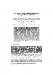
Various “meaningful” criteria for mesh segmentation: Buddha [133]; Feline [80]; Mask [41]; Venus (right) [142]; Dino [82]; Venus (left) [167]; Dragon [96] and Isis [64]. . . . . . . . . . . . . . . . . . . . . . . . . . . . . (a) Remeshing result of the Rockerarm model using the algorithm described in Chapter 4. (b) Tetrahedral meshing result of Joint model using the algorithm presented in Chapter 5. . . . . . . . . . . . . . . . . . . . . Segmentation (bottom row) and fitting (top row) results of Chess piece (12k triangles). Different colors of segmentation mean different proxies. (a)&(b) 300 planar proxies [41]; (c)&(d) 12 hybrid proxies [167]: 1 plane, 1 cylinder and 10 spheres; (e)&(f) 18 hybrid proxies [167]: 1 planes and 17 spheres; (g)&(h) 12 quadric proxies by our method: 2 planes, 2 spheres, 4 ellipsoids, and 4 hyperboloids of one sheet; (i) colors for different types of quadric surfaces. . . . . . . . . . . . . . . . . . . . . . . . . . . . . . Flowchart of our variational framework. . . . . . . . . . . . . . . . . . . Left: the red region is fitted by a degenerate quadric consisting of two intersecting planes; right: close-up view. . . . . . . . . . . . . . . . . . . Intermediate results of our method. New proxies are inserted progressively and the final projected result of this model is shown in Figure 2.1(d). (a) Result when the proxy number is 5; (b) result when the proxy number is 9; (c) Lloyd iteration finishes when proxy number is 12; (d) the boundaries in (c) are smoothed. . . . . . . . . . . . . . . . . . . . . . . Boundary smoothing. (a) Segmentation before boundary smoothing; (b) smoothed boundary. . . . . . . . . . . . . . . . . . . . . . . . . . . . . . Fandisk (13k triangles): two views of observation. (a)&(e) The input model; (b)&(f) partitioned by 22 quadric proxies; (c)&(g) result after boundary smoothing (λ = 1.0); (d)&(h) result after vertices projection. Tesa (22k triangles): (a) the input model; (b) partitioned by 12 quadric proxies; (c) boundary smoothing result (λ = 1.0); (d) vertices projection result. . . . . . . . . . . . . . . . . . . . . . . . . . . . . . . . . . . . . . CSG model (21k triangles): (a) the input model; (b) partitioned by 10 quadric proxies; (c) boundary smoothing result (λ = 1.0); (d) vertices projection result. . . . . . . . . . . . . . . . . . . . . . . . . . . . . . . Results of free-form objects. From left to right, the four figures on each row are the input models, final partitioned results, results after boundary smoothing, and results after vertices projection. (a)-(d) Homer (40k triangles): approximated by 61 quadric proxies (λ = 6.92); (e)-(h) Bunny (40k triangles): approximated by 28 quadric proxies (λ = 5.49); (i)-(l) Mask (62k triangles): approximated by 6 quadric proxies (λ = 4.06); (m)-(p) Bone (30k triangles): approximated by 5 quadric proxies (λ = 6.2). . . ix

3

4

. 9 . 14 . 15

. 16 . 17

. 20

. 20

. 20

. 21

List of Figures

x

2.10 Comparison with previous methods. (a)-(c): Findisk model approximated by 80 planar proxies [41], 24 hybrid proxies [167] and 22 quadric proxies by our method; (d)-(f): color coding of local errors. The RMS Hausdorff errors are 4.2 × 10−2 , 3.9 × 10−2 and 2.1 × 10−2 , respectively; (g)-(i): Tesa model approximated by 100 planar proxies [41], 14 hybrid proxies [167] and 12 quadric proxies by our method; (j)-(l): color coding of the local errors. The RMS Hausdorff errors are 3.4×10−2 , 4.8×10−2 and 4.0×10−3 , respectively. . . . . . . . . . . . . . . . . . . . . . . . . . . . . . . . . . . 23 2.11 Comparisons with Attene’s method [14]: top row: segmentation results of (a) Fandisk (23 regions), (b) Mug (10 regions) and (c) Cover (3 regions) models by [14] with 23 regions, respectively; bottom row: segmentation results of the same models by our method with the same number of regions. 24 2.12 Comparison with the method presented in [67]. (a) A scanned mechanical model with 40k faces; (b) segmentation result of [67] and (c) segmentation result of our method. . . . . . . . . . . . . . . . . . . . . . . . . . . . . . . 24 3.1

Tree model reconstruction pipeline. (a) Scanned data of an apple tree; (b) segmentation result, different color means different clusters; (c) branch identification result. The color of each branch is the same as its starting cluster; (d) final B-spline surface representation of tree branches. . . . . . 3.2 Intermediate results of the hybrid segmentation algorithm. Top row: segmentation results. From left to right, the numbers of clusters are 19, 60, 96, 214, respectively. Bottom row: bounding cylinders of the corresponding clusters. The green cylinders are fixed and those blue ones are unfixed. . . . . . . . . . . . . . . . . . . . . . . . . . . . . . . . . . . . . . 3.3 Skeleton generation. The background is the clustering result and the dash line means the branch connected to the root. Left: graph generated by connecting centers of neighboring cluster, which includes a loop in branching region (the triangle formed by three neighboring clusters). Right: skeleton generated by converting this graph into a tree. All the edges that do not belong to the shortest paths to the root cluster are removed. . . . . . . . . . . . . . . . . . . . . . . . . . . . . . . . . . . . . . 3.4 Definition of junction points. Upper left: the green spheres represent the center of each cluster, and the red spheres represent the internal junction points. Lower left: junction point of leaf node. Right: Skeleton generated by our method using junction points. . . . . . . . . . . . . . . . . . . . . 3.5 Illustration of lofting operation. . . . . . . . . . . . . . . . . . . . . . . . . 3.6 Reconstruction result of Melgueil. (a) Input point set; (b) segmentation result; (c) branch detection result; (d) skeleton and (e) lofting result. . . . 3.7 Reconstruction result of Walnut. (a) Input point set; (b) segmentation result; (c) branch detection result; (d) skeleton and (e) lofting result. . . . 3.8 Reconstruction result of Hetre. (a) Input point set; (b) segmentation result; (c) branch detection result; (d) skeleton and (e) lofting result. . . . 3.9 Comparison of skeleton results. The background is the clustered point data overlayed with the skeleton. (a) Skeleton generated by [168] with 357 clusters; (b) skeleton of our method with 356 clusters. Our method produces a better clustering and produces geometric details more faithfully. 3.10 (a) A scanned tree with two branches touch with each other; (b) zoom-in view. . . . . . . . . . . . . . . . . . . . . . . . . . . . . . . . . . . . . . .

28

32

35

36 39 41 42 43

44 44

List of Figures 4.1

4.2 4.3

4.4 4.5 4.6

4.7

4.8

4.9

4.10

4.11 4.12

4.13

Voronoi diagram computation and isotropic remeshing of the Kitten model (274k faces, 10k seeds). (a) Input mesh; (b) initial Voronoi diagram; (c) optimized result (RCVT); (d) remeshing result. . . . . . . . . . . . . . Centroidal Voronoi tessellation in a circle with constant density. (a) initial seeds; (b) after 5 Lloyd iterations and (c) CVT. . . . . . . . . . . . . . . RVD computation. (a) RVD of 200 seeds on a torus; (b) a zoom-in view of a restricted Voronoi cell; (c) a triangle of the input mesh (yellow) is shared by 3 incident Voronoi cells. . . . . . . . . . . . . . . . . . . . . . Constrained centroidal Voronoi tessellation and remeshing on a sphere. Illustration of restricted Delaunay triangulation in 2D. . . . . . . . . . . Intersection of a Voronoi cell and a triangle. (a) The triangle tj (blue) and the bounding planes of the Voronoi cell (black); (b) result after clipped by P0 ; (c) result after clipped by P1 to P5 ; (d) final result after clipped by P6 . The blue edges are part of the original edges of tj . The red edges are created by plane-polygon intersection. . . . . . . . . . . . . . . . . Clipping a triangle tj by its three incident Voronoi cells. (a) The dashed triangle is a Delaunay triangle formed by three seeds and the blue triangle tj is an input triangle; (b) clipping tj against x1 ’s Voronoi cell Ω1 , vertex v is the intersection between [q1 , q2 ] and bisector [x1 , x3 ]; (c), (d) propagation to Ω2 and Ω3 . . . . . . . . . . . . . . . . . . . . . . . . . . Remeshing with features. (a) RVD of the Mask model (3k faces, 1.5k vertices). The input mesh is in green and boundary curves in black. Here we use the vertices of input mesh as initial seeds (red); (b) Voronoi diagrams after 30 L-BFGS iterations, yielding a better distribution of seeds. The seeds of the boundary cells are snapped to the boundary to become feature seeds; (c) Voronoi diagram after 49 L-BFGS iterations, using the feature seeds provided in (b); (d) final remeshing result. . . . . Interleaving topology control / global optimization with density function ρ = 1. New vertices are progressively inserted to the regions where the Topological Ball Property are not satisfied. (a) Initial sampling with 4 vertices; (b) and (c) examples of non-manifold edges; (d) example of nonmanifold facets and (e) final result with validated topology. . . . . . . . RVD on the Bunny model (5k faces). The initial seeds are randomly distributed on the input mesh. From left to right are the Voronoi diagrams with different numbers of seeds: (a) 1k; (b) 10k; (c) 100k and (d) 500k. (e) The timing curve of seeds against processing time, with the number of seeds from 10 to 1M. The red curve is the time of Delaunay triangulation, the blue curve is the time of RVD computation and the green one is the time of kd-tree construction. . . . . . . . . . . . . . . . . . . . . . . . . . Remeshed David head, density ρ = 1/lf s2 . . . . . . . . . . . . . . . . . RVD (top row) and remeshing (bottom row) results of the Buddha model (300k faces and 50k seeds). The density functions are ρ = 1, ρ = |κmax | and ρ = |κmax |2 , respectively, from left to right. It takes 53 iterations and 400 seconds for the example in the middle. . . . . . . . . . . . . . . . . . Uniform CVT and remeshing results of models with shape features. Top: Fandisk model (13k faces, 3k seeds). It takes 100 iterations and 40 seconds; Bottom: Joint model (446 faces, 3k seeds), it takes 119 iterations and 49 seconds. From left to right are input meshes, results of RVD and RDT, respectively. . . . . . . . . . . . . . . . . . . . . . . . . . . . . . .

xi

. 46 . 49

. 50 . 51 . 52

. 55

. 57

. 60

. 61

. 63 . 64

. 67

. 68

List of Figures

xii

4.14 RVD and remeshing results of the Mask model with ρ = 1/lf s2 . (a) Input mesh; (b) optimized RVD without feature constrains; (c) final RVD result with feature constrains and (d) final RDT result. . . . . . . . . . . . . . . 4.15 Uniform remeshing of Dancer models. Top row: 13.7k faces, 10k seeds, 51 iterations in 56.7s. Bottom row: 13.9k faces, 10k seeds, 49 iterations in 50.3s. From left to right are input models, RVDs and RDTs, respectively. 4.16 Comparison of remeshing result. (a) Input model; (b) [157]; (c) [146]; (d) [21]; (e) [153]; (f) ours (48 iterations using 132 seconds). The quality comparison of these methods is given in Table 4.2. . . . . . . . . . . . . . 4.17 Comparison of uniform remeshing results. (a) [157]; (b) [146]; (c) ours. The quality comparison is listed in Table 4.2. . . . . . . . . . . . . . . . . 4.18 Uniform remeshing results of the noisy Balljoint (68.5k faces, 10k seeds). (a) Input mesh; (b) remeshing result of [157]; and (c) our result (259 iterations using 386 seconds). The quality comparison is given in Table 4.2. . . . . . . . . . . . . . . . . . . . . . . . . . . . . . . . . . . . . . . . 4.19 Comparison with DELPSC [36]. (a) Input model (20,886 vertices and 41,728 facets); (b) result of DELPSC [36], with required minimal angle as 30o , DELPSC produces 7,588 seeds and θmin = 2.79o ; (c) our result, with the same number of vertices and ρ = 1/lf s2 . We obtain θmin = 26o . The quality comparison is given in Table 4.2. Bottom row is the zoom-in view of homer hand. (d) Input mesh; (e) result of DELPSC [36]; (f) our result. . . . . . . . . . . . . . . . . . . . . . . . . . . . . . . . . . . . . . . 4.20 Comparison with [20]. The meshing quality is listed in Table 4.2. (a) Input Sphere model (163 vertices and 320 facets); (b) remeshing result of [20], with parameters θmin = 30o , size = 0.01 × diag, error = 1e−3 × diag; (c) our result with same number of vertices as (b). . . . . . . . . . . . . . 4.21 Topology control on Elephant model with ρ = 1/lf s2 . . . . . . . . . . . . 4.22 Topology control for Vase-Lion model, which has many details. Number of seeds is 10k and density ρ = 1/lf s2 . (a) Density function; (b) RCVT and (c) RDT. . . . . . . . . . . . . . . . . . . . . . . . . . . . . . . . . . . 4.23 An unsatisfactory remeshing result (5k seeds) of the Rabbit model. (a) Input noisy mesh; (b) RCVT and (c) remeshing result. . . . . . . . . . . 4.24 Uniform remeshing of a non-manifold mesh. (a) Input mesh with a nonmanifold edge; (b) result of RVD and (c) result of RDT. . . . . . . . . . 4.25 Uniform remeshing of a non-manifold mesh. (a) Input mesh with a nonmanifold facet; (b) result of RVD and (c) result of RDT. . . . . . . . . . 5.1

5.2 5.3

5.4

Clipped Voronoi diagram on 2D convex (a) and non-convex (b) domains. Yellow cells are boundary Voronoi cells. The number of seeds is 200 for each example. . . . . . . . . . . . . . . . . . . . . . . . . . . . . . . . . Illustration of propagation process. . . . . . . . . . . . . . . . . . . . . . Illustration of the proposed tetrahedral meshing algorithm. The blue wire frame is the boundary of input mesh. (a) Clipped Voronoi diagarm of initial sites; (b) result of unconstrained CVT with ρ = 1; (c) result of constrained optimization. Notice that boundary seeds are constrained on the surface S; (d) final uniform tetrahedral meshing result. . . . . . . . Timing curve of surface RVD computation against the number of seeds on Bunny model. . . . . . . . . . . . . . . . . . . . . . . . . . . . . . . .

68

69

70 70

70

71

71 72

72 73 74 74

. 78 . 81

. 83 . 86

List of Figures Result of volume VD computation. (a) Input Bone model (3, 368 tets and 1k boundary triangles); (b) VD of 100 seeds; (c) 1k seeds; (d) 10k seeds; (e) timing curve of VD computation against number of seeds. . . . . . . 5.6 Results of clipped Voronoi diagram computation. Brown cells are boundary cells and white cells are inner cells . . . . . . . . . . . . . . . . . . . 5.7 Uniform meshing of Torus model (20,837 input tets and 1k seeds). . . . 5.8 Adaptive meshing of Fertility model (22,139 input tets, 12k seeds). . . . 5.9 Uniform meshing result of Fandisk model (43.7k input tets, 5k seeds). . 5.10 Uniform meshing result of Joint model (35.2k input tets, 5k seeds). . .

xiii

5.5

. 87 . . . . .

88 89 89 90 90

Dedicated to my family

xv

Chapter 1

Introduction Digital 3D models are among the most popular and important media representations. Their applications include Computer-Aided Design (CAD), Computer-Aided Manufacturing (CAM), movie industry, scientific visualization, architecture design, physical simulation and so on. Regarding their ubiquitous presence in the digital world, the acquisition, modeling and processing of 3D digital models has attracted much attention during the last several decades.

1.1

Background

Early data acquisition techniques were mostly based on user manipulations, which usually require hours or even days to create a model with moderate complexity. And it was virtually impossible to digitalize complicated models of either large size or high precision. This situation has changed owing to the popularization of 3D laser scanners starting from the end of last century. In the Digital Michelangelo Project [92] launched in 1997, the group led by Prof. Marc Levoy from Stanford University obtained a highly precise 3D model of Michelangelo’s 5-meter statue in five years. Almost simultaneously, the Digital Forma Urbis Romae Project [93], another project by the same group, assembled 3D models for all 1, 186 fragments of the Forma Urbis Romae. Both projects provided high-precision and large-size scanned models which challenged computer graphics in a substantial way. More recently, the rapid improvements of scanning devices have enabled the digitalization of even more complex objects, such as real trees in the world [168]. Nowadays, digital geometric models are easy to obtain with 3D data acquisition devices, such as CT/MRI devices and 3D digital scanners. Not only precise models of ordinary size, but also huge and complex models of high quality can be acquired efficiently. 1

Chapter 1. Introduction

2

Polygonal and triangular meshes, as well as point based surfaces are important and popular shape representations of complex 3D models [26, 27, 84, 117, 176]. Raw data from 3D digital scanners, MRI or computer vision algorithms are often noisy and may contain many degenerate triangles. High level concise and faithful geometric representations of raw data are always desirable for geometry processing or rendering in various applications. In this thesis, we will study the fundamental problems of computing faithful high-level representations from raw data. Specifically, we are interested in the following problems: surface reconstruction, shape segmentation and mesh generation.

Surface reconstruction from point cloud data is one of the most fundamental problems in computer graphics and computational geometry. The input 3D models are often represented by a set of 3D unrecognized point data, probably with noise. Surface reconstruction aims to compute faithful surface representations directly from point clouds. Commonly used surface representations include piecewise linear, parametric and implicit surfaces. - Piecewise linear surfaces have the advantages of simple representation and easy processing, and can be used to represent objects with arbitrary topology. Hoppe et al.pioneered the piecewise linear surface reconstruction algorithms in 1990’s [73, 74]. Their approach has extensively been improved by many researchers in the following years [42]. - Parametric surfaces (e.g., subdivision surfaces or B-splines surfaces) have nice theoretical properties and simple computation form, hence are used in many industrial software tools. Meanwhile, different approaches have been proposed to fit smooth parametric surfaces to point cloud directly with guaranteed error control [35, 53, 97, 108]. - Implicit representation is another popular and powerful tool for surface representation, which can represent surfaces with arbitrary topology efficiently. Different types of implicit surfaces, such as radial basis function (RBF) [31], partition of unity (PU) [115] and point set surface (PSS) [2] have successfully been used in surface reconstruction from point data.

Shape segmentation

is another problem which gained a lot of focus in the past

decades. The scanned raw data are difficult to use directly for modeling, storage, visualization or transmission. The aim of shape segmentation is to decompose an input shape


3

Figure 1.1: Various “meaningful” criteria for mesh segmentation: Buddha [133]; Feline [80]; Mask [41]; Venus (right) [142]; Dino [82]; Venus (left) [167]; Dragon [96] and Isis [64].

into a set of components. Each component has a smaller size and simpler meaning, and therefore is easy to use for later processing. There are many “meaningful” metrics for different types of segmentation, among which the choice depends on users’ actual needs. Some examples of mesh segmentation are listed in Figure 1.1. Segmentation is always used as the preprocessing step in reverse engineering systems [17, 134, 135, 158– 160, 173]. It can also be used for parameterization (e.g. texture mapping) [94, 133], remeshing [5], mesh compression [81], shape modeling [63] (e.g. composition, matching) and so on. Readers are referred to Chapter 2 for more details about different types of mesh segmentation algorithms.

Mesh generation is an important research topic in both computer graphics and computational geometry community. In this thesis, we are interested in both surface remeshing and volume tetrahedral mesh generation. Surface remeshing aims to compute a new mesh to approximate a given input mesh surface with specified properties. Various remeshing algorithms have been proposed based on different requirements, such as regular or semi-regular remeshing [71, 72], isotropic or anisotropic remeshing [6, 7], VoronoiDelaunay based remeshing [19], quadrilateral or hexagonal remeshing [129, 164] and so on [3]. Tetrahedral mesh generation aims to fill a closed 3D volume with non-overlapping tetrahedra, such that the union of these tetrahedra is equal to the input volume. Similar to surface meshing, numerous approaches have been studied with respect to different meshing criteria [54]. Figure 1.2 shows two examples of isotropic surface remehsing and tetrahedral mesh generation, respectively.


(a)

4

(b)

Figure 1.2: (a) Remeshing result of the Rockerarm model using the algorithm described in Chapter 4. (b) Tetrahedral meshing result of Joint model using the algorithm presented in Chapter 5.

1.2

Variational geometry processing

The term “variational” in general suggests that the problem is solved using energy optimization. This approach has extensively been studied during recent years for solving different kinds of problems in geometry processing, such as surface remeshing [3], segmentation [41], reconstruction [11], vector field processing (e.g., vector field decomposition [152], vector field design [58] and visualization [48, 111]), surface deformation [24, 25, 98] and so on. A representative application of variational approaches is surface remeshing [5, 7]. Specifically, traditional parameterization based approach, which first segments an input mesh into charts and then parameterizes the charts onto 2D domains, is usually followed by a variational process using the Lloyd iteration [103], which optimizes a set of samples on each 2D domain and finally projects them back onto the surface to create the final remesh. An alternative method applies variational optimization directly to the input surface [157, 172], which avoids the parameterization steps. In addition, the variational approach was used by Gelas et al. for implicit surface meshing [66], and by some other researchers for isotropic tetrahedral mesh generation [8, 44, 153]. The variational framework can also be applied to shape segmentation. For example, Sander et al. proposed a chartification algorithm based on this framework to generate planar charts used in multi-chart geometry images creation. Cohen-Steiner et al. presented a variational shape approximation (VSA) algorithm, where the segmentation is driven by minimizing an energy function which measures the segmentation quality. This algorithm was later extended by replacing the energy function with other meaningful


5

metrics [80, 167, 171]. Apart from surface segmentation, the same framework was used as well in volume segmentation and bounding volume computation [85, 104, 142, 161].

1.3

Contributions

In this thesis, we present novel and efficient algorithms for computing high quality representations of 3D models from raw data, which is an essential step in many applications. The main contributions of this thesis include:

Quadric surface segmentation. A variational segmentation framework is proposed for extracting quadric components from input triangle meshes. Quadric proxies are introduced as a new type of surface primitives in addition to previously used planar proxies and simple quadric proxies, such as spheres and cylinders. A post-processing operator based on the graph-cut technique is developed to smooth segmentation boundaries. This algorithm works well for industry CAD models, scanned mechanical parts and free-form objects. We believe that this approach could be used in industrial CAD software in the future. Botanical branching reconstruction. Based on a modified k-means clustering algorithm, a pipeline is developed to reconstruct branch models of trees from laser scanned point data. The kernel of our system is a variational point cloud segmentation algorithm. Cylindrical components are detected at the segmentation stage while the connectivity are preserved by a kd-tree structure. The segmented components are then joined together to form the skeleton of the tree and branching structures are detected with simple heuristics. To our knowledge, this is the first attempt to reconstruct a branching system from laser scanned data. Variational isotropic remeshing. One of the most important contributions of this work is a fast and exact algorithm for computing the restricted Voronoi diagram (RVD) on a mesh surface with a given set of seed points. It has been believed that there was no efficient way to solve this problem in the past, therefore many approximation RVD computation algorithms were proposed. Based on an intuitive observation, i.e., a triangle facet must have intersection with the 3D Voronoi cell whose corresponding seed is the nearest neighbor of at lease one of the points on the facet, a novel and efficient algorithm is developed to identify the incident Voronoi cells of a given triangle. Then the intersection of each triangle with its incident cells is computed by a simple plane-polygon clipping algorithm. The resulting RVD on a mesh surface is the union of the intersected polygons of each seed. Our algorithm can work directly on triangle soup since it processes one triangle each time, with


6

no need for connectivity information. This algorithm is embedded in a variational CVT based remeshing framework. Integrated with a newly developed optimization technique, and quality remeshing results were achieved compared with state-of-art approaches. Isotropic tetrahedral meshing. A new CVT-based isotropic tetrahedral meshing algorithm is proposed. The main contribution of this work is an exact and fast algorithm for computing the clipped Voronoi diagram of a given closed 3D object. This algorithm enables us to use the recently developed efficient L-BFGS framework to compute a CVT. The clipped Voronoi diagram computation algorithm is a direct extension to the surface RVD computation algorithm [172]: the intersections between each tetrahedron and its incident 3D Voronoi cells are computed. By the fact that a Voronoi cell totally inside the object is the same as the 3D Voronoi cell of the same seed, the algorithm is simplified by restricting the computation to boundary cells only. Furthermore, the surface RVD computation algorithm proposed in [172] is improved by replacing the kd-tree query by a more efficient neighbor propagation approach.

1.4

Outline

The remainder of this thesis is organized as follows: in Chapter 2, a variational quadric segmentation method is presented; this segmentation framework is further extended to process point data in Chapter 3. As an application, a pipeline is proposed to reconstruct botanical branching structures of scanned trees. A practical isotropic remeshing system is introduced in Chapter 4. The heart of this system is a fast and exact algorithm for restricted Voronoi diagram computation on mesh surfaces. The RVD computation algorithm introduced in Chapter 4 is then extended to process a tetrahedral mesh in Chapter 5, and a new isotropic tetrahedral meshing algorithm is proposed. The summary and the conclusions are presented in Chapter 6.

Chapter 2

Variational Quadric Segmentation The quadric surfaces are flexible in both representation and processing, have powerful approximation ability [162]. Recovering quadric surfaces from raw data is needed for many applications [119], such as CAD/CAM modeling, reverse engineering or collision detection [39]. Based on the Lloyd iteration [103] (see Section 2.2), we present a variational method for extracting general quadric surfaces from a 3D mesh surface. This work extends the previous variational methods that extract only planes [41] or special types of quadrics, i.e., spheres and circular cylinders [167]. Instead of using the exact L2 error metric, we use a new approximate L2 error metric to make our method more efficient for computing with general quadrics. Furthermore, a novel method based on graph cut is proposed to smooth irregular boundary curves between segmented regions, which greatly improves the final results.

Contributions There are two contributions in this chapter. Firstly, motivated by the wide application and superior approximation power of quadrics e.g., nice geometric properties, easy computation), within the same clustering framework [41, 167], we further extend the surface types of proxies to include general quadric surfaces, or quadrics for short, plus planes. We show how the Euclidean distance from a triangle to a quadric can be computed in an approximate but efficient manner, while delivering robust segmentation results. Secondly, we propose a new method for smoothing irregular boundary curves between adjacent segmented regions through energy minimization using a graph cut approach.

7

Chapter 2. Variational Quadric Segmentation

8

This step produces more regular boundary curves, resulting in significantly improved segmentation results as compared with previous results (e.g., [167]).

Outline The remainder of this chapter is organized as follows. The related work to our approach is discussed in Section 2.1. Then we introduce the preliminaries of our work in Section 2.2 and present the quadric mesh segmentation framework in Section 2.3. Experimental results are demonstrated in Section 2.4 and we discuss the limitation of current work and give directions for the further research in Section 2.5.

2.1

Previous work

There are two areas of research that are closely related to our work: shape approximation and mesh segmentation. As described in Chapter 1, the main purpose of shape approximation is to compute a simple and compact surface representation of a complex geometric shape, based on different surface types or different computational approaches. We will mainly review those methods that employ the clustering approach.

Shape approximation.

Cohen-Steiner et al. [41] propose a shape approximation al-

gorithm based on the clustering approach to optimally approximate a mesh surface by a specified number of planar faces. This optimization problem is solved as a discrete partition problem using the Lloyd algorithm [103], which is commonly used for solving the k-mean problem in data clustering. There are two iterative steps in this method: mesh partition and fitting a plane surface, called a proxy, to each partitioned region. This method proves effective especially for extracting features and planar regions, but tends to produce an overly large number of planar proxies for a good approximation of a free-form surface. Because of its optimization nature, the method is often referred to as a variational method. Wu and Kobbelt [167] extend the work in [41] by introducing spheres, cylinders and rolling ball patches as additional basic proxy types, so that a complex shape can be approximated to the same accuracy by a much fewer number of proxies, leading to a more compact representation. However, these newly added surface types mentioned are still rather restrictive, even for CAD models and other man-made objects. For example, the middle part of the Chess piece in Figure 2.1 cannot be well approximated either by a circular cylinder or a collection of spherical or planar surface strips.


9

(i) Figure 2.1: Segmentation (bottom row) and fitting (top row) results of Chess piece (12k triangles). Different colors of segmentation mean different proxies. (a)&(b) 300 planar proxies [41]; (c)&(d) 12 hybrid proxies [167]: 1 plane, 1 cylinder and 10 spheres; (e)&(f) 18 hybrid proxies [167]: 1 planes and 17 spheres; (g)&(h) 12 quadric proxies by our method: 2 planes, 2 spheres, 4 ellipsoids, and 4 hyperboloids of one sheet; (i) colors for different types of quadric surfaces.

Simari et al. [142] use ellipsoids as the only type of proxies for approximating mesh surfaces, again using the Lloyd’s method with the error metric being a combination of Euclidean distance, angular distance and curvature distance. The segmentation boundaries are smoothed by a constrained relaxation of the boundary vertices. They also approximate the volume bounded by a mesh surface using a union of ellipsoids, where whole ellipsoids, rather than ellipsoidal surface patches, are used. Julius et al. [80] segment mesh surfaces into developable surface charts for texture mapping and pattern design. Open segmentation boundaries are straightened by a shortest path algorithm and interior segmentation boundaries are smoothed by a graph cut method similar to that described in [82]. Attene et al. [14] extend the hierarchical face clustering (HFC) approach [64] by introducing higher order fitting primitives. A binary cluster tree is created from bottom to top. At each iteration, every pair of adjacent clusters are fitted by a plane, a sphere and a cylinder. A pair of adjacent clusters with the minimal fitting error is merged into one cluster. The smoothing of segmentation boundaries is not considered. Implicit surfaces have long been used for shape approximation and segmentation. Based on region growing, Besl et al. [18] segment range image data by fitting implicit surfaces of variable orders. Fitzgibbon et al. [59] improve this work, also using region growing,


10

to fit general quadric surfaces and planes to the range images, and compute surface intersections to extract a B-rep from the segmented image. Since region growing and region merging approaches rely mainly on local consideration, such as curvature estimation or local fitting, the segmentation result can be poor when there is no obvious curvature discontinuity, e.g., when two quadric patches join with near G1 continuity. In this regard the iterative variational method has a distinct advantage that the local error in partition can be corrected by the fitting process, and the improved partition in turn provides a more reliable basis for better fitting (see Figure 2.11 and 2.12 for comparisons with region merging approaches).

Mesh segmentation.

Besides being used as a preparatory step for surface approx-

imation, mesh segmentation is also used to partition a surface model into meaningful parts for various other purposes. There are mainly two different types of mesh segmentations algorithms, part based [77, 82, 83, 87, 88, 90, 91, 100, 106, 174] and patch based [14, 38, 109, 126, 133, 160, 167, 169, 170]. A most recent approach by Chen et al. [34] describes a benchmark for evaluation of 3D mesh segmentation algorithms. A detailed discussion of mesh segmentation methods is out of the scope of this chapter. We refer the reader to the survey in [15, 136, 137] and references therein. Two recent methods for mesh segmentation are worth mentioning. Katz et al. [82] use fuzzy clustering and graph cut to segment a mesh. The mesh is first clustered by the geodesic distance. A fuzzy region is created between every two adjacent components. Finally the fuzzy region is segmented by a graph cut method to yield a smooth boundary. Lavoué et al. [89] present a mesh segmentation algorithm based on curvature tensor analysis. The mesh is first decomposed into several patches, each patch with nearly constant curvature. Then the segmentation boundary is rectified based on the curvature tensor directions. Smoothing boundaries between adjacent segmented regions is usually considered as a post-processing step after mesh segmentation [80, 82, 83, 89]. We propose a new graph cut based strategy to smooth the segmentation boundary, which considers both the approximation error and the smoothness of the boundary between neighbor regions, and delivers better results in smooth regions of a surface (e.g., see Figure 2.4(d)).

2.2

Preliminaries

In this section we describe the problem formulation of the variational shape approximation and introduce a new error function for measuring the distance between a mesh


11

surface and a quadric surface.

2.2.1

Problem formulation

Let M denote an input mesh surface, and T denote the set of triangles of M. Suppose that M is partitioned into n non-overlapping regions, denoted by R = {Ri }ni=1 , each S i region Ri contains a set of triangles Ti = {tik }nk=1 such that ni=1 Ti = T . Each region is approximated by a quadric proxy (including the plane as a special case). A quadric proxy, denoted by Pi , is represented by the coefficients of its associated quadratic form. A seed face, denoted by si , is a triangle face in Ti that has the smallest error to the quadric proxy Pi . In a variational framework, the optimal partition R = {Ri }ni=1 is found by minimizing the following objective function [41]: E(R, P) =

n X

E(Ri , Pi ),

(2.1)

i=1

where E(Ri , Pi ) is the error between the partitioned region Ri and its approximating proxy Pi . The above objective function (Eqn. 2.1) can be minimized by Lloyd’s algorithm (invented in 1957 [102], published in 1982 [103]) through iterative partition and fitting. Lloyd iteration is a powerful tool originally devised for optimal signal quantization. It has successfully been used in data clustering, such as the k-means clustering algorithm [76]. Recently, Lloyd’s method has been customized for many applications in computer graphics and geometry modeling [4]. We will define the error terms used in our method in the following of this section (Section 2.2.2 and 2.2.3) and then present our segmentation framework in Section 2.3.

2.2.2

Error metric for quadric proxies

The objective function in the variational shape approximation framework is defined in terms of error terms. Both L2,1 and L2 metrics have been tested in [41, 167]. For planar proxies, it is possible to derive closed formulas of L2,1 and L2 error terms, and L2,1 proves to produce better results. Wu and Kobbelt [167] use an approximate L2 error term to measure the distance from a triangular face to a hybrid proxy, which is a sphere, a circular cylinder or a rolling ball blending surface, expressed in terms of the exact L2 distances from the three vertices of the triangle to the proxy.


12

While it is easy to compute the Euclidean distance from a point to a sphere or a circular cylinder, it is not desirable to use the same error term as in [167] when extending proxy types to general quadric surface, because computing the exact distance from a point to a quadric involves solving for the roots of a degree six univariate polynomial. This is a very time consuming task, because the distance computation needs to be performed for many vertices/triangles of a large mesh in many iterations – according to our test on an implementation based on computation of the exact Euclidean distance, each iteration takes about 20 seconds for a mesh of 10K vertices on a PC with a Xeon(TM) 2.66 GHz CPU. This would render our method too inefficient. Assume that the function f (x, y, z) is given as: f (x, y, z) = C0 + C1 x + C2 y + C3 z + C4 x2 + C5 xy + C6 xz + C7 y 2 + C8 yz + C9 z 2 , (2.2) and f (x, y, z) = 0 is a quadric surface, denoted by Z(f ). We have also tested both algebraic distance δ0 = |f | and first-order approximation δ1 =

|f | k∇f k

in our algorithm.

But they turned out not to work well due to relatively large approximation errors. Balancing efficiency and accuracy, we choose to use Taubin’s second order approximation of the Euclidean distance δ2 (p, Z(f )) from the point p to the surface Z(f ) [149]. This approximate distance δ2 (p, Z(f )) has the favorable property that it is bounded between 0 and the exact L2 distance from p to Z(f ). For quadric surfaces, δ2 (p, Z(f )) is given by the only non-negative root of a quadratic polynomial g(t) = at2 + bt + c, where

a = − (C52 + C62 + C82 )/2 + C42 + C72 + C92

1/2

,

b = − (C1 + [2C4 , C5 , C6 ] · p )2 + (C2 + [C5 , 2C7 , C8 ] · p )2 + 1/2 (C3 + [C6 , C8 , 2C9 ] · p )2 , c = |f (p)|. Based on this approximate distance, the approximated L2 distance between a triangle tj and a quadric surface Pi is defined as: m

d(tj , Pi ) =

1 X δ2 (pk , Zi (f ))2 · |tj |, m

(2.3)

k=1

where {pk }m k=1 are uniformly sampled points on the triangle tj , and |tj |, the area of tj , serves as a weighting factor to account for triangles of different sizes. In implementation we set m = 4, i.e., use the vertices and the barycenter point of ti , and have obtained satisfactory results.


13

The approximated L2 distance between Ri and Pi is then defined as: E(Ri , Pi ) =

X

d(tj , Pi )/|Ri |,

(2.4)

tj ∈Ri

P

where |Ri | =

e 2 to denote this approximation |tj | is the area of region Ri . We use L

tj ∈Ri

to L2 distance. To have a uniform comparison, all mesh surfaces are scaled uniformly to fit in a rectangular box with their longest side being 1.

2.2.3

Quadric surface fitting

Given a region Ri , we need to fit a quadric surface to Ri in L2 metric. Two common ways of fitting implicit surfaces are the algebraic distance-based fitting and orthogonal distance-based fitting [1]; in general, the latter produces better fitting results than the former but is computationally much more costly. Since surface fitting is performed repeatedly in our present application, it is not necessary to take much time to compute the best fitting result in L2 metric in each single intermediate iteration. Hence, we use Taubin’s method [148] based on a first-order approximation of L2 metric for quadric surface fitting. Let f (x, y, z) = 0 be a quadric surface (see Eqn. 2.2). The squared distance from a point p to the implicit surface Z(f ) = {(x, y, z)|f (x, y, z) = 0, x, y, z ∈ R} is approximated f (p)2 . The original method proposed by Taubin is applied to a by δ1 (p, Z(f ))2 ≈ k∇f (p)k2 set of data points. Given a set of points {pi , i = 1, · · · , n}, the sum of approximated squared distance is, following [148] n 1 P f (pi )2 n X n 1 CT M C i=1 δ1 (pi , Z(f ))2 ≈ = , n 1 P n CT N C i=1 k∇f (pi )k2 n i=1

where M, N are coefficient matrices and C = [C0 , C1 , . . . , C9 ]T . For our application, we need to treat the data points as the continuum of surface points distributed uniformly over the mesh surface. Therefore, we adapt Taubin’s method by defining the sum of approximated squared distance as follows:

1 |Ri |

ni R 1 P 2 tk f (p) dp |R | CT Mt C i k=1 δ1 (p, Z(f ))2 dp ≈ = , ni R 1 P CT Nt C tk 2 dp k∇f (p)k |Ri | k=1 tk

ni Z X k=1

(2.5)


14

where Mt , Nt are coefficient matrices (see Appendix 2.5 for details). Hence, the fitting problem is reduced to computing the eigenvector of Mt − λNt associated with the minimum eigenvalue [148]. The detailed formula of the quadric fitting is given in Appendix 2.5. Although, due to efficiency consideration, only approximations to the L2 error metric (i.e., the true squared Euclidean distance) are used in our fitting and partitioning steps, we find that this treatment works robustly and efficiently in practice with the variational shape approximation framework.

2.3

Variational quadric segmentation

There are three steps in our quadric segmentation framework: initialization, global optimization and post-processing. Figure 2.2 shows the main flow of our algorithm. We will explain each of them in detail in the following.

Figure 2.2: Flowchart of our variational framework.

2.3.1

Initialization

In this step, we randomly choose n initial seed faces. Then each seed face determines a planar proxy which is the containing plane of the seed face. Then a distortion-minimizing flooding [41] is performed to give an initial partitioned mesh consisting of n regions R = {Ri }ni=1 .


15

Distortion-minimizing flooding. The aim of distortion-minimizing flooding is to partition the input mesh into a set of non-overlapping, connected regions {Ri }ni=1 . Given a set of seed triangles {si }ni=1 and their corresponding proxies {Pi }ni=1 , we first compute the distance between all the neighboring triangles of each seed triangle si and its corresponding proxy Pi . All the tested pairs (tj , Pi ) are inserted into a global priority queue ˜ with a priority equal to d(tj , Pi ) (Eqn. 2.3). In each step the triangle-proxy pair (t˜, P) with the smallest distance is popped out from the queue. If t˜ is already assigned to a region we continue the procedure without doing anything; otherwise t˜ is assigned to the region against which it is tested. Then we test all the unlabeled neighboring triangles of t˜ with the current proxy P˜ and push these new triangle-proxy pairs into the queue. This process is repeated until the queue is empty. Finally we shall get a new partition of the input mesh. The reader is referred to [41] for more details of this algorithm.

2.3.2

Global optimization

Once we have a new partition R of the surface mesh M, the two alternative steps of quadric surface fitting and region partitioning are performed iteratively to reduce the value of the objective function until convergency or a maximal number of iterations is reached (we choose 30 in all our experiments). Typically we choose the number of regions n = 1 at the beginning and the new proxies are inserted progressively. The algorithm terminates when an error threshold is met and the Lloyd iteration has converged. Proxies are inserted or merged to achieve the optimal approximation, as described below. Other proxy operations, such as proxy deletion or teleportation, have also been implemented, as in [41].

Proxy insertion.

When the Lloyd iteration has converged, we need to check the

validity of each quadric proxy. If the quadric surface degenerates to a pair of planes or is

Figure 2.3: Left: the red region is fitted by a degenerate quadric consisting of two intersecting planes; right: close-up view.


(a)

(b)

16

(c)

(d)

Figure 2.4: Intermediate results of our method. New proxies are inserted progressively and the final projected result of this model is shown in Figure 2.1(d). (a) Result when the proxy number is 5; (b) result when the proxy number is 9; (c) Lloyd iteration finishes when proxy number is 12; (d) the boundaries in (c) are smoothed.

a hyperboloid of two sheets and the projected data points are contained in both sheets, the proxy is considered as invalid, since it is not an appropriate representation. If such a case occurs, new proxies will be inserted in such a region. Figure 2.3 gives an example of a region fitted by one degenerate quadric consisting of two intersecting planes, which needs to be split into two separate planar proxies. If every proxy is valid but the fitting error is still larger than a pre-specified threshold, we use the farthest-point criterion to add a new proxy Pnew ; that is, we first find the region e 2 error belonging to this with maximal fitting error and a face which has the largest L region as the seed face snew . The new proxy Pnew is then set to be the plane containing the seed face snew . Then the Lloyd iteration is continued. Figure 2.4 illustrates some intermediate steps of our algorithm.

Proxy merging.

When the Lloyd iteration converges, we also check whether there

are redundant proxies by considering merging each pair of adjacent regions Ri and Rj . We use a quadric surface Pt to fit the union of Ri and Rj . Let Et be the fitting error. If |Et − (E(Ri , Pi ) + E(Rj , Pj ))| < (we set = 0.5 × max{E(Ri , Pi )}, as in [41]), and Pt i

is a valid proxy, then Ri and Rj are merged into one region. If there are several pairs which can be merged at the same time, the pair with the smallest fitting error is chosen to be merged first.

2.3.3

Post-processing

Several approaches are proposed to improve the segmentation quality in this section, including boundary smoothing, simple quadric types classification and proxy projection.


(a)

17

(b)

Figure 2.5: Boundary smoothing. (a) Segmentation before boundary smoothing; (b) smoothed boundary.

Boundary smoothing.

After the global optimization stage, the surface mesh M has

been partitioned into non-overlapping regions Ri , each been fitted by a quadric proxy e 2 errors Pi . Triangle faces next to region boundary curves always have nearly equal L (which are near the intersection curve of two adjacent quadrics), often leading to zigzag boundary curves. The graph cut method has already been used in [80, 82, 83] to segment mesh in the fuzzy region and boundary regularization, but only dihedral angle and edge length are used in their approach, so it works well mainly in regions with salient features or curvature discontinuity. We propose a new graph cut based strategy which is particularly effective for smoothing boundary curves in a smooth region of the mesh. Consider the dual graph of the original mesh, with each triangle face corresponding to a dual vertex. Given two neighboring regions R0 and R1 , the faces belonging to the neighbor of their common boundary are marked as belonging to the fuzzy region (Figure 2.5(a) illustrates the fuzzy region. The size of neighbor can be set by the user.). Let Vf denote the set of the dual vertices of the fuzzy region. Suppose that the faces in the fuzzy region are removed from R0 and R1 . Then the dual vertices of faces in the regions R0 and R1 that are adjacent to Vf are denoted as V0 and V1 , respectively. The goal of boundary smoothing is to label the vertices in Vf with 0 or 1 by minimizing a cost function E(X). This is similar to the binary labeling problem for edge detection widely used in image segmentation. The solution X is a binary vector X = [x0 , x1 , . . .], xi ∈ {0, 1}. If vi ∈ Vf is labeled with 0, i.e., set xi = 0, then its corresponding face is assigned to the region R0 ; otherwise, if xi = 1, the face is assigned to the region R1 . Let G = {V, E} be an undirected sub-graph of the dual graph of the mesh M, where V = Vf ∪ V0 ∪ V1 is the set of nodes. Here E is the set of undirected edges, with each dual edge e = (vi , vj ), (vi , vj ∈ V, i 6= j) corresponding to an edge shared by two adjacent faces in V. In Figure 2.5 the background is composed of two regions R0 and R1 . The


18

set V0 consists of the green triangles in R0 , the set V1 consists of the red triangles in R1 , and the set Vf consists of those triangles between V0 and V1 . Here V0 and V1 are hard constraints to R0 and R1 in the sense that the triangles in both sets will keep their labels; only the triangles in Vf may be re-labeled. The energy function E(X) is defined in a similar way to [95] used for image segmentation: E(X) = E1 (X) + λE2 (X) =

X vi ∈V

ˆ1 (xi ) + λ E

X

ˆ2 (xi , xj ). E

(vi ,vj )∈E

In order to keep the triangle faces in the fuzzy region from deviating too much from their quadric proxies and improve boundary smoothness, we consider both the distance from the boundary faces to their proxies and the edge length along the boundary. The region energy term E1 is determined by how the nodes vi in Vf are labeled. Let d0i = d(vi , P0 ) e 2 distance of vi to proxies P0 and P1 . Then we define and d1i = d(vi , P1 ) be the L

ˆ1 (xi = 0) = E

        

0,

vi ∈ V0

∞, vi ∈ V1 ; 0 di , vi ∈ Vf 0 di + d1i

ˆ1 (xi = 1) = E

        

∞,

vi ∈ V0

0, vi ∈ V1 1 di , vi ∈ Vf 0 di + d1i

ˆ2 is the cost of a dual edge connecting two adjacent face nodes {vi , vj }, and The term E defined by ˆ2 (xi , xj ) = E

length(i, j) |xi − xj |, length(i, j) + ave length

where length(i, j) is the length of the common edge shared by vi and vj , and ave length is the average edge length of the mesh M [82]. Clearly, E2 (X) becomes larger when the edge length of the cut boundary resulting from re-labeling is longer. The cost function E(X) is minimized using the max-flow/min-cut algorithm described in [30]. Figure 2.5(b) shows the result after running the max-flow algorithm. For different mesh models, two parameters in the above smoothing algorithm can be set by the user in order to obtain satisfactory results. For the CAD models with clear structure, such as the Fandisk and the Chess piece, the one ring neighborhood of the boundary usually suffices; and we use λ = 1.0 for this type of models in all the examples presented in this chapter. For the free-form objects like the Bunny, Homer, the two- or three-ring neighbor of the boundary works well in our experiments; and the value of λ is selected by the user in the interval [1, 10].

Quadric surface classification.

To simplify the final representation, we would like

to identify some commonly used types of special quadrics, such as spheres and circular


19

cylinders, which have occurred as approximating proxies. Given the coefficients of proxy Pi , we detect whether the quadric is nearly a cylinder or a sphere by analyzing the eigenvalues of the corresponding quadratic form [59]. After type identification, the region is fitted by a quadric of the special type that has been identified. Only circular cylinders and spheres are considered as special types in our current implementation.

Proxy projection.

As the final step of post-processing, the vertices of each region

Ri of the partitioned mesh M are projected onto the corresponding proxy Pi of Ri . The computation of foot points on a plane, sphere or cylinder is straightforward. If the quadric surface belongs to some other types, we compute the exact foot point by solving a degree six univariate equation [59]. For an interior vertex of a region Ri , its projected position is the foot point on the proxy of Ri ; if a mesh vertex is shared by two or more regions, the final position is the average of its foot points on all the proxies the vertex belongs to.

2.4

Experimental results

In this section we present some test examples to show the effectiveness of our method and to compare it with some previous methods that are also based on variational shape approximation. These examples are shown in Figures 2.6, 2.7, 2.8 and 2.9. The meaning of colors of the projected results is given in Figure 2.1(i). All the examples were run on a PC with a Xeon (TM) 2.66GHz CPU. We use TNT library1 to solve the eigenvalue problem in Section 2.2.3. Table 2.1 gives the running time and other statistics of all the examples. It can be seen that our method works well for CAD models or CSG objects with salient features (Figures 2.6, 2.7, 2.8), as well as for free-form geometry (Figure 2.9). Mesh Fandisk Tesa CSG Chess Bunny Homer Mask Bone

No. of faces 13K 22K 21K 24K 40K 40K 62K 30K

No. of proxies 22 12 10 12 28 61 6 5

Lloyd iteration (sec.) 11 18 16 15 103 148 203 14

Table 2.1: Timing Statistics.

1

http://math.nist.gov/tnt/

Post-processing (sec.) 0.017 0.042 0.031 0.100 0.352 0.393 0.115 0.067


(a)

(e)

20

(b)

(c)

(f)

(g)

(d)

(h)

Figure 2.6: Fandisk (13k triangles): two views of observation. (a)&(e) The input model; (b)&(f) partitioned by 22 quadric proxies; (c)&(g) result after boundary smoothing (λ = 1.0); (d)&(h) result after vertices projection.

(a)

(b)

(c)

(d)

Figure 2.7: Tesa (22k triangles): (a) the input model; (b) partitioned by 12 quadric proxies; (c) boundary smoothing result (λ = 1.0); (d) vertices projection result.

(a)

(b)

(c)

(d)

Figure 2.8: CSG model (21k triangles): (a) the input model; (b) partitioned by 10 quadric proxies; (c) boundary smoothing result (λ = 1.0); (d) vertices projection result.


21

(a)

(b)

(c)

(d)

(e)

(f)

(g)

(h)

(i)

(j)

(k)

(l)

(m)

(n)

(o)

(p)

Figure 2.9: Results of free-form objects. From left to right, the four figures on each row are the input models, final partitioned results, results after boundary smoothing, and results after vertices projection. (a)-(d) Homer (40k triangles): approximated by 61 quadric proxies (λ = 6.92); (e)-(h) Bunny (40k triangles): approximated by 28 quadric proxies (λ = 5.49); (i)-(l) Mask (62k triangles): approximated by 6 quadric proxies (λ = 4.06); (m)-(p) Bone (30k triangles): approximated by 5 quadric proxies (λ = 6.2).

Chapter 2. Variational Quadric Segmentation Comparison.

22

The RMS Hausdorff errors (divided by the length of bounding box

diagonal) by our method and the methods in [41] and [167] are presented in Figure 2.10. We use Metro tool [40] to measure the RMS Hausdorff errors between approximate and original models. It can be seen that the proposed method in this chapter gives a more compact or more accurate approximation. We also compare our approach with the region merging based method [14]. The algorithm proposed by Attene et al. [14] is very fast but the segmentation relies on the local information of the mesh. The result would be poor in both blending regions and regions of complex surfaces. Comparisons with [14] are given in Figure 2.11. Our method can obtain better results but with longer computation time. Figure 2.12 demonstrates that our method obtains better result when segmenting the models with blending regions compared to the region merging method presented in [67].

2.5

Limitations and future work

An unsatisfactory example. Our algorithm may behave poorly in some cases. One such example is shown in the right inset. The input model is a convex smoothed octahedra, the image on the left is the result of VSA [41] and that on the right is our result. Although our result has smaller fitting error, the appearance of segmentation looks poor since quadric surfaces are too flexible for this model.

Better initialization. Our algorithm can produce satisfactory segmentation results for various types of input meshes. However, the variational approaches [41, 80, 167, 171] suffer from the randomized initial seeds selection. Initial seeding is crucial to the convergence speed and segmentation quality. In the future, we would like to investigate new methods for efficient initial seeds selection, which will greatly help the subsequent optimization process.

More fitting types.

We focus on general quadric surfaces extraction in this work.

However, in industrial CAD/CAM applications, simple elements, such as spheres, cylinders, cones and torus are commonly used. We plan to enrich the basic fitting elements in our framework, which can make our framework suitable for more types of input.


23

(a)

(b)

(c)

(d)

(e)

(f)

(g)

(h)

(i)

(j)

(k)

(l)

Figure 2.10: Comparison with previous methods. (a)-(c): Findisk model approximated by 80 planar proxies [41], 24 hybrid proxies [167] and 22 quadric proxies by our method; (d)-(f): color coding of local errors. The RMS Hausdorff errors are 4.2 × 10−2 , 3.9 × 10−2 and 2.1 × 10−2 , respectively; (g)-(i): Tesa model approximated by 100 planar proxies [41], 14 hybrid proxies [167] and 12 quadric proxies by our method; (j)-(l): color coding of the local errors. The RMS Hausdorff errors are 3.4 × 10−2 , 4.8 × 10−2 and 4.0 × 10−3 , respectively.


24

(a)

(b)

(c)

(d)

(e)

(f)

Figure 2.11: Comparisons with Attene’s method [14]: top row: segmentation results of (a) Fandisk (23 regions), (b) Mug (10 regions) and (c) Cover (3 regions) models by [14] with 23 regions, respectively; bottom row: segmentation results of the same models by our method with the same number of regions.

(a)

(b)

(c)

Figure 2.12: Comparison with the method presented in [67]. (a) A scanned mechanical model with 40k faces; (b) segmentation result of [67] and (c) segmentation result of our method.


25

Appendix: Formula for matrix entry of quadric fitting We denote p = [x, y, z]T , = [1, x, y, z, x2 , xy, xz, y 2 , yz, z 2 ]T ,

f

fx = [0, 1, 0, 0, 2x, y, z, 0, 0, 0]T , fy = [0, 0, 1, 0, 0, x, 0, 2y, z, 0]T , fz = [0, 0, 0, 1, 0, 0, x, 0, y, 2z]T .

The error function of each region Ri is: n

i 1 X |Ri |

Ei =

Z

k=1

ni Z f (p)2 1 X · dp |Ri | kOf (p)k2 k=1 tk R 1 Pni 2 k=1 tk f (p) · dp |Ri | R . 1 Pni 2 k=1 tk kOf (p)k · dp |Ri |

=

≈

In above function, the term

R tk

Z

δ1 (p, Z(f ))2 · dp

tk

f (p)2 dp can be written as:

f (p)2 dp =

Z

CT f f T Cdp tk Z T = C ( f f T dp)C,

tk

tk

The term

R tk

kOf (p)k2 dp can be written as:

Z

Z

2

(fx (p)2 + fy (p)2 + fz (p)2 )dp

kOf (p)k dp = tk

tk

Z

(CT fx fx T C + CT fy fy T C + CT fz fz T C)dp tk Z T = C ( (fx fx T + fy fy T + fz fz T )dp)C, =

tk

Denote Mt =

R

t ff

T dp

and Nt =

function Ei : Ei =

R

t (fx fx

T

CT |R1i |

Pni

CT |R1i |

Pni

+ fy fy T + fz fz T )dp, we rewrite the objective

k=1 Mtk C k=1 Ntk C

=

CT Mi C , CT Ni C


26

where Mi and Ni are 10 × 10 symmetric matrix, and |Ri | is the area of the region Ri . The entries Mt and Nt of each face t can be pre-computed. Each time we only simply add the entries of each region Ri and compute the minimal eigenvalue of Mi − λNi .

Chapter 3

Variational Botanical Branching Model Reconstruction Due to the complexity and the diversity of plant shapes, the construction of plant geometric models is still a challenging problem for both computer graphics and biology. On one hand, plant models can be simulated by procedural methods. With various degrees of realism these methods can mimic the development of plant axes to create complex branching structures as an emerging property of prescribed developmental rules. Global constraints can be added to these local-to-global procedures to control the overall shape of the resulting models [28, 110, 127, 132, 139, 140, 165]. These methods have proved very successful to build up various types of plant models ranging from herbs to trees. However, these procedural methods have two important limits. First, modelers must have some expertise about the growth of the plant they want to model in order to design the developmental rules or tune the parameters. Second, if one wants to build up a model corresponding to the exact 3D structure of a plant, these methods do not give any hint on how to organize measurements on the observed plant to build up an accurate computer representation. To address the latter issue, researchers in both biology and computer graphics have designed methods to directly capture the 3D plant structures in computers using different types of sensors and adapted measurement protocols. Contact methods were initially developed by agronomists and plant modelers to digitize moderate size plants. Magnetic [144] or sonic [78, 131] devices were used to allow the observer to get the position and orientation of each plant organ using a 3D pointer. These methods make it possible to create 3D branching models faithful to the observed plant topology and geometry [69]. However, they are extremely time-consuming (the digitizing of a single tree contained in a 3m3 bounding box takes one day for two persons on average). To alleviate this 27

Chapter 3. Variational Botanical Branching Model Reconstruction

(a)

(b)

(c)

(d)

28

Figure 3.1: Tree model reconstruction pipeline. (a) Scanned data of an apple tree; (b) segmentation result, different color means different clusters; (c) branch identification result. The color of each branch is the same as its starting cluster; (d) final B-spline surface representation of tree branches.

difficulty, researchers have considered the use of other types of sensors. The possibility to reconstruct plant structures using digital cameras was tested in different works [125, 130, 140]. One or several photographs are taken around the plant from different viewing angles to extract geometric and optical characteristics of the plant structure using image analysis techniques. In general, the global 3D silhouette of the plant is first extracted.


29

Then, depending on the application, additional traits are extracted from the images: local opacity and texture of elementary cell volumes [130], foliage characteristics such as crown volume or total leaf area of the plant [125] or even approximations of the plant branching system using a procedural method to grow a plant within the bounding volume [140]. These approaches are easy to apply to medium-size isolated plants, and give good results for inferring global characteristic of plant foliage. However, identifying individual organs from 2D photographs (trunk, branches or individual leaves) is still a limiting issue [150]. More recently, to capture accurately the geometry of individual plants, researchers developed techniques based on 3D laser scanners. The additional depth information associated with each pixel of the scanned image makes it possible to recover the position of the plant structure in 3D and some of its optical properties. This information has recently been exploited at the organ level to reconstruct leaf surfaces with accuracy and provide parameters that can be further exploited in light interception models [33]. At plant level, first tests for the reconstruction of simple branching systems were carried out by [124]. A more complete method was proposed by [168] who introduced a method for reconstructing complete plant models from 3D scans. This method makes it possible to infer the topology and the geometry of the plant structure with accuracy. However, if the main branching system (trunk and low order branches) is usually accurately reconstructed, the rest of the branching system (finer branch of high order) is inferred via an additional stochastic procedural method. The result was assessed via visual inspection.

Contributions In this chapter, we consider the problem of reconstructing complete branching systems faithful to observed tree from 3D laser scans. Since branches may be hidden by leaves, we restrict our approach to trees without leaves (e.g. temperate species observed in winter for example). Our goal is to obtain a compact model that reflects with accuracy the observed branching system. We propose hereafter a chain of algorithms that is aimed to meet these requirements. First, the main trunk and branch structures of the tree are identified during the reconstruction process. Each branch is represented by a sweeping surface along its skeleton, with various radius determined from scanned data. We choose this parametric representation since it is compact, efficient to manipulate and easy to edit. The overall reconstruction process is illustrated on an apple tree in Figure 3.1. The main contributions of this chapter include:


30

• A complete framework for tree structure reconstruction from scanned point cloud. The reconstructed model is represented by a set of sweeping surfaces along the skeleton of the tree; • a new variational point cloud segmentation framework is proposed (Section 3.2), which locates the cylindrical and branching regions efficiently; • intuitive heuristics are proposed to reconstruct branching structure of trees from the segmentation result (Section 3.3).

Outline The remainder part of this chapter is organized as follows. We will review the previous work for tree modeling in Section 3.1. Our approach is composed of three main steps: segmentation, branch reconstruction and modeling. Section 3.2 introduces a new variational approach for point cloud data segmentation. Section 3.3 presents an efficient algorithm for reconstructing branches from the clusters obtained in the segmentation phase. Finally, a flexible interactive modeling system is introduced in Section 3.4. Experimental results are given in Section 3.5 before we draw our conclusions in Section 3.6.

3.1

Previous work

Relatively little work has been done on tree reconstruction from scanned point data in literature. Pyysalo et al. [128] propose a method to reconstruct tree crowns from scanned data for canopy feature extraction. The authors focus of the computation of statistical information on forests and do not consider reconstruction of the real tree branching structure. Gorte and Pfeifer [70] use a 3D morphology method to segment and extract the skeleton from point data. As reported by the authors, the space and time become the bottleneck of their method, whose complexity increases with the third power of the resolution. Based on the segmentation method of [70], Pfeifer et al. [124] present a method to reconstruct tree models by fitting data segments with cylinders. Due to the incompleteness of the scanned data, the fitted cylinder can be far from the real branch. In our approach, we avoid this problem by using a bounding cylinder to approximate the radius of the branches. This revealed both efficient and robust. Our approach is related to the work of [168]. In their work, the input scanned data are first connected together to form a neighboring graph. The main skeleton of the


31

tree is produced by clustering points with same quantized distance to the root and the clusters are used to generate the tree skeleton. This procedure does not guarantee that the skeleton topology does not contain loops, which leads to frequent inconsistencies in tree topology reconstruction. Small branches and leaves are then synthesized. As we will discuss later, the resulting skeleton is not geometrically consistent since only the distance to the root is used for segmentation. In our work, a novel skeletonization method based on variational geometric clustering is proposed. The hierarchy of branches is identified and we produce a compact and topologically correct representation of the tree. We refer the reader to [29] for a survey on computer representation and efficient rendering techniques of trees.

3.2

Segmentation

Laser scanned real trees produce a huge amount of unstructured data, which naturally feature many cylindrical shapes – the branches – see Figure 3.1(a) for example. The aim of the segmentation step is to partition the data into connected sub clusters, each cluster being bounded by a circular cylinder as tightly as possible. We will first give the problem definition and then explain our variational point cloud segmentation algorithm in detail. Let P = {pi , i = 1, . . . , N } be a dense point set of a tree model. A segmentation C S of P is a set of clusters {Ci , i = 1, . . . , n}, such that ni=1 Ci = P, where (n N ), and Ci ∩ Cj = ∅, for any i 6= j. Each cluster Ci contains a sub set of the point set, i.e. Ci = {pik , k = 1, . . . , ni }, where ni = |Ci |. We propose a hybrid approach to segmenting the point set and detecting cylinder components at the same time. The following are the main steps of our segmentation algorithm: 1. Preprocessing: A kd-tree representation of the point set P is constructed to facilitate the retrieval of neighboring points of any data point in the point set P. 2. K-means clustering: The preprocessed point set is segmented into clusters using the Lloyd iteration [103], which minimizes the energy function defined in Eqn. 3.1 below. Each cluster is a connected sub-graph of the kd-tree. 3. Cylinder detection: For each cluster Ci obtained from the k-means clustering, a minimal bounding cylinder is computed to measure the tightness of the bounding volume. If the bounding volume satisfies some criteria, the cluster Ci is flagged as fixed and will not change anymore.


32

Figure 3.2: Intermediate results of the hybrid segmentation algorithm. Top row: segmentation results. From left to right, the numbers of clusters are 19, 60, 96, 214, respectively. Bottom row: bounding cylinders of the corresponding clusters. The green cylinders are fixed and those blue ones are unfixed.

4. Subdivision: If there remain clusters that cannot be bounded by a cylinder tightly or the number of points in these clusters is more than a user specified value, then they are subdivided and the process goes back to step 2. Otherwise, the algorithm terminates.

3.2.1

Preprocessing

Since a point set features no adjacency relationship, the neighborhood of a point pi is represented by its k-nearest neighbor points, Nk (pi ). A kd-tree data structure is constructed for efficient neighborhood search. We use ANN library [114] for kd-tree construction in our implementation and choose k = 8 in all our experiments.

3.2.2

K-means clustering

In this step, we want to segment the input point cloud P into a set of clusters C, reflecting the main structure of the tree, where all points belonging to a cluster form a connected component. To this end, we propose a variant of the well known k-means clustering technique, which efficiently segments the point set while keeping the connectivity of neighborhood at the


33

same time. The clustering algorithm is adapted from the distortion minimization flooding algorithm used for mesh segmentation [41]. The Lloyd iteration is used to repeat between clustering and centroid replacement. The energy function of a segmentation is defined such as in k-means clustering: E(P, C) =

n X

E(Pi , Ci ) =

i=1

ni n X X

d2 (pij , ci ),

(3.1)

i=1 j=1

where ci is the center of the cluster Ci and d(pj , ci ) is the Euclidean distance between the point pj and the center ci . The following is the detailed description of our variational segmentation algorithm. 1. Initialization: To start the algorithm, we randomly select n points {si , i = 1...n} as initial seeds to define n clusters {Ci , i = 1...n}, where n is an user input parameter. 2. Clustering: Once a seed point is found for each cluster, we segment the point set by growing a region for each cluster according to these seeds. Each point pi is equipped with a flag to indicate whether this point is selected or not. The flag of each seed point is set to selected and the flags of all other points are set as unselected at beginning. The implementation of the clustering algorithm is similar to that proposed in [41]. We use k-nearest neighbor instead of the connectivity information of triangle mesh. The reader is referred to [41] or Chapter 2 for details. 3. Updating: Once the clusters Ci have been identified, a new seed point si needs to be selected from Ci in order to compute the next generation of clusters. This is done as follows. First the center ci of each cluster Ci is computed. We choose si = arg min d2 (ci , pj ) as the new seed point; that is, we use the data point pj in Ci that is pj ∈Ci

closest to ci as the new seed. Next the total error Eiter (P, C) of the energy function is evaluated, where iter is the number of iterations done so far. Should a maximal number of iteration be reached or should the error between two iterations be smaller than a user defined threshold (i.e. |Eiter − Eiter−1 | < ), the iteration stops; otherwise we go to step 2.

3.2.3

Cylinder detection

The k-means clustering terminates when it has produced a well shaped partition of the input point cloud. Since the shape of branches is naturally cylindrical (at least locally), we consider extracting cylinder components from the partition.


34

In order to compute bounding cylinders, the principle direction of each cluster Ci is computed. The eigenvector of the covariance matrix of Ci with largest eigenvalue is selected as the z-direction (i.e. central axis) of the cylinder. Each point of Ci is projected onto the plane passing through center of the cluster Ci and having the z-direction as its normal vector. A minimal bounding circle [65] of projected 2D points is computed, and the radius of this circle is used as the radius of the bounding cylinder. The tightness of the bounding cylinder is measured by evaluating the root mean square (RMS) error between the data points and the bounding cylinder of Ci . If the RMS error is smaller than a threshold δ, the cluster Ci is flagged as fixed and will not be changed any further. The segmentation should finish whenever all clusters are flagged as fixed. But this case seldom happens in practice, since clusters including intersection regions of different branches are hardly bounded by a cylinder appropriately. This kind of clusters need to be further subdivided in the next step.

3.2.4

Cluster subdivision

Deciding how many cluster should be created at the beginning is not an easy task. Moreover, the segmentation result after only one k-means iteration cannot be used to produce a skeleton of the tree. In this step, each unfixed cluster is subdivided into two clusters if the number of points of this cluster is more than a user defined number. One sub-cluster uses the seed of its parent cluster as its own seed, the seed of the other is chosen as the parent cluster’s point with maximal distance to its seed. After subdivision, the process starts back at the clustering step. The algorithm terminates when no cluster can be subdivided anymore or the total number of clusters exceeds a maximum user specified value. Note that we also provide the user the ability to stop the algorithm whenever current results are deemed satisfactory. Other operations are provided for convenience such as inserting one new cluster or merging a pair of two clusters but we will not detail this anymore here.

3.3

Branch reconstruction

After the segmentation step, most of cylindrical regions of the input data are grouped together, and the intersecting regions of branches are also located progressively, see Figure 3.2. The aim of this step is to extract the skeleton of the tree from segmented clusters. We further detect all the branches from the skeleton of the tree.


3.3.1

35

Building adjacency graph

First, an adjacency graph is built from the clusters by detecting the neighborhood information for each cluster. This is achieved by checking each point pi and their k-nearest neighbors pj ∈ Nk (pi ): if pi and pj belong to different clusters Ci and Cj , then Ci and Cj are flagged as neighbors. The adjacency graph G is obtained by defining a node for each cluster and an edge for each pair of neighboring clusters.

3.3.2

Skeleton extraction

The next step is to construct the skeleton from the adjacency graph G. Due to the definition of neighboring cluster, the adjacency graph may not be a tree, that is because three mutually meeting clusters form a loop, as shown in Figure 3.3 (left), which causes problems in later processing. We resolve this problem by reducing the adjacency graph into a tree as follows. First, the root node is selected as the node contains the point with lowest z position. Once the root node is found, we compute the shortest paths from the root to all the other nodes in the graph. The shortest paths are then converted into a tree structure, representing the skeleton of the tree, see Figure 3.3 (right).

Figure 3.3: Skeleton generation. The background is the clustering result and the dash line means the branch connected to the root. Left: graph generated by connecting centers of neighboring cluster, which includes a loop in branching region (the triangle formed by three neighboring clusters). Right: skeleton generated by converting this graph into a tree. All the edges that do not belong to the shortest paths to the root cluster are removed.

The only issue requiring explanation here is the definition of the weight for each edge in the graph. In order to achieve high geometric fidelity, we use a more elaborate method in our framework to measure the distance between two neighboring clusters, instead of using the distance between the center of adjacent clusters as a weight for the edge


36

connecting these cluster in the skeleton, as done in [168]. For each pair of neighboring clusters, we define a junction point, extracted by traversing all the points included in two connected clusters Ci and Cj . If a point p belongs to Ci and one or more of its neighbors belong to Cj , then this point p is classified as a boundary point of Ci and Cj , and vice versa. The position of a junction point is computed as the center of all the boundary points between Ci and Cj . Figure 3.4 (upper left) shows the definition of such a junction point. Then the distance of two clusters is measured as the sum of the distances from the junction point to the centers of the two clusters. This distance is used as the edge weight for skeleton extraction from the adjacency graph.

Figure 3.4: Definition of junction points. Upper left: the green spheres represent the center of each cluster, and the red spheres represent the internal junction points. Lower left: junction point of leaf node. Right: Skeleton generated by our method using junction points.

In addition to the definition of junction points for each adjacent cluster, we also compute an extra junction point for each leaf node, including the root, to better approximate the real structure of the tree. Figure 3.4 (lower left) illustrates this simple idea for creating junction points for leaf nodes. This new point is computed as the symmetric junction point about the center of this cluster.

3.3.3

Branch identification

Once the skeleton of the tree is computed, identifying all the branches becomes necessary for a tree modeling and simulation system. We propose a simple and intuitive method for detecting longest possible branches, which we call distance based method.


37

Algorithm 3.3.1: Branch identification algorithm. Input: S, the skeleton of the tree Output: B, the set of branches of the tree Create a queue Q ; Q ← root(S) ; while Q = 6 ∅ do Create a branch b ; node t = pop(L) ; b ← longestpath(t) ; foreach node n ∈ b do foreach node c ∈ children(n) do if !selected(c) then Q←c; end end B←b; end return B ;

A branch is defined as a sequence of nodes, which starts from a node of intersecting branches, i.e. the valence of the node val(Ni ) ≥ 3 and ends with a leaf node. The main trunk starts from the root, which is a special case. To identify all the branches, we first detect the main trunk of tree, then identify all the other branches recursively. Starting from the root node, we first compute the longest distance to all the leave nodes recursively. We select the longest path as the main branch, and the other branches are detected recursively. The assumption of using the longest path as the main branch works well for most species of trees. Detection of a branch is finished when a leaf node is reached. We use an FIFO queue to facilitate the branch detection procedure. The queue is initialized by pushing the root in the queue. The node on the top of queue is popped out repeatedly, and a branch is detected from this node. Each time when we find a branch, we check all the children of each node. If all the children of the node are already assigned to a branch, then this node is flagged as inactive, otherwise it is marked as active and pushed to the end of queue. The algorithm ends when the queue is empty. Algorithm 3.3.1 outlines the algorithm. The branch identification result of the apple tree is shown in Figure 3.1(c).

3.4

Branch modeling

The final step of our pipeline aims at providing a compact and smooth surface representation of tree models not only for visualization but also for modeling and simulation,


38

since further processing of tree models include intersection, self intersection, curvature or distance computation. We use the B-spline surface representation. The B-spline surfaces not only offers high accuracy of representation but also supports interactive shape manipulation by a designer using the B-spline control points. Another important advantage of the B-spline representation is that it comes together with a bunch of tools that allow to make it grow. This is especially useful when biologists want to simulate e.g. the growth of trees. The modeling of the tree is performed in two steps. First, the skeletons of tree branches are transformed into a set of B-spline curves. Second, these B-spline curves are used as paths to generate surface patches in a process called lofting [151].

3.4.1

B-spline fitting

The reconstruction step provides us with a structural description of the input data set that will serve as input to the modeling phase. Following this description, the output model will be a set of B-spline surface patches for all the branches of the tree. First, we fit a B-spline curve to the set of vertices of a branch skeleton. Recall that a vertex is either the center of a cluster or a junction point on the skeleton. Given a set of m data points, {p1 , . . . , pm }, we compute a B-spline curve of order 4 (i.e. degree 3) with uniform knots and n control points to approximate all the skeleton vertices in the given order, and express this curve as c(t) =

n X

ci Bi,t (t).

(3.2)

i=1

We choose n = 30 in all our experimental results.

3.4.2

B-spline lofting

After we have obtained a B-spline curve as the central path, the radii of a tree branch along its central path can be obtained by linearly interpolating the radii of the bounding cylinders along its skeleton. Next we will explain how use the lofting technique to define the control point of a B-spline sweep surface approximating a tree branch from the control points of the B-spline central path and the radius information of the branch. First we sample a sequence of n points vi on the central path c(t) and construct normal planes Ni of c(t) passing through the point vi . Here n is a user-specified parameter.


39

Figure 3.5: Illustration of lofting operation.

On each plane Ni , we need to define a 2D local orth-normal coordinate frame Fi with the vi as the origin such that the sequence of the frames Fi exhibits no twist about the central curve of the tree branch. We compute these frames using the method in [163] for computing a rotation minimization frame (RMF). Then on each plane Ni , we position a regular polygon Hi with fixed orientation with respect to the frames Fi on the successive planes Ni , as shown in Figure 3.5. Here the size of the polygon on each plane Ni is scaled by the radius of the tree branch that we computed earlier. Denote the vertices of the polygon Hi by ci,j , i = 1, 2, . . . , n1 , j = 1, 2, . . . , n2 . We choose n2 = 10 in our implementation. Then we obtain a tensor product B-spline surface s(u, v) =

n1 X n2 X

ci,j Bi,u (u)Bj,v (v),

(3.3)

i=1 j=1

where ci,j are control points. The Bi,u (u) and Bj,v (v) are the basis functions. Figure 3.5 illustrates the lofting operation. We note that the use of rotation minimization frame (RMF) here is critical to the quality of the B-spline surface representation, since the commonly used Frenet frame is unstable on a general curve in 3D; for instance, its normal vector flips at inflection points of the central path [163].

3.5


This work has been implemented as a plugin in the algebraic geometric modeling environment [166], which allows the visualization and manipulation of geometric objects with algebraic representation such as implicit or parametric curves or surfaces. Its geometric

Chapter 3. Variational Botanical Branching Model Reconstruction Model hetre apple tree melgueil walnut

|P| 34542 60126 117601 217187

|C| 80 356 370 1394

|B| 26 96 103 502

Segmentation 5.94 26.5 73.4 215.2

Branching 0.015 0.048 0.078 1.034

40 Modeling 1.1 6.6 9.255 114.4

Table 3.1: Timing Statistics in seconds. |P| is the number of points obtained from the scan, |C| is the number of computed clusters and |B| is the number of branches. Segmentation, branching and modeling are the time taken by clustering, branch reconstruction and B-spline lofting, respectively.

kernel is built on top of the Sisl library [43] for the manipulation of B-spline curves and surfaces. We use boost graph library

1

to compute the shortest path in Section 3.3.2.

The input point cloud is normalized into the unit cube [0, 1]3 at the initialization stage. The threshold (Section 3.2.2) for clustering is set to 1e−5 in all our experiments. The error threshold δ (Section 3.2.3) is different for models with different noise level, which varies in the interval [1e−3 , 1e−2 ]. Figures 3.1, 3.2, 3.3 and 3.4 give the detailed description of each step in our modeling process. Some testing results of complex models are given in Figure 3.6 and Figure 3.7. Figure 3.8 shows a testing result on a noisy model which is not well aligned after multi-view scan. Our algorithm can still produce a result which is similar to its original structure. Table 3.1 lists the timing statistic of our algorithm tested on various scanned point models. The lofting time depends on the number of sample points used to create the B-spline surface. The default number is 30.

Comparison.

At last, we give a short comparison between our approach and Xu et

al.’s work [168]. Firstly, they compute shortest paths on input point data directly. Then all the points are clustered into bins after quantification of the shortest distance to the root. This does not consider any geometric information of the input data. In contrast, our variational segmentation approach tries to isolate the cylindrical regions from input data, and we compute the shortest paths for segmented clusters, which is more efficient. We also introduce junction points for skeleton extraction, which yield better results than only use the centers of each cluster, as shown in Figure 3.3. In addition, the branch structure is constructed from the skeleton, which is needed by tree grown simulation. A comparison of generated skeleton of Xu et al.’s method and ours is given in Figure 3.9, which indicates that, using the same number of clusters, our method yields a more efficient and more faithful representation of a reconstructed tree.

1

http://www.boost.org


(a)

(b)

(c)

(d)

(e)

Figure 3.6: Reconstruction result of Melgueil. (a) Input point set; (b) segmentation result; (c) branch detection result; (d) skeleton and (e) lofting result.

41


(a)

(b)

(c)

(d)

(e)

Figure 3.7: Reconstruction result of Walnut. (a) Input point set; (b) segmentation result; (c) branch detection result; (d) skeleton and (e) lofting result.

42


(a)

(b)

(c)

(d)

(e)

Figure 3.8: Reconstruction result of Hetre. (a) Input point set; (b) segmentation result; (c) branch detection result; (d) skeleton and (e) lofting result.

43


(a)

44

(b)

Figure 3.9: Comparison of skeleton results. The background is the clustered point data overlayed with the skeleton. (a) Skeleton generated by [168] with 357 clusters; (b) skeleton of our method with 356 clusters. Our method produces a better clustering and produces geometric details more faithfully.

3.6


In this chapter, we have presented a complete branching system reconstruction pipeline from scanned data. To our knowledge, this is the first work that tries to build a topological correct (without loops) branching system which has many potential applications in biology and agriculture. However, there are several limitations of the current work, which are possible research directions in the future.

(a)

(b)

Figure 3.10: (a) A scanned tree with two branches touch with each other; (b) zoom-in view.

Our algorithm cannot deal with incomplete scanned data and the data with leaves, which are more common in practice. We would like to develop more robust algorithms to deal with such data. Another interesting problem of this project is the topology consistence with the underlining real tree. During the scanning process, when two or more branches touch each other, our algorithm cannot provide a correct branching structure with the same topology as the real tree (see Figure 3.10). Reconstruct topology correct branching model from noisy data is also an important task in the future.

Chapter 4

Variational Isotropic Remeshing An isotropic mesh is a mesh composed of mostly equilateral triangles. As introduced in Chapter 1, isotropic remeshing receives much attention in the current research, which has many applications in both geometry processing and physical simulation. An effective approach to isotropic remeshing is based on centroidal Voronoi tessellation (CVT) [49]. Given an input mesh and a number of seed points, or seeds, on the mesh, a CVT energy function is minimized iteratively to yield an optimal distribution of the seeds, and the dual of the Voronoi cells of these seeds gives an isotropic triangle mesh. The most difficult and time-consuming step in this approach is to compute a Voronoi diagram on a large and complex mesh surface at each iteration. A Voronoi diagram on a surface is naturally defined with the geodesic distance, which results in a geodesic Voronoi Diagram (GVD). The computation of an exact GVD is difficult and existing approximate algorithms for GVD computation are time consuming [122, 123]. By approximating the geodesic distance between two points with their Euclidean distance in 3D space, an approximation of GVD, called restricted Voronoi Diagram (RVD) [56], can be used instead. However, fast and exact computation of RVD is also a non-trivial problem. To our knowledge, so far no solution has been proposed that is both efficient and exact. Existing algorithms compute different kinds of approximations to RVD, such as parameterization-based methods [9], discrete clustering techniques [157] and boundary super-sampling [8]. In this chapter, we propose a fast and exact RVD computation algorithm. The key to the improved efficiency of our RVD computation is a new algorithm that computes the intersection of triangle faces and their incident Voronoi cells in a fast and robust manner. The input to RVD computation is the set of triangle faces of the input mesh and the set of the 3D Voronoi cells of the seed points; these seed points are the vertices of the

45

Chapter 4. Variational Isotropic Remeshing

46

(a)

(b)

(c)

(d)

Figure 4.1: Voronoi diagram computation and isotropic remeshing of the Kitten model (274k faces, 10k seeds). (a) Input mesh; (b) initial Voronoi diagram; (c) optimized result (RCVT); (d) remeshing result.


47

output mesh. The task is to identify the Voronoi cells that overlap with each triangle face of the input mesh and compute their intersection. We use a kd-tree to speed up the search of Voronoi cells overlapping each triangle face, and use a novel symbolic polygon-clipping strategy to achieve simple and robust intersection computation. The complexity of the algorithm is O(m log n), where n is the number of seeds and m is the number of input triangles. Since we handle each triangle independently, our algorithm does not require any connectivity information of the input mesh. Our algorithm also scales up well with large meshes.

Contributions Our main contribution is a practical remeshing framework based on existing theory (constrained centroidal Voronoi tessellation, the topological ball property and -sampling). The core of the framework is a new efficient and exact algorithm for computing restricted Voronoi diagrams. A key ingredient is our symbolic representation, used by both exact predicates and topological test. The features and boundaries are preserved in a unified framework. The topological correctness of the output mesh is checked consistently during the optimization stage. The main advantage is the very well-shaped triangles that we obtain, the smallest angle is around 30 ◦ , compared with 2 ◦ obtained with previous works (see Section 4.5). The smallest angle is vital to numerical computations applied to the mesh, since this determines the conditioning of the FEM matrices [138]. Figure 4.1 shows examples of RVD computation and the remeshing results obtained by our method. Our remeshing framework has the following advantages : • Simplicity: The proposed cell-surface intersection algorithm is easy to implement since only plane-polygon clipping is required. There are less than 200 lines of code for the RVD computation functions; • Robustness: Our framework uses exact geometric predicates, which ensures that the combinatorics of the RVD is correct. We propose a new symbolic clipping algorithm, that keeps track of relations of intersections with bisectors and initial vertices. It is used both to implement exact predicates and to ensure that the topology of the input surface is reproduced (The topological ball property [56]); • Efficiency:

Our method is fast. It computes the RVD of a very large mesh

within a reasonable time, e.g., it takes only 2.1 seconds to compute RVD on the Kitten model (274k faces) with 10k seeds (see Figure 4.1). The complete remeshing process takes 228 seconds (67 iterations of RVD computation and Delaunay triangulation).


48

Outline The remainder of the chapter is organized as follows. We will briefly review the previous works on CVT based isotropic remeshing in Section 4.1. The preliminaries of this work are given in Section 4.2. We will introduce a novel RVD computation algorithm in Section 4.3. The complete isotropic remeshing framework based on the exact RVD computation is described in Section 4.4. Experimental results are presented in Section 4.5 and conclusions are drawn in Section 4.6.

4.1

Previous work

An exhaustive survey of remeshing techniques is out of the scope of this chapter. The reader is referred to [3, 10] and [47, 54] for the survey of remeshing and Delaunay mesh generation techniques, and the references therein. We shall put our emphasis on the type of methods that are based on centroid Voronoi tessellation (CVT) [49], where RVD computation on a 3D mesh surface is the key problem. We will also mention Delaunay refinement (see Section 4.2.3). We refer the reader to [16, 60, 116] for fundamental notions and many previous works on Voronoi diagram and Delaunay triangulation. From an intrinsic point of view, the Voronoi diagram on a surface is defined using geodesic distance, resulting in geodesic Voronoi diagram. Kunze et al. [86] compute GVD on parametric surfaces. Peyré and Cohen [120–123] propose an approximation of GVD on a mesh surface using a discrete approximation of geodesic distance. Mesh parameterization [5, 7, 9] is another technique for computing the CVT for mesh surfaces. The input mesh is first parameterized onto a 2D domain. Then the CVT is computed on the 2D parameter domain and the result is lifted back to the 3D surface. A major drawback with the parameterization-based approach is the need for complex strategy to “stitch” parameterization charts together for a surface of high genus. Surazhsky et al. [146] present a local parameterization-based remeshing method that extends the work of [7] to deal with meshes with arbitrary genus. However, these methods still suffer from inaccuracies caused by the distortions of the parametrization and instabilities with poorly shaped triangles (Figure 4.15). For tetrahedral meshing, Alliez et al. [8] use dense sample points to approximate a mesh surface and compute a discrete restricted Voronoi diagram. Valette et al. [155–157] and Moriguchi et al. [113] compute an approximate discrete RVD by clustering mesh triangles or vertices. These methods are fast but the remeshing result may be poor when the input mesh contains degenerate triangles. More recently, Gelas et al. propose a new


49

Figure 4.2: Centroidal Voronoi tessellation in a circle with constant density. (a) initial seeds; (b) after 5 Lloyd iterations and (c) CVT.

variational meshing technique for implicit surfaces [66]. But only an approximated RVD is used in their approach. Botsch and Kobbelt introduce a procedure to eliminate degenerate faces from triangle meshes [22]. But the output of this algorithm is far from isotropic. Botsch et al. [23] propose to remesh surface by equalizing the Voronoi areas of its vertices. They perform local operations on mesh instead of computing the exact RVD. A similar approach is also presented by Surazhsky and Gotsman [145].

4.2

Preliminaries

We will briefly introduce the preliminaries of the CVT-based remeshing framework.

4.2.1

Centroidal Voronoi tessellation

Given n distinct seed points (or seeds) X = {xi }ni=1 in RN , the Voronoi Diagram of X in RN is defined as n Voronoi cells Ω = {Ωi }ni=1 , where Ωi = {x ∈ RN | kx − xi k ≤ kx − xj k, ∀j 6= i}. The Voronoi cell Ωi is the intersection of a set of N -dimensional half-spaces, delimited i , which are the bisecting planes of the Delaunay edges by oriented planes Pi = {Pji }nj=1

incident to the seed xi . Centroidal Voronoi tessellation, or CVT for short, is a special kind of Voronoi tessellation such that each seed xi coincides with the mass center x∗i of its Voronoi region Ωi , defined as

R x∗i

Ω = Ri

ρ(x)x dσ

Ωi

ρ(x) dσ

,

(4.1)


50

Figure 4.3: RVD computation. (a) RVD of 200 seeds on a torus; (b) a zoom-in view of a restricted Voronoi cell; (c) a triangle of the input mesh (yellow) is shared by 3 incident Voronoi cells.

where ρ(x) > 0 is a user-defined density function. When ρ is constant, we get a uniform CVT. Figure 4.2 shows an example of CVT in a 2D domain with constant density. Equivalently, CVT can be defined [49] as a critical point of : F (X) =

n Z X

(4.2)

Ωi

i=1

4.2.2

ρ(x)kx − xi k2 dσ.

Constrained CVT and restricted CVT

For a compact surface S ⊂ R3 and a set of seeds X = {xi }ni=1 ⊂ R3 , the restricted Voronoi diagram (RVD) on S is denoted by R = {Ri }ni=1 , where Ri is the restriction of the Voronoi cell Ωi of xi on S, that is, Ri = Ωi ∩ S [56]. We call Ri a restricted Voronoi cell (RVC) (see Figure 4.3). As an extension of CVT, Du et al. [50] introduce the constrained CVT, or CCVT, on a surface by minimizing the functional F (X) =

n Z X

ρ(x)kx − xi k2 dσ,

(4.3)

Ri

i=1

with the seeds X being constrained on S. For a CCVT, the seeds xi ∈ S are the constrained centroids of Ri given by x∗i = arg min y∈S

Z

ρ(x)ky − xk2 dσ.

(4.4)

x∈Ri

Figure 4.4 shows an example of CCVT of a sphere. In practice we want to compute a CVT given by a minimizer of this function instead of merely a critical point, which may be a saddle point.


51

Figure 4.4: Constrained centroidal Voronoi tessellation and remeshing on a sphere.

If we minimize the same energy function as in Equation (4.3), but without constraining the seeds xi , then we obtain the so called restricted CVT, or RCVT, because the Voronoi domains are still restricted to be Ri on S. Both CCVT and RCVT can be used to obtain an optimal tessellation of the surface S, from which an isotropic dual triangle mesh can be extracted. While CCVT is more suitable for a smooth surface, RCVT is faster and more robust for remeshing a noisy, irregular mesh surface. Recently, Liu et al.[101] showed that the CVT energy function has C 2 smoothness, and therefore they implement a quasi-Newton method, called limited-memory BFGS method, or L-BFGS method [99], to minimize the CVT function. They show that it converges much faster than Lloyd’s method [103]. We adopt this optimization method to compute CCVT and RCVT. In our specific case, the key to its successful application is the computation of the restricted Voronoi diagram (RVD), which requires to compute the intersection between the Voronoi cells and triangle faces of the input mesh in each iteration of optimization. The main contribution of this chapter is to provide a simple and efficient solution to this problem, thus making it practical to use CVT to obtain high-quality remeshing of complex mesh surfaces. We show later a new framework to efficiently compute both CCVT and RCVT.

4.2.3

Restricted Delaunay triangulation, validity

Once the CCVT or RCVT is computed, the triangulation can be extracted, by considering the restricted Delaunay triangulation (RDT), that is to say the dual of the RVD. The RDT is a simplicial complex with one vertex associated to each cell of the RVD, one edge associated to each couple of RVD cells that share an edge, and one triangle associated to each triple of RVD cells that share a vertex [56]. An example of RDT in 2D is shown in Figure 4.5. One needs to check whether the RDT is valid. By being valid, we mean that the RDT needs to be homeomorphic to the initial surface S. Two theorems give sufficient conditions. The first one characterizes the remeshing from a combinatorial


(a)

(b)

52

(c)

Figure 4.5: Illustration of restricted Delaunay triangulation in 2D.

point of view, and the second one characterizes the density of the sampling needed to capture the topology of S.

Theorem 1:

Topological Ball Property [56]. If the intersection between each k-

dimensional Voronoi face and S is a k − 1 topological ball (Topological Ball Property), then the Restricted Delaunay Triangulation is homeomorphic to S .

Theorem 2: -sampling [12]. If for each point p of the surface S there is a sample of X at a distance of p smaller than × lf s(p), where < 0.3 and where lf s denotes the local feature size (i.e. distance to the medial axis), then X has the topological ball property, and therefore the restricted Delaunay triangulation of X is homeomorphic to S. The notion of -sampling was later generalized to a wider class of objects, i.e. piecewisesmooth surfaces [20], by defining a generalization of lf s (Lipschitz radius). In the context of surface reconstruction, the surface is unknown, and the conditions of Theorem 1 cannot be checked directly. For this reason, Theorem 2 is widely used by these methods [13]. In contrast, in remeshing, the surface is known, allowing to check the precondition of both theorems. As such, Delaunay Refinement methods [37] use a combination of topological tests (Theorem 1) and geometric tests (Theorem 2) to iteratively insert vertices in the zones that do not meet the requirements to ensure a homeomorphic reconstruction. In [36], a practical algorithm is proposed, that only requires to compute intersection between Voronoi edges and the surface. In this chapter, we are interested in the so-called variational approaches [8], where 3D Lloyd relaxation (or a variant) is applied with a density function ρ computed from an approximation of lf s. In our context of surface remeshing, this idea naturally leads to define the density function ρ(p) = 1/lf s(p)2 , to make the density of seeds match


53

requirements of Theorem 2. However, in the variational setting, this strategy is in practice not sufficient for ensuring the validity of the result for the following two reasons. First, the density function uses an approximation of lf s, that may be not accurate enough, and second, more importantly, weighting Lloyd’s energy with the density ρ tends to meet the -sampling criterion but does not ensure that it is satisfied. However, in our case, since we exactly compute the Restricted Voronoi Diagram, the topology of the restricted Voronoi cells is known exactly, thus we can use Theorem 1 to detect incorrect cells and iteratively insert new vertices where needed (see Section 4.4.4 further).

4.2.4

Algorithm overview

We propose a complete remeshing framework that uses the L-BFGS method [101] to minimize the CVT energy function. Since in CCVT the seeds need to be constrained on the surface S, directly minimizing the CCVT energy is a difficult problem, especially for noisy models or irregular meshes output from computer vision algorithms. Furthermore, to satisfy the seed constraint, in each iteration of optimization extra computation is needed to project updated seeds back to the surface S. For these reasons, we start by computing an RCVT on S to provide a very good initialization that matches the overall desired vertex distribution of CCVT. Then we switch to CCVT optimization, which converges with a small number iterations due to the good initialization. Our experimental results have demonstrated the efficiency of this simple strategy.

4.3

RVD computation

Suppose that the input mesh surface S is represented by a set of triangles {tj }m j=1 . The RVD of the seeds X = {xi }ni=1 on S is the intersection between the Voronoi diagram and S. For each Ωi this intersection is the union of the intersections between Ωi and all the triangles of S, i.e., Ri = Ωi ∩ S = ∪tj ∈S {Ωi ∩ tj }. Since both Ωi and triangle tj are convex, their intersection is a convex polygon, if any. Triangles shared by different Voronoi cells need to be split along the bounding planes of these cells. Checking all pairs of Voronoi cells and mesh faces would take O(mn) time, where n and m are the number of seeds and the number of triangles, respectively. We developed a more efficient algorithm with the following ideas. We process all triangle faces one by one. For each triangle, we use a pre-computed kd-tree and the Voronoi diagram to quickly identify the incident Voronoi cells of the triangle. An incident cell of a triangle


54

is a cell that intersects or contains the triangle. Figure 4.3 illustrates the main idea of our approach.

4.3.1

Outline

The main flow of the RVD computation algorithm is as follows. Firstly, a kd-tree is built for all the seeds X, and a Delaunay triangulation of the seeds X in 3D is constructed to build the Voronoi cells {Ωi }ni=1 of the seeds. A Voronoi cell Ωi is represented by its bounding planes Pi = {Pki }. ˜ to the centroid of For each triangle face tj , we use the kd-tree to find the closest seed x ˜ of x ˜ is an ˜ has nonempty intersection with tj , that is, Ω tj . Clearly, the Voronoi cell Ω incident cell of tj . The algorithm overflow is given in Algorithm 4.3.1. Algorithm 4.3.1: RVD computation algorithm. n input : triangle mesh S = {tj }m j=1 , seeds X = {xi }i=1 begin dt ← DelaunayTriangulation(X) ; kdtree ← BuildKdtree(X) ; ClearCellFlags() ; foreach tj do ˜ ← NearestNeighbor(kdtree, ti ) ; x ˜) ; ClipTriangle (tj , x end end In the following, we first explain the triangle cell intersection algorithm in Section 4.3.2 and then we introduce the traversing algorithm to identify all the incident Voronoi cells of a triangle tj in Section 4.3.3.

4.3.2

Cell-triangle intersection

To construct the restricted Voronoi cells, or RVCs for short (right Figure shows a shrunk version of RVCs), we need to compute the intersection of a Voronoi cell Ωi and a triangle tj of S. This is done by clipping tj against all the bounding planes Pk of Ωi . This procedure is similar to the clipping algorithm in [147]. We illustrate this 3D process with a 2D example in Figure 4.6. The black polygon corresponds to a cell Ωi incident to the blue triangle tj , and we are going to clip tj by the planes Pk , k = 0, 1, . . . , 6, in this order.


(a)

(b)

55

(c)

(d)

Figure 4.6: Intersection of a Voronoi cell and a triangle. (a) The triangle tj (blue) and the bounding planes of the Voronoi cell (black); (b) result after clipped by P0 ; (c) result after clipped by P1 to P5 ; (d) final result after clipped by P6 . The blue edges are part of the original edges of tj . The red edges are created by plane-polygon intersection.

The final clipping result is the polygon consisting of a collection of triangles. In addition, we keep track of the defining equation of each vertex v generated by the algorithm, in function of the vertices qj of the original surface and the vertices xi of the remesh, since each vertex v is the intersection of three planes. This additional symbolic information will be used twice, i.e. by our exact predicates (Section 4.3.4) and by our topology control method (Section 4.4.4). We remark that each vertex v is the intersection of three planes. These planes are either facets of the original surface or bisectors of the Delaunay triangulation. There are three possible configurations (see the small figure on the right):

Type A: v is a vertex of the original surface; Type B: v is the intersection between an edge of the original surface (i.e. two facets) and a bisector of two seeds xi , xj ; Type C: v is the intersection between a facet of the original surface and two bisectors xi , xj and xi , xk .

In our implementation, this information is encoded as a set Symv = {k1 , k2 , k3 } of three integers attached to each vertex v. A positive integer k corresponds to the Delaunay bisector of [x1 , xk ], where x1 denotes the current Delaunay vertex (we are currently clipping S by Ω(x1 ) ) and a negative integer k corresponds to the (−k)th facet of the original mesh.


56

The intersection v between the edge [v1 , v2 ] and bisector [x1 , xk ] is computed symbolically as follows : Symv = Symv1 ∩ Symv2 ∪ {k} Note that a configuration of type 3 may be degenerate if two bisectors intersect exactly on a vertex or on an edge of the original surface. In this case, we represent the vertex by the intersection of the two bisectors and one of the facets incident to the vertex (resp. edge), i.e. configuration 3. With this convention, the sets Sym are of fixed size (3 elements), and sets intersection are computed in constant time. This also preserves the sets of bisectors, relevant to compute the Restricted Delaunay Triangulation (Section 4.4.4).

4.3.3

Clipping by incident cells

We use an FIFO queue Q to facilitate the intersect computation of an input triangle tj with all its incident cells. We assign a boolean flag to each cell for recording whether this cell has been intersected with triangle tj . The flag of each cell is set to f alse at the beginning of the algorithm. ˜ of tj . While Q is not empty, the seed The queue Q is initialized by the nearest seed x in the front of Q is popped out, denoted as xt , we compute the intersection of Voronoi cell Ωt of xt and tj . During the intersection process, if a bounding plane of Ωt has intersection with the current intersected polygon, we push the opposite seed of xt into the queue if the opposite seed’s intersection flag is f alse. Each time after intersection, the intersection flag of xt is set to true and the resulted intersected polygon is associated to the restricted Voronoi diagram of Rt . This procedure is repeated until Q becomes empty. Figure 4.7 demonstrates the process of clipping a triangle with its three incident Voronoi cells. After processing a triangle, the flags of the incident cells are reset to f alse before processing the next triangle. The pseudo code of RVD computation is given in Algorithm 4.3.2.

4.3.4

Exact predicates

To compute RVD with certified combinatorics, we need the predicate side(x1 , x2 , v) that returns the side of point v with respect to the bisector of [x1 , x2 ] where v is a vertex of the RVD and where x1 and x2 are Delaunay vertices (seeds). At first sight, it seems impossible to use exact predicates, because we keep computing intersections between segments and planes, where the extremities of the segments can be the result of previous intersections. However, we can use our symbolic information, that relates all vertices v computed by the algorithm to the data (original mesh vertices


x1 q2

x1 q2 tj

q1

v x3

q3

57

q1 x3

q3 x2

x2 (a)

(b)

(c)

(d)

Figure 4.7: Clipping a triangle tj by its three incident Voronoi cells. (a) The dashed triangle is a Delaunay triangle formed by three seeds and the blue triangle tj is an input triangle; (b) clipping tj against x1 ’s Voronoi cell Ω1 , vertex v is the intersection between [q1 , q2 ] and bisector [x1 , x3 ]; (c), (d) propagation to Ω2 and Ω3 .

Algorithm 4.3.2: ClipTriangle. ˜∈X input : Triangle t ∈ S, nearest seed x output: Intersection result of t and its incident cells begin queue Q ← ∅ ; Q.push(˜ x) ; while Q 6= ∅ do polygon poly ← t ; x ← Q.f ront() ; Q.pop() ; foreach plane pj ∈ Ωx do bool intersect ← f alse ; intersect ← ClipPolyByPlane(poly, pj ) ; Ωo ← OppositeCell(Ωx , pj ) ; if intersect && !Ωo .f lag then Q.push(Ωo ) ; end end S Rx ← Rx poly ; Ωx .f lag ← true ; end ClearIncidentCellFlags () ; end

qj and Delaunay vertices xi ). The three possible configurations for a vertex v (see Section 4.3.2) yield three versions of the predicate side(x1 , x2 , v): Case A : v is directly given, in other words v is a vertex q of the surface S, and Symv contains only negative IDs). side(x1 , x2 , v) = sideA(x1 , x2 , q); Case B : v is the intersection between a bisector and an edge of the surface S. Symv has a positive ID → x3 and two negative IDs → q1 , q2 that corresponds to an edge of the facet t, q1 , q2 are vertices of the edge (see Figure 4.7(b)). side(x1 , x2 , v) = sideB(x1 , x2 , x3 , q1 , q2 ), where v = bisector(x1 , x3 ) ∩ [q1 , q2 ];


58

Case C : v is the intersection between two bisectors and a facet of the surface S. Symv has two positive IDs → x3 , x4 and one negative ID that corresponds to a facet t. q1 , q2 , q3 are facet t’s vertices. side(x1 , x2 , v) = sideC(x1 , x2 , x3 , x4 , q1 , q2 , q3 ), where v = bisector(x1 , x3 )∩ bisector(x1 , x4 ) ∩ plane(q1 , q2 , q3 ).

sideA, sideB, sideC are rational fractions of low-degree (resp. 2, 4/2 and 6/4). To evaluate a predicate, we evaluate the sign of the numerator and denominator separately, and use a hierarchy of filters (almost static, interval arithmetics then MP Float) to speed-up the evaluation. Our implementation is done in CGAL using Meyer and Pion’s FPG predicate generator [112].

4.4

Isotropic remeshing

The CVT-based remeshing framework includes initialization, optimization and final mesh extraction. In this section, we explain each of these components.

4.4.1

Initialization

Good distribution of initial seeds can help save much time in optimization. For an isotropic mesh with constant density, a user-specified number of initial seeds X are generated on S with a uniform random distribution according to surface areas. We use Turk’s triangle sampling technique [154] for uniform initialization. If a density function ρ(x) > 0 is specified, then the initial seed should be distributed on S with the p R p probability density function g(x) = ρ(x)[ S ρ(x)dσ]−1 , which is easily derived from the equilibrium of CVT energy values of all Voronoi cells in a CVT [49]. A natural choice for ρ, suggested by the -sampling criterion (Theorem 1) is to use ρ(p) = 1/lf s(p)2 . As done in [8], we computes the poles [12] of an initial sampling of the surface, and use the distance to the nearest pole as an approximation of lf s.

4.4.2

Optimization

We use the L-BFGS based CVT computation, presented in [101], to optimize the seeds. L-BFGS requires gradients to estimate an approximate inverse Hessian for seed updates. We first explain this computation for a surface without feature curves or boundary curves. With RCVT (i.e. restricted CVT), the gradient of CVT energy is [75]: ∂F = 2mi (xi − x∗i ), ∂xi

(4.5)

Chapter 4. Variational Isotropic Remeshing where mi =

R Ri

59

ρ(x)kx − xi k2 dσ, and x∗i is the restricted centroid given by R

P x∗i

tk ∈Ri tk

= P

R

ρ(x)x dσ

tk ∈Ri tk

ρ(x) dσ

,

(4.6)

Here the tk are the clipped polygons within the restricted Voronoi region Ri ⊂ S. To integrate this function, a polygon is split into triangles by simply connect one vertex with other non-connected vertices. The density function ρ(x) in a triangle is defined by linear interpolation of its values at the vertices of the triangle. When minimizing the CCVT (i.e. constrained CVT), since the seeds have to be on the input surface S, the gradient must be computed within the tangent space of S. Thus we have

where

∂F ∂F ∂F − · N(xi ) N(xi ), = ∂xi S ∂xi ∂xi

∂F ∂xi

(4.7)

is computed as in Equation (4.5) and N(xi ) is the unit normal vector of the

surface S at the seed xi [101].. Once the gradient is available, the L-BFGS method will perform one iteration to update all the seeds. The details of its update formula can be found in [99] or [101]. Once the updated seeds are available, we compute the RVD {Ri }ni=1 of the seeds using the algorithm described in Section 4.3. This process is repeated until convergence.

4.4.3

Feature preservation

The features of the input mesh S, including boundary curves, creases, and corners, are first identified, either automatically by some other algorithm or manually by the user. We will refer to both creases and boundary curves as feature curves. The feature curves are represented by a set of line segments, called feature edges. The vertices that have more than two incident feature edges, as well as tips, darts and cusps [105] are considered as corner vertices, which will be used as corner seeds and not be updated by optimization. The Voronoi cell of a corner seed contributes a CVT energy term. However, since a corner seed is not to be updated, it will not be treated as a variable. The key to preserving feature curves while ensuring a high quality remeshing result is to determine how many seeds should be allocated to each feature curve. We use a two-stage strategy for this task. We first compute an RCVT (unconstrained) without considering the feature curves to obtain an optimal distribution of a prescribed number of seeds across S. Once the RCVT has converged, the seeds whose Voronoi cells contain a feature curve are snapped onto the feature curve and become feature seeds. Then, we switch to CCVT (constrained), explained in the previous section. In addition to


(a)

(b)

60

(c)

(d)

Figure 4.8: Remeshing with features. (a) RVD of the Mask model (3k faces, 1.5k vertices). The input mesh is in green and boundary curves in black. Here we use the vertices of input mesh as initial seeds (red); (b) Voronoi diagrams after 30 L-BFGS iterations, yielding a better distribution of seeds. The seeds of the boundary cells are snapped to the boundary to become feature seeds; (c) Voronoi diagram after 49 L-BFGS iterations, using the feature seeds provided in (b); (d) final remeshing result.

projecting the seeds onto the surface and constraining their gradient in the tangent plane (Equation 4.7), we project each updated feature seed onto the nearest point of the feature curve C at each iteration. The gradient of a feature xi is restricted to the tangent space of the feature curve as follows : ∂F ∂F = · T(xi ) T(xi ), ∂xi C ∂xi where T(xi ) is the unit tangent vector of the feature curve at xi , and

(4.8) ∂F ∂xi

is computed

by Equation (4.5). Figure 4.8 demonstrates the effectiveness of this simple idea. The above way of defining feature seeds is slightly different from the method in [9], which does not optimize the feature seeds anymore after first running a 1D CVT on feature curves. In contrast, our method continues to optimize the feature seeds throughout the entire CVT optimization to achieve better results.

4.4.4

Final mesh extraction

Restricted Delaunay triangulation.

After the optimization, the final mesh is ex-

tracted as the Restricted Delaunay Triangulation (RDT) (see Section 4.2.3). In our case, the RDT can be determined combinatorially, from the symbolic information computed in Section 4.3.2. When we compute the Restricted Voronoi Cell associated to vertex xi , we detect the RDT faces as follows : • if an RVD vertex v is on two bisectors xi , xj and xi , xk , i.e. Symv has two positive IDs (i, j), then (xi , xj , xk ) is a triangle of the RDT;


A

B

61

C

D

E

Figure 4.9: Interleaving topology control / global optimization with density function ρ = 1. New vertices are progressively inserted to the regions where the Topological Ball Property are not satisfied. (a) Initial sampling with 4 vertices; (b) and (c) examples of non-manifold edges; (d) example of non-manifold facets and (e) final result with validated topology.

• if an RVD vertex v is on one bisector xi , xj , i.e. Symv has one positive ID j, then (xi , xj ) is an edge of the RDT; • the vertices of the RDT are the seeds {xi }ni=1 .

Topological Ball property - topology control.

In addition, we check the validity of

the remesh, that is to say we ensure that the RVD satisfies the Topological Ball Property. To do so, we compute the Euler-Poincaré characteristic of the RVCs, their number of connected components and number of borders to check whether they are topological discs. The symbolic information of the vertices is used as a unique identifier. Similarly we compute the number of components and number of extremities of the restricted Voronoi edges, and we check that each Voronoi edge intersects the surface S at a single point. All these tests are purely combinatorial. However, they are computationally expensive. For this reason, we also use simpler tests, that detect duplicated Delaunay triangles (which is equivalent to the uniqueness of the Voronoi edge / surface intersection), non-manifold Delaunay edges (connected to less than 1 or more than 2 triangles) and isolated Delaunay vertices. These RDT manifoldness tests are all implemented using tables, indexed by the


62

symbolic information (indices). This may miss configurations where a small connected component of S is completely included in a single Voronoi cell. For this reason, the more expensive Topological Ball Property test is applied if the RDT manifoldness test succeeds (RDT manifoldness is used as a filter for the Topological Ball Property test). As shown in Figure 4.9, we use these topological tests in an interleaved Lloyd optimization / topology control scheme. In this example, we started with 4 vertices (Figure 4.9-A). Every 30 iterations, topology is checked. Non-manifold Delaunay simplices are detected (shown in red in the figure). Then we generate additional vertices, two vertices for each non-manifold Delaunay triangle, shifted above and below the center of the triangle along the normal, and three vertices for each non-manifold Delaunay edge, shifted from three directions that radiate around the center of the edge. In Figure (4.9-B) and (4.9-C), the handles are sampled by non-manifold edges, that correspond to cylindrical RVCs (they violate the Topological Ball Property). In Figure (4.9-D), they are sampled by “plates” of non-manifold Delaunay triangles. They correspond to RVCs that have two connected components (which also violates the Topological Ball Property). These triangles appear twice in the triangulation, once for each orientation. Finally, in Figure (4.9-E), after 4 iterations of topology control, the topology of the object is fully recovered. Similar approaches for topology control are also used in [66, 153], independently.

4.5


In this section, we present experimental results of the presented RVD computation algorithm and isotropic remeshing. We use CGAL [57] to compute Delaunay triangulation and use the ANN library [114] to build the kd-tree. All the experiments were conducted on a laptop PC with a 2.2 GHz Intel Duo-Core processor and 2GB memory.

Efficiency.

We now evaluate the performance of our RVD computation algorithm.

We used an input model (Bunny) with 5k faces. We test our algorithm with different numbers of seeds, from 10 to 1 million, sampled on the surface (Figure 4.10). From the timing curves, we see that our method for RVD is about as fast as computing the Delaunay triangulation of the seeds.

Quality measurement. The quality of resulting mesh are measured by two different criterions (cf. Table 4.1 and 4.2). The first criteria measures the quality of a triangle. The quality of a triangle is Qt =

√6 St , 3 pt ht

where St is the area of t, pt the half-perimeter


(a)

(b)

63

(c)

(d)

(e)

Figure 4.10: RVD on the Bunny model (5k faces). The initial seeds are randomly distributed on the input mesh. From left to right are the Voronoi diagrams with different numbers of seeds: (a) 1k; (b) 10k; (c) 100k and (d) 500k. (e) The timing curve of seeds against processing time, with the number of seeds from 10 to 1M. The red curve is the time of Delaunay triangulation, the blue curve is the time of RVD computation and the green one is the time of kd-tree construction.

of t and ht the longest edge length of t [62]. Qmin is the minimal quality of a triangle and Qave is the average triangle quality. The other measurement is the angle quality of the output mesh. θmin is the smallest minimal angles of all triangles and θmin,ave is the average of minimal angles of all triangles. θ < 30◦ is the percentage of triangles with its minimal angle smaller than 30◦ . A comparison study of commonly used triangle quality measures can be found in [118].


64

Adaptive remeshing. Our method works well for models with density defined at each vertex. Figures 4.11, 4.14 and 4.19 demonstrate the remeshing results with local feature size (ρ =

1 ) lf s(x)2

as density function.

Figure 4.11: Remeshed David head, density ρ = 1/lf s2 .

Note that we can replace this density function by any other functions defined at each vertex and linearly interpolated inside triangles. For example, to control the L∞ error of the remeshing, the density ρ(x) should be specified in a curvature-dependent manner. Specifically, we set ρ(x) = |κmax |, where κmax is the maximum of the principal surface curvatures in magnitude. It can be shown that with this density the mesh vertices will be distributed in such a way that the local approximation errors of the new mesh are nearly uniform across S. This result follows easily from the fact that the local approximation error of a surface by a triangle mesh is characterized by the second fundamental form


65

of the surface, as discussed in detail by Simpson [143] in the setting of optimal L∞ function approximation by piecewise linear functions. We use the technique in [32] to estimate curvatures at input mesh vertices. Figures 4.1 and 4.12 show the results by using ρ = |κmax |γ as density function. The topology of output meshes are validated. The meshing quality of these models are given in Table 4.1.

Models with features. Figure 4.13 shows two examples of applying our remeshing method to meshes with sharp features. Measurements of meshing qualities of theses models are listed in Table 4.1. The Fandisk model has 13k faces and is down-sampled with 3k seeds, and the Joint model has 446 facets and is up-sampled with 3k seeds. Figure 4.14 shows another example of remeshing an open boundary object with density function.

Irregular or noisy models.

Figure 4.15 shows the uniform remeshing of the Dancer

models output from a visual hull algorithm [61]. These models contain many badly shaped triangles, which are narrow and long. Our method is also robust for meshes with important noise, as shown in Figure 4.18. Here only RCVT is used, since the roughness of the input mesh makes the gradient evaluation of CCVT unreliable. Remeshing of noisy models is very challenging for parameterization-based method due the severe local metric distortion. To our knowledge, no parameterization-based method is able to handle such noisy models. Our result here is also better than the clustering-based approach, as shown in Figure 4.18 and Table 4.2. Model Fandisk Joint Dancer Mask(Figure 4.8) Mask(Figure 4.14)

|v| 3k 3k 10k 1.5k 1.5k

Qmin 0.541 0.585 0.604 0.651 0.511

Qave 0.897 0.913 0.919 0.950 0.892

θmin 24.35 31.89 30.81 37.72 23.22

θmin,ave 51.68 52.88 53.22 55.63 51.20

θ < 30◦ 6.04 × 10−4 0 0 0 1.4 × 10−3

Mean(%bb) 9.43 × 10−3 0.028 0.05 0.051 0.057

RMS(%bb) 0.0179 0.048 0.064 0.073 0.067

Table 4.1: Meshing quality of models with sharp features or boundaries and models output from compute vision algorithms.

Comparison.

Compared with the parameterization-based methods [7, 146], our method

avoids the inaccuracy due to approximation and metric distortion in parameterization, as well as the need to stitch together local charts for a complex surface. Table 4.2 compares our results with several existing remeshing techniques on various models. The Elk model has 10k facets and 5k vertices and it was up-sampled to 31.1k vertices (Figure 4.16). The David model has 700k facets and 350k vertices and it was down-sampled to 100k vertices. As can be seen, our method generates better remeshing results than all the other approaches, especially in terms of Qmin and θmin . These two quality measures

Chapter 4. Variational Isotropic Remeshing Model David [146] David [157] David [ours] Elk [146] Elk [157] Elk [153] Elk [21] Elk [ours] Balljoint [157] Balljoint [ours] Homer [36] Homer [ours] Sphere [20] Sphere [ours]

|v| 100k 100k 100k 31,103 31,103 31,103 28,662 31,103 10k 10k 7588 7588 7603 7603

Qmin 0.027 0.013 0.544 0.092 0 0.547 0.285 0.635 0.105 0.47 0.08 0.536 0.467 0.663

Qave 0.91 0.80 0.933 0.929 0.782 0.885 0.908 0.932 0.78 0.86 0.79 0.536 0.849 0.945

θmin 0.92 0.85 28.46 4.72 0 30.99 16.96 36.46 5.97 26.0 2.79 26.0 30.02 39.56

66 θmin,ave 52.9 45.2 54.37 54.12 43.24 50.94 51.94 54.41 43.01 48.83 42.98 48.83 48.87 55.35

θ < 30o 0.41 1.2 3.33 × 10−6 0.074 2.445 0 4.65 × 10−5 0 2.379 3.25 × 10−4 0.018 1.1 × 10−4 0 0

Mean(%bb) 0.062 2.35 × 10−3 8.1 × 10−3 0.034 0.002 0.025 0.021 0.006 0.154 0.166 0.081 0.029 0.010 0.012

RMS(%bb) 0.07 3.7 × 10−3 0.012 0.049 0.005 0.032 0.03 0.012 0.174 0.184 0.099 0.035 0.017 0.020

Table 4.2: Comparison of remeshing qualities. |v| is the number of vertices. Mean(%bb) and RMS(%bb) are the mean and RMS Hausdorff error between the input mesh and output mesh, divided by the diagonal of the bounding box of the input mesh.

are especially important, since they define the condition number of numerical methods applied to the mesh [51]. The high quality of our results is due to the exact computation of restricted Voronoi diagram directly on mesh surfaces. Compared with the clustering-based method [157], our method is robust to irregular sampled or noisy input meshes, whereas clustering-based methods are highly dependent on the quality of the input mesh. In contrast, our method works well even when many Voronoi cells are entirely included in an initial triangle (Joint model in Figure 4.13). Note also that the high quality of our remeshing results is obtained at the cost of longer computations as compared to clustering-base approaches. For example, for the Elk model in Figure 4.16, our CVT-based method took 132 seconds whereas [157]’s method took 33 seconds. However, clustering based method generates degenerate triangles (θmin = 0), whereas our method is robust (θmin = 36.46) and outputs a mesh that can be used in numerical computations. Compared with Delaunay Refinement based approaches [36] and [20], as shown in Figure 4.19 and Figure 4.20, respectively. Since our method optimizes all the vertices simultaneously, it generates a mesh of higher quality.


Figure 4.12: RVD (top row) and remeshing (bottom row) results of the Buddha model (300k faces and 50k seeds). The density functions are ρ = 1, ρ = |κmax | and ρ = |κmax |2 , respectively, from left to right. It takes 53 iterations and 400 seconds for the example in the middle.

67


68

Figure 4.13: Uniform CVT and remeshing results of models with shape features. Top: Fandisk model (13k faces, 3k seeds). It takes 100 iterations and 40 seconds; Bottom: Joint model (446 faces, 3k seeds), it takes 119 iterations and 49 seconds. From left to right are input meshes, results of RVD and RDT, respectively.

(a)

(b)

(c)

(d)

Figure 4.14: RVD and remeshing results of the Mask model with ρ = 1/lf s2 . (a) Input mesh; (b) optimized RVD without feature constrains; (c) final RVD result with feature constrains and (d) final RDT result.


Figure 4.15: Uniform remeshing of Dancer models. Top row: 13.7k faces, 10k seeds, 51 iterations in 56.7s. Bottom row: 13.9k faces, 10k seeds, 49 iterations in 50.3s. From left to right are input models, RVDs and RDTs, respectively.

69


(a)

(b)

70

(c)

(d)

(e)

(f)

Figure 4.16: Comparison of remeshing result. (a) Input model; (b) [157]; (c) [146]; (d) [21]; (e) [153]; (f) ours (48 iterations using 132 seconds). The quality comparison of these methods is given in Table 4.2.

(a)

(b)

(c)

Figure 4.17: Comparison of uniform remeshing results. (a) [157]; (b) [146]; (c) ours. The quality comparison is listed in Table 4.2.

(a)

(b)

(c)

Figure 4.18: Uniform remeshing results of the noisy Balljoint (68.5k faces, 10k seeds). (a) Input mesh; (b) remeshing result of [157]; and (c) our result (259 iterations using 386 seconds). The quality comparison is given in Table 4.2.


(a)

(d)

(b)

(e)

71

(c)

(f)

Figure 4.19: Comparison with DELPSC [36]. (a) Input model (20,886 vertices and 41,728 facets); (b) result of DELPSC [36], with required minimal angle as 30o , DELPSC produces 7,588 seeds and θmin = 2.79o ; (c) our result, with the same number of vertices and ρ = 1/lf s2 . We obtain θmin = 26o . The quality comparison is given in Table 4.2. Bottom row is the zoom-in view of homer hand. (d) Input mesh; (e) result of DELPSC [36]; (f) our result.

(a)

(b)

(c)

Figure 4.20: Comparison with [20]. The meshing quality is listed in Table 4.2. (a) Input Sphere model (163 vertices and 320 facets); (b) remeshing result of [20], with parameters θmin = 30o , size = 0.01 × diag, error = 1e−3 × diag; (c) our result with same number of vertices as (b).


72

(a)

(b)

(c)

(d)

(e)

(f)

Figure 4.21: Topology control on Elephant model with ρ = 1/lf s2 .

(a)

(b)

(c)

Figure 4.22: Topology control for Vase-Lion model, which has many details. Number of seeds is 10k and density ρ = 1/lf s2 . (a) Density function; (b) RCVT and (c) RDT.


4.6

73


Theoretical guarantee.

A benefit of our approach as compared to Delaunay re-

finement is that all vertices are simultaneously optimized, which gives more degrees of freedom and generates triangles of higher quality (see the comparison with [36] in Figure 4.19). However, unlike Delaunay refinement, our strategy to check for the Topological Ball Property and iteratively insert new vertices is not guaranteed to terminate. One may switch to Delaunay Refinement in the case where our algorithm does not terminate after a certain number of iterations. We did not encounter the problem in practice, even with difficult models (flat elephant ears and thin tail in Figure 4.21, Lion’s hair in Figure 4.22 and David’s hair in Figure 4.11). However, designing an algorithm that shares both properties (global optimization and termination guarantees) is still an open problem. As suggested in [8], designing remeshing algorithms with certified minimum angle is also a promising research direction.

Incomplete input data. Another limitation of our work is that when an input mesh contains large noise, such as cracks, our algorithm cannot produce a correct remeshing result. When an edge of the RVD passes through a crack, there will be no intersection with the input surface. In this case, we do not have the corresponding dual triangle, thus holes will appear in the RDT. Such an example is given in Figure 4.23. In the future we would like to develop robust algorithms to repair such incomplete input data in our remeshing framework.

(a)

(b)

(c)

Figure 4.23: An unsatisfactory remeshing result (5k seeds) of the Rabbit model. (a) Input noisy mesh; (b) RCVT and (c) remeshing result.

Chapter 4. Variational Isotropic Remeshing Non-manifold models.

74

Our remeshing technique can also be used to process non-

manifold models, by treating the non-manifold edges as feature edges and run our algorithm. Figures 4.24 and 4.25 show two simple examples with a non-manifold edge and a non-manifold facet, respectively. However, non-manifold cases also suffer from the problem of small feature angles. In the future we would like to apply the multi-chart approach to non-manifold remeshing.

(a)

(b)

(c)

Figure 4.24: Uniform remeshing of a non-manifold mesh. (a) Input mesh with a non-manifold edge; (b) result of RVD and (c) result of RDT.

(a)

(b)

(c)

Figure 4.25: Uniform remeshing of a non-manifold mesh. (a) Input mesh with a non-manifold facet; (b) result of RVD and (c) result of RDT.

Acceleration.

The proposed RVD computation can be implemented in a highly par-

allel manner, since we process each triangle independently. We will investigate the possibility of GPU implementation of the proposed algorithms, with the aid of the recently developed GPU kd-tree technique [175]. We also plan to improve the efficiency of the remeshing framework by using a filtering version of Delaunay triangulation [107].

Chapter 5

Variational Isotropic Tetrahedral Meshing Tetrahedral meshes play an important role in many scientific and engineering applications, e.g., physical simulation, finite element analysis, scientific visualization etc. High quality mesh generation has been a hot research topic for a long time. Various techniques have been proposed during last decades. One of the most extensively studied approaches is the centroidal Voronoi tessellation (CVT) based mesh generation which has advantages over others in efficiency, robustness and meshing quality [47]. In the context of CVT based mesh generation, boundary preserving (or recovery) is one of the most difficult problems.

Contributions In this chapter, we present a simple and efficient CVT based tetrahedral meshing algorithm. Given a compact 3D domain, our algorithm can generate high quality tetrahedra inside the domain as well as a well-shaped triangular mesh approximating the domain boundary in a unified framework. The key improvement above previous CVT based approaches is that we propose a new algorithm to efficiently compute the exact clipped Voronoi diagram of a 3D object for a given set of seeds, or sites, which enables us to compute the CVT efficiently using a recently developed technique, called L-BFGS method [101], which has been proved much faster than the commonly used Lloyd iteration [103]. A clipped Voronoi diagram is the Voronoi diagram with respect to the given domain, which is defined as the intersection of the 3D Voronoi diagram and the domain. The corresponding Voronoi cells are called the clipped Voronoi cells, see Figure 5.1 for 2D 75

Chapter 5. Variational Isotropic Tetrahedral Meshing

76

examples. Computing the clipped Voronoi diagram in a convex domain is relatively easy – one just needs to compute the intersection of each Voronoi cell and the domain, both being convex. However, the operations would be more involved if the domain is non-convex and there has been no previous work on computing exact clipped Voronoi diagram for non-convex domains with arbitrary topology. A brute-force implementation would be inefficient because of the domain complexity. One of the main contributions of this chapter is an efficient algorithm for computing the clipped Voronoi diagrams of arbitrary closed 3D objects. The idea of our approach is to represent the input domain by a set of convex primitives. We use tetrahedron as the basic primitive – that is, the 3D domain is represented as a 3D tetrahedral mesh. Then the intersection of a 3D Voronoi cell and the input domain is reduced to computing the intersection of a 3D Voronoi cell and a set of tetrahedra, which can be done efficiently. The key to an efficient implementation is assigning each tetrahedron to its incident Voronoi cells, i.e., those Voronoi cells that intersect with the tetrahedron. Then we only need to compute the intersection between the tetrahedron and its incident cells. We identify the incident Voronoi cells for all the tetrahedra using neighborhood propagation. We further extend our previous work presented in Chapter 4 on computing the restricted Voronoi diagram (RVD) of a mesh surface in the following aspects. There we discuss how to compute a Voronoi diagram of sites on a triangle mesh surface by restricting the 3D Voronoi diagram of the sites to the surface, which involves the intersection of 3D Voronoi cells with individual triangles of the mesh surface. Also, in Chapter 4, we assume no connectivity information between the triangle elements and the intersection pairs of Voronoi cells and triangle elements are found with the assistance of a kd-tree. In this chapter, we further improve the efficiency of surface RVD computation algorithm presented in Chapter 4 by replacing the kd-tree query by a more efficient neighbor propagation approach, assuming the availability of the mesh connectivity information.

Outline The reminder of this chapter is organized as follows. After a brief discussion of the previous work in Section 5.1, we will introduce the preliminaries in Section 5.2 and the overview of our algorithm in Section 5.3. We propose a novel algorithm for computing the clipped Voronoi diagram of 3D objects in Section 5.4. The CVT based tetrahedral meshing framework is presented in Section 5.5. Experimental results are given in Section 5.6 and we draw our conclusion in Section 5.7.


5.1

77

Previous work

Tetrahedral mesh generation has extensively been studied in the last two decades. Various types of approaches have been proposed, such as the Advancing Front Techniques (AFT), octree based methods and Voronoi Delaunay-based methods. A detailed survey of tetrahedral mesh generation algorithms is out of the scope of this chapter, we will only focus on those Delaunay-Voronoi based approaches. Particularly, the approaches based on centroidal Voronoi tessellation are mostly related to our work. The reader is referred to [47, 68, 79] for a well structured survey on recent tetrahedral meshing techniques. One of the most difficult problems of CVT based tetrahedral meshing is how to handle the boundary constrains (or boundary recovery). Du and Wang propose some methods for the boundary recovery of 3D Delaunay triangulations [45, 46], which combine local operations such as edges/faces swapping or splitting with theoretical guarantee. However, the aim of their work is to compute conforming Delaunay triangulations instead of approximating the boundary of the input domain. Alliez et al. [8] proposed a boundary super-sampling approach to approximate the boundary of input domain in their recent work. As discussed in Section 4.2, the approximation results could be poor when the input domains have complex topology or bad-shaped triangles. Tournois et al. [153] extend the work in [8] by introducing a set of user constrains in the meshing framework. The boundary vertices are optimized and constrained on the domain boundary with the acceleration of a hierarchical AABB tree. High quality meshing results are achieved through a careful implementation. However, they minimize the optimal Delaunay triangulation (ODT) energy function which has slow convergency speed compared with the fast CVT computation [101].

5.2

Preliminaries

We will introduce the preliminaries of the CVT-based tetrahedral meshing framework in this section.

5.2.1

Clipped Voronoi diagram

We first give the definition of the clipped Voronoi diagram of closed 3D objects. Figure 5.1 illustrates the problem with two 2D examples of the clipped Voronoi diagram with a convex domain and a non-convex domain, respectively.


(a)

78

(b)

Figure 5.1: Clipped Voronoi diagram on 2D convex (a) and non-convex (b) domains. Yellow cells are boundary Voronoi cells. The number of seeds is 200 for each example.

Given a set of sites X = {xi }ni=1 in 3D, the Voronoi diagram of X is defined by a collection of n Voronoi cells Ω = {Ωi }ni=1 , where Ωi = {x ∈ R3 , kx − xi k ≤ kx − xj k, ∀j 6= i}. Each Voronoi cell Ωi is the intersection of a set of 3D half-spaces, delimited by the bisecting planes of the Delaunay edges incident to the site xi . Let M denote the input domain, which is assumed to be a connected compact set in 3D. The clipped Voronoi diagram for the sites X with respect to M is defined as the intersection of the 3D Voronoi diagram Ω and M, denoted as Ω|M = {Ωi |M }ni=1 , where Ωi |M = Ωi

\

M = {x ∈ M, kx − xi k ≤ kx − xj k, ∀j 6= i},

which is the intersection of the Voronoi cell Ωi and M. We call Ωi |M the clipped Voronoi cell with respect to M.

5.2.2

Centroidal Voronoi tessellation

The centroidal Voronoi tessellation is a special kind of Voronoi tessellation such that each seed xi coincides with the mass center of its Voronoi region. In the context of CVT based tetrahedral meshing, the CVT energy function is defined on the input domain M, i.e., F (X) =

n Z X i=1

Ωi |M

ρ(x)kx − xi k2 dσ,

(5.1)


79

where ρ(x) > 0 is a user-defined density function. When ρ is a constant, we get a uniform CVT. The reader is referred to [49, 52, 101] for more details of CVT.

5.3

Algorithm Overview

In this chapter we present a new CVT based tetrahedral meshing algorithm. Our framework uses a new technique, called the L-BFGS method [101] to minimize the CVT energy function (Eqn. 5.1). For this purpose, we need to compute the gradient of the CVT energy function w.r.t. each site as needed by the L-BFGS solver. The gradient computation requires the exact clipped Voronoi diagram of the seeds inside the input 3D domain. We describe an efficient algorithm for computing the clipped Voronoi diagram of 3D objects. Suppose that the input domain M is given by a tetrahedral mesh, that is v is the set of mesh vertices and T = {ti }m M = {V, T }, where V = {vk }nk=1 i=1 is the set

of tetrahedral elements. Each tetrahedron (tet for short in the following) ti stores the information of its four incident vertices and four adjacent tets. The four vertices are assigned indices 0, 1, 2, 3 and so are the four adjacent tets. The index of an adjacent tet is the same as the index of the vertex which is opposite to the tet. The boundary of M n

f is a triangle mesh, denoted as S = {fj }j=1 , which is assumed to be 2-manifold. Each

boundary triangle facet fj stores the indices of three neighboring facets and the index of its containing tet. Other types of convex primitives can be used for this decomposition as well. The clipped Voronoi cells {Ωi |M } can be classified into two types: inner Voronoi cells that are contained in the interior of M and boundary Voronoi cells that intersect the boundary S of the domain M. Since the inner Voronoi cells of Ω|M are entirely inside the domain, there is no need to clip them against the boundary surface S. So we just need to concentrate on computing the boundary Voronoi cells, see Figure 5.1 for 2D examples of clipped Voronoi diagrams. Therefore the problem now is how to identify all the sites whose Voronoi cells intersect the boundary S. To solve this problem, we first compute the surface restricted Voronoi diagram (RVD) for all the sites X. The sites whose Voronoi cells intersect the domain boundary surface are called the boundary sites and their cells are the boundary Voronoi cells. So we will just compute the intersection of the boundary Voronoi cells with the domain M. Once the clipped Voronoi diagram is computed, it is straightforward to use it in a CVT based mesh generation framework (see Section 5.5).


5.4

80

Clipped Voronoi Diagram Computation

There are three main steps of our algorithm for computing the clipped Voronoi diagram: 1. Voronoi diagram construction: This step computes the Delaunay triangulation for the input sites, from which we extract the 3D Voronoi diagram; 2. Surface RVD computation: We compute the surface RVD to identify all the boundary Voronoi cells; 3. Clipped Voronoi cells construction: The 3D clipped Voronoi cells for all the boundary Voronoi cells are computed. In the following, we will explain each step in details.

5.4.1

Voronoi diagram construction

We first build a 3D Delaunay triangulation from input sites X = {xi }ni=1 , using CGAL. The corresponding 3D Voronoi diagram Ω = {Ωi }ni=1 is constructed as the dual of the Delaunay triangulation, as defined in Section 5.2.1.

5.4.2

Surface RVD computation

For the given set of sites X = {xi }ni=1 and the boundary surface S, the restricted Voronoi diagram (RVD) is defined as the intersection of the 3D Voronoi diagram Ω and T the surface S, denoted as R = {Ri }ni=1 , where Ri = Ωi S [56]. Each Ri is called a restricted Voronoi cell (RVC). We compute the surface RVD using neighbor propagation, which is faster than searching using the kd-tree structure, as shown by our tests. Now we are going to explain the propagation steps. Refer to Figure 5.2. We start from a seed triangle and one of its incident cells, which can be found by a linear search function. Here we assume that a triangle f0 of boundary S is the seed triangle and the Voronoi cell Ω0 is the corresponding cell of the nearest site of f0 , as shown in Figure 5.2(a). We use an FIFO queue Q to store all the incident cell-triangle pairs to be processed. To start, the initial pair {f0 , Ω0 } is pushed into the queue. The algorithm repeatedly pops out the pair in the front of Q and computes their intersection. During the intersection process, new valid pairs are identified and pushed back into Q. The process terminates when Q is empty.


81

Ω1

Ω1 Ω2 f1

Ω3

Ω0

Ω5

f3

f0

f2

Ω2

q1 f1

Ω3 Ω4

(a)

Ω0

q0 f0

Ω5

f3 q5

q2 q3 q4 f2

Ω4

(b)

Figure 5.2: Illustration of propagation process.

The key issue now is how to identify all the valid cell-triangle pairs during the intersection. Assume that {f0 , Ω0 } is popped out from Q, as shown in Figure 5.2. We clip f0 against the bounding planes of Ω0 , which has five bisecting planes, i.e., [x0 , x1 ], [x0 , x2 ]..., [x0 , x5 ]. The resulting polygon is represented by q0 , q1 , ..., q5 , as shown in Figure 5.2(b). Since the line segment q0 q1 is the intersection of f0 and [x0 , x1 ], we know that the opposite cell Ω1 is also an incident cell of f0 , thus the pair {f0 , Ω1 } is an incident pair. Since the common edge of [f0 , f1 ] has intersection with Ω0 , the adjacent facet f1 also has intersection with cell Ω0 , thus the pair {f1 , Ω0 } is also an incident pair. So is the pair {f2 , Ω0 }. The other incident pairs are found in the same manner. To keep the same pair from being processed multiple times, we store the incident facet indices for each cell. Before pushing a new pair into the queue, we add the facet index to the incident facet indices set of the cell. The pair is pushed into the queue only if the facet is not contained in the incident facets set of the cell; otherwise the pair is discarded. Each time after intersection computation, the resulting polygon is made associated with the surface RVC of the current site. The surface RVD computation terminates when the queue is empty. Those sites that have non-empty surface RVC are marked as boundary sites, denoted as Xb = {xi |Ri 6= ∅}. The pseudo code of the algorithm is given in Algorithm 5.4.1.

5.4.3

Clipped Voronoi cells construction

Once the boundary sites Xb are found, we will compute the clipped Voronoi cells for these sites. The boundary Voronoi cells computation is similar to the surface RVD computation presented in Section 5.4.2, with the difference that we restrict the computation on boundary cells only. For each boundary cell, we have recorded the indices of its incident boundary triangles. We know that the neighboring tet of each boundary triangle


82

Algorithm 5.4.1: Surface RVD computation algorithm. input : sites X, boundary mesh S output: surface RVD R of X on S begin Ω ← VoronoiDiagram(X) ; {f0 , Ω0 } ← FindInitialPair() ; queue Q ← {f0 , Ω0 } ; while Q 6= ∅ do {ft , Ωt } ← Q.pop() ; polygon poly S ← Intersect(ft , Ωt ) ; Rt ← Rt poly ; Q.push(NewIncidentPairs(poly)) ; end end

is also incident to the cell. We also store the indices of incident tet for each boundary cell. The incident tet set is initialized as the neighboring tet of the incident boundary triangle. We use an FIFO queue to facilitate this process. The queue is initialized by a set of incident cell-tet pairs (Ωi , tj ), which can be obtained from the boundary cell and its initial incident tet set. The pair (Ωi , tj ) in front of Q is popped out repeatedly. We compute the intersection of Ωi and tj again by Sutherland-Hodgman clipping algorithm [147] and identity new incident pairs at the same time. We clip the tet tj by bounding planes of cell Ωi one by one. If the current bounding plane has intersection with tj , We check the opposite Voronoi cell Ωo that shares the current bisecting plane with Ωi , if Ωo is a boundary cell and tj is not in the incident set of Ωo , a new pair (Ωo , tj ) is found. We also check the neighbor tets who share the facets clipped by the current bisecting plane. Those cells that are not in the incident set of Ωi are added to its set, and new pairs are pushed into the queue. After clipping, the resulting polyhedron is made associated with the clipped Voronoi cell Ωi |M of site xi . This process terminates when Q is empty.

5.5

Tetrahedral Mesh Generation

We implemented an efficient method for tetrahedral meshing based on centroidal Voronoi tessellation (CVT) [49, 52], which utilizes heavily the computation of the 3D clipped Voronoi diagram. The L-BFGS method in [101] for computing CVT is used in our implementation. We will briefly describe this framework and present our experimental results in Section 5.6.


83

(a)

(b)

(c)

(d)

Figure 5.3: Illustration of the proposed tetrahedral meshing algorithm. The blue wire frame is the boundary of input mesh. (a) Clipped Voronoi diagarm of initial sites; (b) result of unconstrained CVT with ρ = 1; (c) result of constrained optimization. Notice that boundary seeds are constrained on the surface S; (d) final uniform tetrahedral meshing result.

There are three steps of the CVT based meshing framework: initialization, iterative optimization, and mesh extraction. Our mesh generation framework is illustrated by the example in Figure 5.3.

5.5.1

Initialization

In this step, we build a uniform grid to store the sizing field for adaptive meshing. Following the approach in [8], we first compute the local feature size (lfs) for all boundary vertices and then use a fast matching method to construct a sizing field on the grid. This


84

grid is also used for efficient initial sampling (Figure 5.3(a)). The reader is referred to [8] for details.

5.5.2

Optimization

There are two phases of the global optimization part: unconstrained CVT optimization and constrained CVT optimization. In the first phase, we optimize the positions of the sites inside the input volume without any constraint, which yields a well-spaced distribution of the sites within the domain, with no sites lying on the domain boundary surface (Figure 5.3(b)). In the second phase, we identify all the boundary sites, i.e. those sites whose Voronoi cells intersect the domain boundary surface; we project these sites onto the boundary surface and they will be constrained to the boundary surfaces during the subsequent optimization. Then all the boundary sites and the inner sites are optimized simultaneously, again with respect to the CVT energy function (Figure 5.3(c)). The details of these steps are explained in the following.

CVT optimization.

In the first phase, we use the L-BFGS method [101] to compute

the CVT by minimizing the CVT energy function (Eqn. 5.1). To apply the L-BFGS method to minimize the CVT energy function we need the gradient of the CVT energy function. The partial derivative of the energy function w.r.t. each site is given by the following equation [75]: ∂F = 2mi (xi − x∗i ), ∂xi here mi =

R Ωi |M

(5.2)

ρ(x)kx − xi k2 dσ, and x∗i is the centroid given by R x∗i

Ω| = RiM

ρ(x)x dσ

Ωi |M

ρ(x) dσ

.

(5.3)

To integrate this function, each clipped Voronoi cell Ωi |M is split into a set of sub-tets {τk } by simply connecting the centroid of each clipped polyhedron of Ωi |M with its triangulated facets (see Section 5.4.3). As discussed in [8], the exact integration of the density function may not improve the quality very much, since the density function is also discretely defined. We use a one-point approximation of the density function at the centroid of each sub-tet of the Voronoi cells, i.e., P x∗i

τ ∈Ωi |M

= Pk

ρ(ck )ck · |τk |

τk ∈Ωi |M

ρ(ck ) · |τk |

,

where ck and |τk | are the centroid and the volume of sub-tet τk , respectively.

(5.4)


85

Once the L-BFGS method is used to compute the updated sites, we need to compute the exact clipped Voronoi cells of these sites in the domain M. Then we start the next iteration until convergence or some termination condition is met. After convergence, all the sites of the boundary Voronoi cells will be projected to the domain boundary surface.

Constrained CVT.

During the second phase of optimization, all the boundary sites

will be constrained on the boundary. The partial derivative of the energy function w.r.t each boundary site is computed as: ∂F ∂F ∂F − · N(xi ) N(xi ), = ∂xi S ∂xi ∂xi

(5.5)

where N(xi ) is the unit normal vector of the boundary surface at the boundary site xi [101]. The partial derivative with respect to an inner site is still computed by Eqn. (5.2). Both boundary and inner sites will be optimized simultaneously, applying again the L-BFGS method to minimize the CVT energy function. Sharp features are preserved in a similar way as how the boundary sites are treated. For example, we project sites on sharp edges on the boundary and allow them to vary only along these edges during the second stage of optimization. For details, please refer to [172] where these steps are described in the context of surface remeshing.

5.5.3

Final mesh extraction

After convergence, we shall extract a well-shaped surface triangle remesh for the domain boundary as well as a tetrahedral mesh for the domain interior as the dual of the final CVT. We first compute a boundary remesh S 0 from all the boundary seeds Xb [172]. The final tetrahedral mesh is then extracted by computing a conformal Delaunay triangulation from S 0 and all the inner seeds (Figure 5.3(d)).

5.6


Our algorithm is implemented in C++ on both Windows and Linux platform. We use CGAL [57] for Delaunay triangulation and TetGen [141] for background mesh generation when the input is given only as a closed boundary mesh. All the experimental results are tested on a laptop with 2.4Ghz processor and 2Gb memory.


86

Figure 5.4: Timing curve of surface RVD computation against the number of seeds on Bunny model.

Efficiency.

We first demonstrate the efficiency of our new propagation based surface

RVD algorithm. Figure 5.4 shows the timing comparison of the surface RVD computation with that of Chapter 4. We use the same Bunny model (5k facets) as in Chapter 4. We progressively sample seed points on the mesh surface. The number of seeds increases from 10 to 1 × e6 . The timing curve shows that the new RVD computation algorithm performs better than previous method based on kd-tree query. We also demonstrate the performance of the proposed clipped VD computation algorithm. We progressively sample points inside an input tetrahedral mesh, which contains 1k boundary triangles and 3, 368 tets. The number of sites increases from 10 to 6 × e5 . The results are shown in Figure 5.5(a)-(d) and the timing curves are shown in Figure 5.5(e). From the timing curve, we can see that the time spent on surface RVD computation is much less than Delaunay triangulation, since only a small portion of all the sites are boundary sites. More results of clipped Voronoi diagram computation of various 3D objects are given in Figure 5.6 and the timing statistics are given in Table 5.1. The time of the clipped VD computation is proportional to the total number of incident cell-tet pairs (Section 5.4.3). Therefore, an input mesh with a small number of tetrahedral elements would help improve the efficiency. In our experiments, all the input tetrahedral meshes are generated by the robust meshing software TetGen [141] with conforming boundary.


(a)

(b)

87

(c)

(d)

35

# of seeds vs time of DT # of seeds vs time of RVD # of seeds vs time of clipped VD

30

Time(s)

25

20

15

10

5

0 0

1e+5

2e+5

3e+5

4e+5

5e+5

6e+5

#Seeds (e) Figure 5.5: Result of volume VD computation. (a) Input Bone model (3, 368 tets and 1k boundary triangles); (b) VD of 100 seeds; (c) 1k seeds; (d) 10k seeds; (e) timing curve of VD computation against number of seeds.

Tetrahedral meshing.

The complete process of the proposed tetrahedral meshing

framework is illustrated in Figure 5.3. Figure 5.7 show a uniform meshing example and Figure 5.8 shows an adaptive tetrahedral meshing example, with lf s as the density function. Figure 5.9 and Figure 5.10 give two examples with sharp feature preserved. Our framework can generate high quality meshes efficiently and robustly. The running time for obtaining final results scales from seconds to minutes, depending on the size of the input tetrahedral mesh and the number of desired seeds.


88

Figure 5.6: Results of clipped Voronoi diagram computation. Brown cells are boundary cells and white cells are inner cells Model Twoprism Bunny Elk Block Homer Rockerarm Bust

|T | 68 10k 34.8k 77.2k 16.2k 212k 68.5k

|S| 30 3k 10.4k 23.4 4,594 60.3k 20k

|X| 1k 2k 2k 1k 10k 3k 30k

|Xb | 572 734 1,173 659 2,797 1,722 5k

Time 0.2 1.8 3.1 4.7 6.3 12.1 16.2

Table 5.1: Statistics of clipped Voronoi diagram computation on various models. |T | is the number of input tetrahedra. |S| is the number of boundary triangles. |X| is the number of sites. |Xb | is the number of boundary sites. Time (in seconds) is the total time for clipped Voronoi diagram computation, including both Delaunay triangulation and surface RVD computation.

5.7


We have presented a new tetrahedral meshing algorithm based on fast and exact 3D clipped Voronoi diagram computation. Together with a recently developed L-BFGS based CVT computation technique, we can archive faster convergency speed than previous CVT based meshing algorithms. The reader is referred to [101] for details of the convergency analysis of the CVT energy function. We omit it here since it is not the emphasis of this thesis. However, it is pointed out in [8] that CVT energy cannot eliminate all the slivers in the tetrahedral mesh. We plan to add new features to remove bad shaped tets in the next step. A more careful implementation, such as interleaving seeds insertion and optimization [153] is also interesting in the future.


(a) input mesh

89

(b) initial sampling

(c) unconstrained CVT

0

(d) constrained CVT

20

40

60

(e) final result

80

100

120

140

160

180

(f) quality

Figure 5.7: Uniform meshing of Torus model (20,837 input tets and 1k seeds).

(a) input mesh



0

(d) constrained CVT

(e) final result

20

40

60

80

100

120

140

(f) quality

Figure 5.8: Adaptive meshing of Fertility model (22,139 input tets, 12k seeds).

160

180


(a) input mesh

90



0

(d) constrained CVT

20

40

60

(e) final result

80

100

120

140

160

180

(f) quality

Figure 5.9: Uniform meshing result of Fandisk model (43.7k input tets, 5k seeds).

(a) input mesh



0

(d) constrained CVT

(e) final result

20

40

60

80

100

120

140

(f) quality

Figure 5.10: Uniform meshing result of Joint model (35.2k input tets, 5k seeds).

160

180

Chapter 6

Conclusion In summary, we have studied various variational methods for efficient and robust shape segmentation and optimization. The solved problems include mesh segmentation via quadric surface fitting, botanical branching structure reconstruction from scanned point data, isotropic surface remeshing with fast and exact RVD computation, as well as isotropic tetrahedral mesh generation. The solutions are robust and efficient, and are practically useful in industrial, biological and physical simulations. We have extended previous variational segmentation framework [41, 167] by using general quadric surfaces as basic fitting primitive in Chapter 2. We use a new approximate L2 distance from a point to a quadric surface in this framework, which is bounded between 0 and the exact L2 distance. In addition, we propose a novel boundary smoothing method based on graph cut to smooth irregular boundary curves between segmented regions, which greatly improves the segmentation results. Our algorithm works well for a large group of CAD models, as well as many free-form objects. As a further step, we aim to develop more efficient and robust segmentation algorithm for industrial applications, combined with other techniques such as hierarchical clustering or decomposition. In Chapter 3, we present an efficient framework for reconstructing ramified branching structure from scanned point cloud data. Based on a variational k-means clustering algorithm, cylindrical components and ramified regions of data points are identified and located. An adjacency graph is then built from neighborhood information of components. Simple heuristics allow us to extract a skeleton structure and identify branches from the graph. Finally, a B-spline model is computed to produce a compact and accurate reconstruction of the branching system. The whole process is automatic but can also be dynamically controlled by users. The result model can be used not only for simulations but also for rendering. The output branches can easily be converted into a

91

Chapter 6. Conclusion

92

piecewise linear mesh representation by sampling the B-spline representation of our surface patches. Moreover, the algebraic representation provided here enables algorithms to analyze the growth of trees at different stages, hence has important applications in many fields such as agronomy and botany. Although our approach does not solve all the important issues, it is a pioneering experiment on this topic. We propose a new isotropic remeshing method based on Centroidal Voronoi Tessellation (CVT) in Chapter 4. Constructing CVT requires repeated computation of Restricted Voronoi Diagram (RVD), defined as the intersection between a 3D Voronoi diagram and an input mesh surface. Existing methods use some approximations of RVD. In this chapter, we introduce an efficient algorithm that computes RVD exactly and robustly. As a consequence, we achieve better remeshing quality than approximation-based approaches, without sacrificing efficiency. Our method for RVD computation uses a simple procedure and a kd-tree to quickly identify and compute the intersection of each triangle face with its incident Voronoi cells. Its time complexity is O(m log n), where n is the number of seed points and m is the number of triangles of the input mesh. Since each triangle is processed independently, our RVD computation algorithm can handle triangle soup directly. Fast convergence of CVT is achieved by using a quasi-Newton method, which has been proved much faster than Lloyd’s iteration. Examples are presented to demonstrate the better quality of remeshing results with our method than with the state-of-art approaches. Our method handles all degenerate cases robustly without using complicated disambiguation techniques [55]. Future works on this topic include robust remeshing of the noisy triangle soups with probability of GPU acceleration. The efficient surface RVD computation algorithm is extended to compute Voronoi diagram for interior of closed 3D objects in Chapter 5. Additionally, we improve the efficiency of surface RVD computation by replacing the kd-tree query by a more efficient neighbor propagation approach when processing meshes with connectivity information. As a consequence, we present a new tetrahedral mesh generation algorithm based on the proposed clipped VD computation for 3D meshes and the fast L-BFGS based CVT computation. Our framework can generate high quality 3D meshes from a low quality input background mesh. The boundary of the input mesh is well preserved in a unified framework. We aim to improve the robustness of our framework and to eliminate slivers of generated meshes in the future.

Chapter 6. Conclusion

93

Remarks The Bunny, Buddha models are the courtesy of the Stanford 3D Scanning Repository; the David model is the courtesy of the Digital Michelangelo Project 3D model repository; the dancer models in Figure 4.15 are from Edmond Boyer. The other models are obtained from the Aim@Shape repository. We thank Leif Kobbelt of RWTH for discussions and motivation leading to the work of Chapter 2. We would like to thank Yuri Boykov for providing the source code for max-flow/min-cut (Section 2.3.3); Pierre Alliez and Vitaly Surazhsky for providing their remeshing result of Elk model (Figure 4.16) and David model (Figure 4.17). We also thank Marco Attene (Figure 2.11) and Sébastien Valette (Figures 4.16, 4.17 and 4.18) for kindly sharing their software ACVD and EfPiSoft, respectively; Tamal K. Dey for providing their DelPSC software (Figure 4.19); Sylvain Pion for the FPG predicate generator (Section 4.3.4). The work presented in Chapter 3 is dedicated to the memory of our friend and colleague Hervé Sinoquet who inspired the work.

Bibliography [1] S.J. Ahn, W. Rauh, H.S. Cho, and H.J. Warnecke. Orthogonal distance fitting of implicit curves and surfaces. IEEE Trans. Pattern Anal. Mach. Intell., 24(5): 620–638, 2002. [2] Marc Alexa, Johannes Behr, Daniel Cohen-Or, Shachar Fleishman, David Levin, and Claudio T. Silva. Computing and rendering point set surfaces. IEEE Trans. on Vis. and Comp. Graphics, 9(1):3–15, 2001. [3] P. Alliez, G. Ucelli, C. Gotsman, and M. Attene. Recent advances in remeshing of surfaces. In Shape Analysis and Structuring, pages 53–82, 2008. [4] Pierre Alliez. Variational Approaches to Digital Geometry Processing. Habilitation á diriger des recherches, Université de Nice-Sophia Antipolis, France, 2009. [5] Pierre Alliez, Mark Meyer, and Mathieu Desbrun. Interactive geometry remeshing. ACM Trans. on Graphics (Proc. SIGGRAPH), 21(3):347–354, 2002. [6] Pierre Alliez, David Cohen-Steiner, Olivier Devillers, Bruno Lévy, and Mathieu Desbrun. Anisotropic polygonal remeshing. ACM Trans. on Graphics (Proc. SIGGRAPH), 22(3):485–493, 2003. ´ [7] Pierre Alliez, Eric Colin de Verdière, Olivier Desvillers, and Martin Isenburg. Isotropic surface remeshing. In Proceedings of the IEEE International Conference on Shape Modeling and Applications, pages 49–58, 2003. [8] Pierre Alliez, David Cohen-Steiner, Mariette Yvinec, and Mathieu Desbrun. Variational tetrahedral meshing. ACM Trans. on Graphics (Proc. SIGGRAPH), 24 (3):617–625, 2005. ´ [9] Pierre Alliez, Eric Colin de Verdière, Olivier Desvillers, and Martin Isenburg. Centroidal Voronoi diagrams for isotropic surface remeshing. Graphical Models, 67(3):204–231, 2005.

95

Bibliography

96

[10] Pierre Alliez, Giuliana Ucelli, Craig Gotsman, and Marco Attene. Recent advances in remeshing of surfaces. Research report, AIM@SHAPE Network of Excellence, 2005. [11] Pierre Alliez, David Cohen-Steiner, Yiying Tong, and Mathieu Desbrun. Voronoibased variational reconstruction of unoriented point sets. In Proceedings of Symposium on Geometry Processing (SGP 2007), pages 39–48, 2007. [12] Nina Amenta and Marshall Bern. Surface reconstruction by Voronoi filtering. Discrete and Computational Geometry, 22:481–504, 1999. [13] Nina Amenta, Marsahll Bern, and Manolis Kamvysselis. A new Voronoi-based surface reconstruction algorithm. In Proc. ACM SIGGRAPH, pages 415–421, 1998. [14] M. Attene, B. Falcidieno, and M. Spagnuolo. Hierarchical mesh segmentation based on fitting primitives. The Visual Computer, 22(3):181–193, 2006. [15] M. Attene, S. Katz, M. Mortara, G. Patane, M. Spagnuolo, and A.Tal. Mesh segmentation-a comparative study. In Proceedings of the IEEE International Conference on Shape Modeling and Applications, pages 7–18, 2006. [16] Franz Aurenhammer. Voronoi diagrams: a survey of a fundamental geometric data structure. ACM Computing Surveys, 23(3):345–405, 1991. [17] Pál Benkö, Ralph R. Martin, and Tamás Várady. Algorithms for reverse engineering boundary representation models. Computer-Aided Design, 33(11):839–851, 2001. [18] P.J. Besl and R.C. Jain. Segmentation through variable-order surface fitting. IEEE Transactions on Pattern Analysis and Machine Intelligence, 10(2):167–192, 1988. [19] Jean-Daniel Boissonnat and Steve Oudot. Provably good sampling and meshing of surfaces. Graphical Models, 67(5):405–451, 2005. [20] Jean-Daniel Boissonnat and Steve Oudot. Provably good sampling and meshing of Lipschitz surfaces. In Symposium on Computational Geometry conf. proc., pages 337–346, 2006. [21] Frank J. Bossen and Paul S. Heckbert. A pliant method for anisotropic mesh generation. In Proceedings of 5th International Meshing Roundtable, pages 63–74, 1996. [22] Mario Botsch and Leif Kobbelt. A robust procedure to eliminate degenerate faces from triangle meshes. In Vision, Modeling & Visualization, pages 283–289, 2001.

Bibliography

97

[23] Mario Botsch and Leif Kobbelt. A remeshing approach to multiresolution modeling. In Proceedings of Symposium on Geometry Processing (SGP 2004), pages 189–196, 2004. [24] Mario Botsch and Leif Kobbelt. An intuitive framework for real-time freeform modeling. ACM Trans. on Graphics (Proc. SIGGRAPH), 23(3):630–634, 2004. [25] Mario Botsch and Olga Sorkine. On linear variational surface deformation methods. IEEE Transactions on Visualization and Computer Graphics, 14(1):213–230, 2008. [26] Mario Botsch, Mark Pauly, Leif Kobbelt, Pierre Alliez, Bruno Lévy, Stephan Bischoff, and Christian Rossl. Geometric modeling based on polygonal meshes. In ACM SIGGRAPH Course Notes, 2007. [27] Mario Botsch, Mark Pauly, Leif Kobbelt, Pierre Alliez, Bruno Lévy, Stephan Bischoff, and Christian Rossl. Geometric modeling based on polygonal meshes. In Eurographics Tutorial, 2008. [28] Frédéric Boudon, Przemyslaw Prusinkiewicz, Pavol Federl, Christophe Godin, and Radoslaw Karwowski. Interactive design of bonsai tree models. Computer Graphics Forum (Proceedings of Eurographics 2003), 22(3):591–599, 2003. [29] Frédéric Boudon, Alexandre Meyer, and Christophe Godin. Survey on computer representations of trees for realistic and efficient rendering. Technical Report RRLIRIS-2006-003, 2006. [30] Y. Boykov and V. Kolmogorov. An experimental comparison of min-cut/maxflow algorithms for energy minimization in vision. IEEE Transactions on Pattern Analysis and Machine Interlligence, 26(9):1124–1137, 2004. [31] J. C. Carr, R. K. Beatson, J. B. Cherrie, T. J. Mitchell, W. R. Fright, B. C. McCallum, and T. R. Evans. Reconstruction and representation of 3D objects with radial basis functions. In Proc. ACM SIGGRAPH, pages 67–76, 2001. [32] Frédéric Cazals and Marc Pouget. Algorithm 889: Jet fitting 3-A generic C++ package for estimating the differential properties on sampled surfaces via polynomial fitting. ACM Transactions on Mathematical Software, 35(3):24:1–24:20, 2008. [33] J.C. Chambelland, B. Adam, N. Donés, A. Balandier, Ph. Marquier, M. Dassot, M. Sonohat, G. Saudreau, and H. Sinoquet. Automatic instantiation of a structural leaf model from 3D scanner data: application to light interception computation. In Functional Structural Plant Models 07 (FSPM 2007), pages P6–1, 2007.

Bibliography

98

[34] Xiaobai Chen, Aleksey Golovinskiy, and Thomas Funkhouser. A benchmark for 3D mesh segmentation. [35] K.-S. D. Cheng, W. Wang, H. Qin, K.-Y. K. Wong, H.-P. Yang, and Y. Liu. Design and analysis of optimization methods for subdivision surface fitting. IEEE Transactions on Visualization and Computer Graphics, 13(5):878–890, 2007. [36] S.-W. Cheng, T. K. Dey, and J. A. Levine. A practical Delaunay meshing algorithm for a large class of domains. In Proceedings of the 16th International Meshing Roundtable, pages 477–494, 2007. [37] S.-W. Cheng, T. K. Dey, and E. A. Ramos. Delaunay refinement for piecewise smooth complexes. In Proc. 18th Annu. ACM-SIAM Symposium on Discrete Algorithms, pages 1096–1105, 2007. [38] I. Chiosa and A. Kolb. Variational multilevel mesh clustering. In Proc. IEEE Int. Conf. on Shape Modeling and Applications (SMI 2008), pages 197–204, 2008. [39] Yi-King Choi. Collision Detection for Ellipsoids and Other Quadrics. PhD thesis, the University of Hong Kong, March 2008. [40] P. Cignoni, C. Rocchini, and R. Scopigno. Metro: Measuring error on simplified surfaces. Computer Graphics Forum, 17(2):167–174, 1998. [41] D. Cohen-Steiner, P. Alliez, and M. Desbrun. Variational shape approximation. ACM Trans. on Graphics (Proc. SIGGRAPH), 23(3):905–914, 2004. [42] Tamal K. Dey. Curve and Surface Reconstruction. Cambridge University Press, 2007. [43] T. Dokken. The SISL library. http://www.sintef.no/sisl. [44] Qiang Du and Desheng Wang. Tetrahedral mesh generation and optimization based on centroidal Voronoi tessellations. International Journal for Numerical Methods in Engineering, 56(3):1355–1373, 2003. [45] Qiang Du and Desheng Wang. Boundary recovery for three dimensional conforming Delaunay triangulation. Comp. Meth. Appl. Mech. Engr, 193(23-26):2547– 2563, 2003. [46] Qiang Du and Desheng Wang. Constrained boundary recovery for three dimensional Delaunay triangulation. Int. J. Numer. Meth. Eng., 61(9):1471–1500, 2004. [47] Qiang Du and Desheng Wang. Recent progress in robust and quality Delaunay mesh generation. Journal of Computational and Applied Mathematics, 195(1): 8–23, 2006.

Bibliography

99

[48] Qiang Du and Xiaoqiang Wang. Centroidal Voronoi tessellation based algorithms for vector fields visualization and segmentation. In IEEE Proceedings of Visualization (VIS 2004), pages 43–50, 2004. [49] Qiang Du, Vance Faber, and Max Gunzburger. Centroidal Voronoi tessellations: applications and algorithms. SIAM Review, 41(4):637–676, 1999. [50] Qiang Du, Max. D. Gunzburger, and Lili Ju. Constrained centroidal Voronoi tesselations for surfaces. SIAM J. Sci. Comput., 24(5):1488–1506, 2003. [51] Qiang Du, Desheng Wang, and Liyong Zhu. On mesh geometry and stiffness matrix conditioning for general finite element spaces. SIAM J. Numer. Anal., 47 (2):1421–1444, 2009. [52] Qiang Du, Max Gunzburger, and Lili Ju. Advances in studies and applications of centroidal Voronoi tessellations. Numer. Math. Theor. Meth. Appl., 2010. to appear. [53] M. Eck and H. Hoppe. Automatic reconstruction of b-spline surfaces of arbitrary topological type. In Proc. ACM SIGGRAPH, pages 325–334, 1996. [54] H. Edelsbrunner. Geometry and Topology for Mesh Generation. Cambridge, 2001. [55] H. Edelsbrunner and E. P. M¨ ucke. Simulation of simplicity: A technique to cope with degenerate cases in geometric algorithms. ACM Transactions on Graphics, 9 (1):66–104, 1990. [56] Herbert Edelsbrunner and Nimish R. Shah. Triangulating topological spaces. Int. J. Comput. Geometry Appl., 7(4):365–378, 1997. [57] A. Fabri. CGAL-The computational geometry algorithm library. In Proceedings of 10th International Meshing Roundtable, pages 137–142, 2001. [58] Matthew Fisher, Peter Schröder, Mathieu Desbrun, and Hugues Hoppe. Design of tangent vector fields. ACM Trans. on Graphics (Proc. SIGGRAPH), 26(3):Article No. 56, 2007. [59] A.F. Fitzgibbon, D.W. Eggert, and R.B. Fisher. High-level CAD model acquisition from range images. Computer-Aided Design, 29(4):321–330, 1997. [60] Steven Fortune. Voronoi diagrams and Delaunay triangulations. In Computing in Euclidean Geometry, pages 193–233, 1992. [61] Jean-Sébastien Franco and Edmond Boyer. Exact polyhedral visual hulls. In British Machine Vision Conference (BMVC 2003), pages 329–338, 2003.

Bibliography

100

[62] P. Frey and H. Borouchaki. Surface mesh evaluation. In Proceedings of 6th International Meshing Roundtable, pages 363–374, 1997. [63] Thomas Funkhouser, Michael Kazhdan, Philip Shilane, Patrick Min, William Kiefer, Ayellet Tal, Szymon Rusinkiewicz, and David Dobkin. Modeling by example. ACM Trans. on Graphics (Proc. SIGGRAPH), 23(3):652–663, 2004. [64] M. Garland, A. Willmott, and P. Heckbert. Hierarchical face clustering on polygonal surfaces. In ACM Symposium on Interactive 3D Graphics, pages 49–58, 2001. [65] B. Gärtner. Fast and robust smallest enclosing balls. In Annual European Symposium on Algorithms (ESA 1999), volume 1643, pages 325–338, 1999. [66] A. Gelas, S. Valette, R. Prost, and W L. Nowinski. Variational implicit surface meshing. Computers and Graphics (Proceedings of SMI 2009), 33(3):312–320, 2009. [67] N. Gelfand and L.J. Guibas. Shape segmentation using local slippage analysis. In Proceedings of Symposium on Geometry Processing (SGP 2004), pages 219–228, 2004. [68] P. George and H. Borouchaki. Delaunay Triangulation and Meshing, Application to Finite Elements Methods. Paris, 1998. [69] C. Godin, E. Costes, and H. Sinoquet. A method for describing plant architecture which integrates topologyand geometry. Annals of Botany, 84(3):343–357, 1999. [70] Ben Gorte and Norbert Pfeifer. Structuring laser-scanned trees using 3D mathematical morphology. In Proceedings of 20th ISPRS Congress, pages 929–933, 2004. [71] X. Gu, S. Gortler, and H. Hoppe. Geometry images. ACM Trans. on Graphics (Proc. SIGGRAPH), 21(3):355–361, 2002. [72] Igor Guskov. Manifold-based approach to semi-regular remeshing. Graphical Models, 69(1):1–18, 2007. [73] H. Hoppe, T. DeRose, T. Duchamp, J. McDonald, and W. Stuetzle. Surface reconstruction from unorganized points. In Proc. ACM SIGGRAPH, pages 71–78, 1992. [74] H. Hoppe, T. DeRose, T. Duchamp, M. Halstead, H. Jin, J. McDonald, J. Schweitzer, and W. Stuetzle. Piecewise smooth surface reconstruction. In Proc. ACM SIGGRAPH, pages 295–302, 1994.

Bibliography

101

[75] Masao Iri, Kazuo Murota, and Takao Ohya. A fast Voronoi diagram algorithm with applications to geographical optimization problems. In Proceedings of the 11th IFIP Conference on System Modelling and Optimization, pages 273–288, 1984. [76] A. K. Jain, M. N. Murty, and P. J. Flynn. Data clustering: a review. ACM Computing Surveys, 31(3):264–323, 1999. [77] Zhongping Ji, Ligang Liu, Zhonggui Chen, and Guojin Wang. Easy mesh cutting. Computer Graphics Forum (Proceedings of Eurographics 2006), 25(3):283– 291, 2006. [78] Hanan Jim and Yicai Wang. Floradig: a configurable program for capturing plant architecture. In Proceedings of the 4th International Workshop on FunctionalStructural Plant Models, pages 407–411, 2004. [79] J.Thompson, B. Soni, and N. Weatherill. Handbook of Grid Generation. CRC Press LLC, 1999. [80] D. Julius, V. Kraevoy, and A. Sheffer. D-charts: Quasi-developable mesh segmentation. Computer Graphics Forum (Proceedings of Eurographics 2005), 24(3): 981–990, 2005. [81] Zachi Karni and Craig Gotsman. Spectral compression of mesh geometry. In Proc. ACM SIGGRAPH, pages 279–286, 2000. [82] S. Katz and A. Tal. Hierarchical mesh decomposition using fuzzy clustering and cuts. ACM Trans. on Graphics (Proc. SIGGRAPH), 22(3):954–961, 2003. [83] S. Katz, G. Leifman, and A. Tal. Mesh segmentation using feature point and core extraction. The Visual Computer, 21(8-10):649–658, 2005. [84] Leif Kobbelt and Mario Botsch. A survey of point-based techniques in computer graphics. Computers & Graphics, 28(6):801–814, 2004. [85] V. Kraevoy and A. Sheffer. Variational, meaningful shape decomposition. Technical sketch at SIGGRAPH 2006, 2006. [86] R. Kunze, F.-E. Wolter, and T. Rausch. Geodesic Voronoi diagrams on parametric surfaces. In Proceedings of Computer Graphics International 1997, pages 230–237, 1997. [87] Yu-Kun Lai, Qian-Yi Zhou, Shi-Min Hu, and Ralph R. Martin. Feature sensitive mesh segmentation. In Symposium on Solid and Physical Modeling (SPM 2006), pages 17–25, 2006.

Bibliography

102

[88] Yu-Kun Lai, Shi-Min Hu, and Ralph R. Martin. Fast mesh segmentation using random walks. In Symposium on Solid and Physical Modeling (SPM 2008), pages 183–191, 2008. [89] G. Lavoué, F. Dupont, and A. Baskurt. A new CAD mesh segmentation method, based on curvature tensor analysis. Computer-Aided Design, 37(10):975–987, 2005. [90] Y. Lee, S. Lee, A. Shamir, D. Cohen-Or, and H.-P. Seidel. Intelligent mesh scissoring using 3D snakes. In Proceedings of Pacific Graphics 2004, pages 279–287, 2004. [91] Y. Lee, S. Lee, A. Shamir, D. Cohen-Or, and H.-P. Seidel. Mesh scissoring with minima rule and part salience. Computer Aided Geometric Design, 22(5):444–465, 2005. [92] M. Levoy, K. Pulli, B. Curless, S. Rusinkiewicz, D. Koller, L. Pereira, M. Ginzton, S. Anderson, J. Davis, J. Ginsberg, J. Shade, and D. Fulk. The digital michelangelo project: 3D scanning of large statues. In Proc. ACM SIGGRAPH, pages 131–144, 2000. [93] Marc Levoy. Digitizing the forma urbis romae. In Siggraph Digital Campfire on Computers and Archeology, pages 359–362, 2000. [94] Bruno Lévy, Sylvain Petitjean, Nicolas Ray, and Jérome Maillot. Least squares conformal maps for automatic texture atlas generation. ACM Trans. on Graphics (Proc. SIGGRAPH), 21(3):362–371, 2002. [95] Y. Li, J. Sun, C.K. Tang, and H.Y. Shum. Lazy snapping. ACM Trans. on Graphics (Proc. SIGGRAPH), 23(3):303–308, 2004. [96] Jyh-Ming Lien and Nancy M. Amato. Approximate convex decomposition of polyhedra and its applications. Computer Aided Geometric Design (Special issue of SPM 2007), 25(7):503–522, 2008. [97] Ruotian Ling, Wenping Wang, and Dong-Ming Yan. Fitting sharp features with Loop subdivision surfaces. Computer Graphics Forum (Proceedings of Symposium on Geometry Processing 2008), 27(5):1383–1391, 2008. [98] Yaron Lipman, Olga Sorkine, Daniel Cohen-Or, and David Levin. Linear rotationinvariant coordinates for meshes. ACM Trans. on Graphics (Proc. SIGGRAPH), 24(3):479–487, 2005. [99] D.C. Liu and J. Nocedal. On the limited memory method for large scale optimization. Mathematical Programming B, 45(3):503–528, 1989.

Bibliography

103

[100] R. Liu and H. Zhang. Segmentation of 3D meshes through spectral clustering. In Proceedings of Pacific Graphics 2004, pages 298–305, 2004. [101] Yang Liu, Wenping Wang, Bruno Lévy, Feng Sun, Dong-Ming Yan, Lin Lu, and Chenglei Yang. On centroidal Voronoi tessellation: Energy smoothness and fast computation. ACM Trans. on Graphics, 28(4):Article No. 101, 2009. [102] S.P. Lloyd. Least squares quantization in PCM. Technical report, Bell Labs, 1957. partly presented at Institute of Mathematical Statistics Meeting. [103] S.P. Lloyd. Least square quantization in PCM. IEEE Transactions Inform Theory, 28(2):129–137, 1982. [104] L. Lu, Y.-K. Choi, W. Wang, and M.-S. Kim. Variational 3D shape segmentation for bounding volume computation. Computer Graphics Forum (Proceedings of Eurographics 2007), 26(3):329–338, 2007. [105] Weiyin Ma. Subdivision surfaces for CAD-an overview. Computer-Aided Design, 37(7):693–709, 2005. [106] A.P. Mangan and R.T. Whitaker. Partitioning 3D surface meshes using watershed segmentation. IEEE Transactions on Visualization and Computer Graphics, 5(4): 308–321, 1999. [107] Pedro Machado Manhães de Castro, Jane Tournois, Pierre Alliez, and Olivier Devillers. Filtering relocations on a Delaunay triangulation. Computer Graphics Forum (Proceedings of Symposium on Geometry Processing 2009), 28(5):1465– 1474, 2009. [108] M. Marinov and L. Kobbelt. Optimization methods for scattered data approximation with subdivision surfaces. Graphical Models, 67(5):452–473, 2005. [109] M. Marinov and L. Kobbelt. Automatic generation of structure preserving multiresolution models.

Computer Graphics Forum (Proceedings of Eurographics

2005), 24(3):479–486, 2005. [110] Radomir Mˇ ech and Przemyslaw Prusinkiewicz. Visual models of plants interacting with their environment. In Proc. ACM SIGGRAPH, pages 397–410, 1996. [111] Alexander McKenzie, Santiago V. Lombeyda, and Mathieu Desbrun. Vector field analysis and visualization through variational clustering. In Proceedings of EuroVis 2005, pages 29–35, 2005. [112] Andreas Meyer and Sylvain Pion. FPG: A code generator for fast and certified geometric predicates. Dans Real Numbers and Computers (RNC 2008), pages 47–60, 2008.

Bibliography

104

[113] Masaki Moriguchi and Kokichi Sugihara. Constructing centroidal Voronoi tessellations on surface meshes. In Generalized Voronoi Diagram: A Geometry-Based Approach to Computational Intelligence, volume 158, pages 235–245, 2009. [114] David M. Mount and Sunil Arya. ANN: A library for approximate nearest neighbor searching. In Proc. 2nd Annual CGC Fall Workship on Computational Geometry, pages 33–40, 1997. [115] Yutaka Ohtake, Alexander Belyaev, Marc Alexa, Greg Turk, and Hans-Peter Seidel. Multi-level partition of unity implicits. ACM Trans. on Graphics (Proc. SIGGRAPH), 22(3):463–470, 2003. [116] Atsuyuki Okabe, Barry Boots, Kokichi Sugihara, and Sung Nok Chiu. Spatial Tessellations: Concepts and Applications of Voronoi Diagrams. Wiley, 2nd edition, 2000. [117] Mark Pauly, Richard Keiser, Leif Kobbelt, and Markus Gross. Shape modeling with point-sampled geometry. ACM Trans. on Graphics (Proc. SIGGRAPH), 22 (3):641–650, 2003. [118] Philippe P. Pebay and Timothy J. Baker. A comparison of triangle quality measures. In Proceedings of the 10th International Meshing Roundtable, pages 327–340, 2001. [119] S. Petitjean. A survey of methods for recovering quadrics in triangle meshes. ACM Computing Surveys, 34(2):211–262, 2002. [120] Gabriel Peyré and Laurent D. Cohen. Geodesic re-meshing and parameterization using front propagation. In Proc. of 2nd IEEE Workshop on Variational, Geometric and Level Set Methods in Computer Vision (VLSM 2003), pages 33–40, 2003. [121] Gabriel Peyré and Laurent D. Cohen. Geodesic computations for fast and accurate surface remeshing and parameterization. Progress in Nonlinear Differential Equations and Their Applications, 63:157–171, 2005. [122] Gabriel Peyré and Laurent D. Cohen. Geodesic remeshing using front propagation. Int. J. of Computer Vision, 69:145–156, 2006. [123] Gabriel Peyré and Laurent D. Cohen. Geodesic methods for shape and surface. In Advances in Computational Vision and Medical Image Processing: Methods and Applications (Computational Methods in Applied Sciences), pages 29–56, 2008.

Bibliography

105

[124] Norbert Pfeifer, Ben Gorte, and Daniel Winterhalder. Automatic reconstruction of single trees from terrestrial laser scanner data. In Proceedings of 20th ISPRS Congress, pages 114–119, 2004. [125] J. Phattaralerphong and H. Sinoquet. A method for 3D reconstruction of tree crown volume from photographs: assessment with 3D-digitized plants. Tree Physiology, 25(10):1229–1242, 2005. [126] Joshua Podolak, Aleksey Golovinskiy, and Szymon Rusinkiewicz.

Symmetry-

enhanced remeshing of surfaces. In Proceedings of Symposium on Geometry Processing (SGP 2007), pages 235–242, 2007. [127] P. Prusinkiewicz, M. Hammel, J. Hanan, and R. Mˇ ech. Visual models of plant development. Handbook of formal languages, 3:535–597, 1997. [128] U. Pyysalo and H. Hyypp. Reconstructing tree crowns from laser scanner data for feature extraction. In Proceedings of ISPRS Commission III, pages 218–221, 2002. [129] Nicolas Ray, Wan Chiu Li, Bruno Lévy, Alla Sheffer, and Pierre Alliez. Periodic global parameterization. ACM Transactions on Graphics, 25(4):1460–1485, 2006. [130] Alex Reche, Ignacio Martin, and George Drettakis. Volumetric reconstruction and interactive rendering of trees from photographs. ACM Transactions on Graphics, 23(3):720–727, 2004. [131] P. Room, J. Hanan, and P. Prusinkiewicz. Virtual plants: new perspectives for ecologists, pathologists and agricultural scientists. Trends in Plant Science Update, 1(1):33–38, 1996. [132] A. Runions, B. Lane, and P. Prusinkiewicz. Modeling trees with a space colonization algorithm. In Proceedings of the Eurographics Workshop on Natural Phenomena, pages 63–70, 2007. [133] P.V. Sander, Z.J. Wood, S.J. Gortler, J. Snyder, and H. Hoppe. Multi-chart geometry images. In Proceedings of Symposium on Geometry Processing (SGP 2003), pages 146–155, 2003. [134] Ruwen Schnabel, Roland Wahl, and Reinhard Klein. Efficient RANSAC for pointcloud shape detection. Computer Graphics Forum, 26(2):214–226, 2007. [135] Ruwen Schnabel, Patrick Degener, and Reinhard Klein. Completion and reconstruction with primitive shapes. Computer Graphics Forum (Proceedings of Eurographics 2009), 28(3):503–512, 2009.

Bibliography

106

[136] A. Shamir. A formulation of boundary mesh segmentation. In Proceedings of the second International Symposium on 3DPVT, pages 82–89, 2004. [137] Ariel Shamir. A survey on mesh segmentation techniques. Computer Graphics Forum, 27(6):1539–1556, 2008. [138] J. R. Shewchuk. What is a good linear element? interpolation, conditioning, and quality measures. In Proceedings of the 11th International Meshing Roundtable, pages 115–126, 2002. [139] K. Shinozaki, K. Yoda, K. Hozumi, and T. Kira. A quantitative analysis of plant form-the pipe model theory I. Basic analysis. Japanese Journal of Ecology, 14(3): 97–105, 1964. [140] I. Shlyakhter, M. Rozenoer, J. Dorsey, and S. Teller. Reconstructing 3D tree models from instrumented photographs. IEEE Computer Graphics and Applications, 21(3):53–61, 2001. [141] Hang Si. TetGen: A quality tetrahedral mesh generator and three-dimensional Delaunay triangulator. [142] P. D. Simari and K. Singh. Extraction and remeshing of ellipsoidal representations from mesh data. In Graphics Interface, pages 161–168, 2005. [143] R. B. Simpson. Anisotropic mesh transformations and optimal error control. Applied Numerical Mathematics, 14(1-3):183–198, 1994. [144] H. Sinoquet, P. Rivet, and C. Godin. Assessment of the three-dimensional architecture of walnut treesusing digitising. Silva Fennica, 31(3):265–273, 1997. [145] Vitaly Surazhsky and Craig Gotsman. Explicit surface remeshing. In Proceedings of Symposium on Geometry Processing (SGP 2003), pages 20–30, 2003. [146] Vitaly Surazhsky, Pierre Alliez, and Craig Gotsman. Isotropic remeshing of surfaces: a local parameterization approach. In Proceedings of 12th International Meshing Roundtable, pages 204–231, 2003. [147] Ivan E. Sutherland and Gary W. Hodgman. Reentrant polygon clipping. Communications of the ACM, 17(1):32–42, 1974. [148] G. Taubin. Estimation of planar curves, surfaces and nonplanar space curves defined by implicit equations with applications to edge and range image segmentation. IEEE Transactions Pattern Analysis and Machine Intelligence, 13(11): 1115–1138, 1991.

Bibliography

107

[149] G. Taubin. An improved algorithm for algebraic curve and surface fitting. In International Conference on Computer Vision (ICCV 1993), pages 658–665, 1993. [150] Chin-Hung Teng, Yung-Sheng Chen, and Wen-Hsing Hsu. Constructing a 3D trunk model from two images. Graphical Models, 69(1):33–56, 2007. [151] W. Tiller. Rational B-splines for curve and surface representation. IEEE Computer Graphics and Applications, 3(10):61–69, 1983. [152] Yiying Tong, Santiago Lombeyda, Anil Hirani, and Mathieu Desbrun. Discrete multiscale vector field decomposition.

ACM Trans. on Graphics (Proc. SIG-

GRAPH), 22(3):445–452, 2003. [153] Jane Tournois, Camille Wormser, Pierre Alliez, and Mathieu Desbrun. Interleaving Delaunay refinement and optimization for practical isotropic tetrahedron mesh generation. ACM Trans. on Graphics (Proc. SIGGRAPH), 28(3):Article No. 75, 2009. [154] Greg Turk. Generating random points in triangles. In Graphics GEMS, pages 24–28, 1990. [155] S. Valette and J.-M. Chassery. Approximated centroidal Voronoi diagrams for uniform polygonal mesh coarsening. Computer Graphics Forum (Proceedings of Eurographics 2004), 23(3):369–381, 2004. [156] S. Valette, I. Kompatsiaris, and J.-M. Chassery. Adaptive polygonal mesh simplification with discrete centroidal Voronoi diagrams. In 2nd International Conference on Machine Intelligence (ICMI 2005), pages 655–662, 2005. [157] S. Valette, J.-M. Chassery, and R. Prost. Generic remeshing of 3D triangular meshes with metric-dependent discrete Voronoi diagrams. IEEE Transactions on Visualization and Computer Graphics, 14(2):369–381, 2008. [158] T. Várady, R. Martin, and J. Cox. Reverse engineering of geometric models-an introduction. Computer-Aided Design, 29(4):255–268, 1997. [159] Tamás Várady, Michael A. Facello, and Zsolt Terék. Automatic extraction of surface structures in digital shape reconstruction. In 4th International Conference on Geometric Modeling and Processing (GMP 2006), pages 1–16, 2006. [160] M. Vieira and K. Shimada. Surface mesh segmentation and smooth surface extraction through region growing. Computer Aided Geometric Design, 22(8):771–792, 2005.

Bibliography

108

[161] Rui Wang, Kun Zhou, John Snyder, Xinguo Liu, Hujun Bao, Qunsheng Peng, and Baining Guo. Variational sphere set approximation for solid objects. The Visual Computer, 22(9-11):612–621, 2006. [162] Wenping Wang. Modelling and processing with quadric surfaces. In Handbook of Computer Aided Geometric Design, pages 777–795, 2002. [163] Wenping Wang, Bert J¨ uttler, Dayue Zheng, and Yang Liu. Computation of rotation minimizing frame. ACM Transactions on Graphics, 27(1):2:1–2:18, 2008. [164] Wenping Wang, Yang Liu, Dongming Yan, Bin Chan, Ruotian Ling, and Feng Sun. Hexagonal meshes with planar faces. Technical Report TR-2008-13, Dept. of Computer Science, Hong Kong University, 2008. [165] J. Weber and J. Penn. Creation and rendering of realistic trees. In Proc. ACM SIGGRAPH, pages 119–128, 1995. [166] J. Wintz. Axel algebraic geometric modeler. http://axel.inria.fr. [167] J.H. Wu and L. Kobbelt. Structure recovery via hybrid variational surface approximation. Computer Graphics Forum (Proceedings of Eurographics 2005), 24 (3):277–284, 2005. [168] Hui Xu, Nathan Gossett, and Baoquan Chen. Knowledge and heuristic-based modeling of laser-scanned trees. ACM Trans. on Graphics, 26(4):303–308, 2007. [169] H. Yamauchi, S. Gumhold, R. Zayer, and H.P. Seidel. Mesh segmentation driven by gaussian curvature. The Visual Computer, 21(8-10):649–658, 2005. [170] H. Yamauchi, S. Lee, Y. Lee, Y. Ohtake, A. Belyaev, and H.-P. Seidel. Feature sensitive mesh segmentation with mean shift. In Shape Modeling International (SMI 2005), pages 236–243, 2005. [171] Dong-Ming Yan, Yang Liu, and Wenping Wang. Quadric surface extraction by variational shape approximation. In 4th International Conference on Geometric Modeling and Processing (GMP 2006), pages 73–86, 2006. [172] Dong-Ming Yan, Bruno Lévy, Yang Liu, Feng Sun, and Wenping Wang. Isotropic remeshing with fast and exact computation of restricted Voronoi diagram. Computer Graphics Forum (Proceedings of Symposium on Geometry Processing 2009), 28(5):1445–1454, 2009. [173] Dong-Ming Yan, Julien Wintz, Bernard Mourrain, Wenping Wang, Frédéric Boudon, and Christophe Godin. Efficient and robust reconstruction of botanical branching structure from laser scanned points. In 11th IEEE International

Bibliography

109

conference on Computer-Aided Design and Computer Graphics (CAD/CG 2009), pages 572–575, 2009. [174] Xi Zhang, Guiqing Li, Yunhui Xiong, and Fenghua He. 3D mesh segmentation using mean-shifted curvature. In Geometric Modeling and Processing (GMP 2008), pages 465–474, 2008. [175] Kun Zhou, Qiming Hou, Rui Wang, and Baining Guo. Real-time KD-Tree construction on graphics hardware. ACM Trans. on Graphics (Proc. SIGGRAPH Asia), 27(5):Article No. 126, 2008. [176] Matthias Zwicker, Mark Pauly, Oliver Knoll, and Markus Gross. Pointshop 3D: An interactive system for point-based surface editing. ACM Trans. on Graphics (Proc. SIGGRAPH), 21(3):322–329, 2002.

Variational Shape Segmentation and Mesh ...

Variational Shape Segmentation and Mesh ...

Suggest Documents

Variational Integration of Motion Segmentation and Shape ...

Variational mesh segmentation via quadric surface fitting - CiteSeerX

Variational mesh segmentation via quadric surface fitting - Microsoft ...

Variational Mesh Decomposition - NTU

Graph Clustering, Variational Image Segmentation Methods and ...

Image Segmentation Errors Correction by Mesh Segmentation and ...

Variational Mesh Decomposition - Nanyang Technological University

Variational Mesh Decomposition - Nanyang Technological University

Shape Segmentation and Applications in Sensor Networks

fuzzy classification, image segmentation and shape

Hierarchical Shape Segmentation and Registration via ... - CiteSeerX

Hierarchical Shape Segmentation and Registration via ... - CiteSeerX

2D and 3D Shape Based Segmentation Using

Coupling Statistical Segmentation and PCA Shape ... - CiteSeerX

Fast Variational Segmentation using Partial Extremal Initialization

A VARIATIONAL MODEL FOR SEGMENTATION OF OVERLAPPING ...

Variational reaction-diffusion systems for semantic segmentation

A Variational Approach for Combined Segmentation

Variational Segmentation for Color images - Semantic Scholar

Geometry Motivated Variational Segmentation for Color Images

Segmentation of colour images using variational expectation

Variational Region-Based Segmentation Using Multiple ... - CiteSeerX

Variational Region-Based Segmentation Using ... - Semantic Scholar

A Variational Approach for Color Image Segmentation