Verification Via Structure Simulation N. Immerman1? , A. Rabinovich2 , T. Reps3?? , M. Sagiv2?? , and G. Yorsh2? ? ? 1
Dept. of Comp. Sci. Univ. of Massachusetts,
[email protected] 2 School of Comp. Sci., Tel Aviv Univ., {rabinoa,msagiv,gretay}@post.tau.ac.il 3 Comp. Sci. Dept., Univ. of Wisconsin,
[email protected]
This paper shows how to harness decision procedures to automatically verify safety properties of imperative programs that perform dynamic storage allocation and destructive updating of structure fields. Decidable logics that can express reachability properties are used to state properties of linked data structures, while guaranteeing that the verification method always terminates. The main technical contribution is a method of structure simulation in which a set of original structures that we wish to model, e.g., doubly linked lists, nested linked lists, binary trees, etc., are mapped to a set of tractable structures that can be reasoned about using decidable logics. Decidable logics that can express reachability are rather limited in the data structures that they can directly model. For instance, our examples use the logic MSO-E, which can only model function graphs; however, the simulation technique provides an indirect way to model additional data structures.
1 Introduction In this paper, we explore the extent to which decidable logics can help us check properties of programs that perform dynamic storage allocation and destructive updating of structure fields. One of our key contributions is a method of structure simulation in which a set of original structures that we wish to model, e.g., doubly linked lists, nested linked lists, binary trees, etc., are mapped to a set of tractable structures that can be reasoned about using decidable logics. 1.1
Motivation
Automatically proving safety and liveness properties of sequential and concurrent programs that permit dynamic storage allocation and low-level pointer manipulations is challenging. Dynamic allocation causes the state space to be infinite. Also, abstractdatatype operations are implemented using loops, procedure calls, and sequences of low-level pointer manipulations; consequently, it is hard to prove that a data-structure invariant is reestablished once a sequence of operations is finished [7]. Reachability is crucial for reasoning about linked data structures. For example, to verify that a memory configuration contains no garbage elements, we must show that every element is reachable from some program variable. Specifying such properties presents a challenge because it requires a logic with the ability to quantify over unbounded resources and to express reachability properties. Even simple decidable fragments of first-order logic become undecidable when reachability is added [9]. The reader may wonder how undecidable logics can be useful for automatic verification. ? ?? ???
Supported by NSF grant CCR-0207373 and a Guggenheim fellowship. Supported by ONR contract N00014-01-1-0796 and the von Humboldt Foundation. Supported by the Israel Science Foundation.
1.2
An Overview of the Approach
In this section, we illustrate the simulation technique by showing its applicability to semi-automatic Hoare-style verification. The technique can also be applied to improve the precision of operations used in abstract interpretation [14]. Hoare-style verification: Recall that in Hoare-style verification, a programmer expresses partial-correctness requirements of the form {pre}st{post}, where pre and post are logical formulas that express the pre- and post-condition of statement st. To handle loops, it is necessary that loop invariants be provided (also specified as logical formulas). From these annotations, a formula ϕ is generated, called the verification condition of the program; ϕ is valid if and only if the program is partially correct. In this paper, we allow pre-conditions, post-conditions, and loop invariants to be specified in FO(TC): first-order formulas with transitive closure. The generated verification condition is also an FO(TC) formula. The logic FO(TC) is natural because it can express pointer dereferencing and dynamic creation of objects and threads. However, validity in this logic is undecidable, and therefore the validity of a program’s verification condition cannot be checked directly. Restricting the set of reachable program states: To perform verification automatically, we will restrict the set of program states sufficiently to make the validity problem for FO(TC) decidable. More precisely, for every program and class of data structures of interest, we choose a designated set of structures C, such that the problem of checking whether a general FO(TC) formula holds for all structures in C is decidable. In other words, we work with FO(TC) formulas, for which the validity problem is undecidable in general, but by restricting our attention to the class of structures in C, we change the problem into one that is decidable. Simulation invariants: Because C is defined per class of data structures and per program, we cannot assume that the set C is defined a priori. Instead, we assume that the class C is also definable by an FO(TC) formula, i.e., there exists a formula SI such that A ∈ C iff A |= SI . SI is called the simulation invariant, and is similar to a datastructure invariant or a class invariant. This formula can usually be defined once the data structure that we wish to model is known. From a logical perspective, restricting attention to structures satisfying SI allows us to check if an FO(TC) property ϕ holds in all structures in C by showing the validity of SI ⇒ ϕ (1) First-order reductions: Instead of implementing a decision procedure that is parametric in SI for validity of formulas of the form Eq. (1), we provide a way to translate these formulas automatically into another decidable logic, with an existing decision procedure. We define admissibility conditions that guarantee that an FO(TC) formula of the form Eq. (1) is valid if and only if the corresponding formula in the decidable logic is valid. This allows us to use existing decision procedures to determine the validity of verification conditions. In the paper, we illustrate the method using the decidable logic MSO-E, i.e., weak monadic second-order logic on function graphs. FO(TC) formulas over a restricted set of graphs—but including possibly cyclic graphs, and graphs containing nodes that have in-degree greater than one—are translated into MSO-E for2
mulas on function graphs. This opens up the possibility to apply MSO-E to a larger set of graphs. Handling low-level mutations: Destructive updates of pointer-valued structure fields might cause the simulation invariant to be violated. Therefore, the verification condition must also check whether the simulation invariant is maintained. For example, we change the requirement for a statement from {pre}st{post} to {pre ∧ SI }st{post ∧ SI }. This guarantees that the method will never miss an error: it will either detect an error in the specification, or a violation of the simulation invariant by some operation. Even correct programs can temporarily violate a data-structure invariant. That is, a violation of the data-structure invariant need not indicate an error. For example, it is possible to rotate an acyclic singly-linked list by first creating a cycle, and later breaking the cycle. This complicates the task of defining simulation invariants. In particular, the user needs to allow simulation invariant SI to be less restrictive than the data-structure invariant for the data-structure of interest. Still, we believe that this approach can handle realistic programs that manipulate their data structures in a limited way, e.g., when the number of mutated pointer fields is limited. The programmer can specify an SI that allows sufficient flexibility, and assert that the data-structure invariant is reestablished at certain (“stable”) states. 1.3
Main Results
The contributions of this paper can be summarized as follows: – We state the precise requirements that allow the method to be applied to verify properties of imperative programs written in a programming language with pointers and destructive updates (Section 2.2 ; for proofs see the full version of the paper). – We show that programs that manipulate commonly used data structures, such as singly-linked (including cyclic and shared) lists, doubly-linked lists, and trees with unbounded branching, satisfy the above requirements (Section 2.3). (We note that for structures that are already tractable, such as singly linked lists, simple trees, etc., our methods work trivially.) – In Section 3.1, we show how to use our method for Hoare-style verification. We assume that the programmer specifies loop invariants and pre- and post- conditions for procedures. – In Section 3.2, we show how to use our method for automatic verification using abstract interpretation. This eliminates the need to provide loop invariants, but may only establish weaker safety properties than those proved by Hoare-style verification. This fills in the missing piece of the algorithm presented in [14], which requires a decidable logic to compute the best abstract transformer automatically. This allows us to apply the algorithm from [14] to imperative programs that perform destructive updates. We have implemented this using TVLA and MONA.
2 Simulation In this section, we define the notation used, and describe the simulation methodology in detail. 2.1
Notation
For any vocabulary τ , let L(τ ) denote a logic with vocabulary τ . In our examples, L(τ ) is first-order logic with transitive closure. We allow arbitrary uses of a binary 3
transitive closure operator, TC; TCu,u0 [ϕ] denotes the reflexive, transitive closure of binary relation ϕ(u, u0 ) [8]. We omit the subscript from TCu, u0 whenever it is clear from the context. In principle, however, we could use other logics, such as secondorder logic. Let STRUCT[τ ] denote the set of finite structures over vocabulary τ . We denote the set of structures that satisfy a closed formula ϕ by [[ϕ]] ⊆ STRUCT[τ ]. Let Org be a class of original structures. Let τOrg = {R1a1 , . . . Rkak } be the vocabulary of Org, where the arity of the relation symbol Ri is ai . Note that τOrg may be arbitrarily rich. Org is a subset of STRUCT[τOrg ]. Not all structures of Org can be simulated. We assume that the user provides a simulation invariant, SI , that defines the subclass [[SI ]] of Org to be simulated. SI is a global invariant that must hold throughout the program. Example 1. Let Org be the set of forests of binary trees, represented as logical structures over τOrg = {l2 , r2 } where the two binary relations l and r denote pointers to the left and right subtree. SI, shown in the third column of Table 1, specifies that l and r are partial functions, and forbids structures with shared nodes or cycles created by l and r pointers. It is clear that all forests of binary trees satisfy this requirement. A structure in τOrg satisfies SI if and only if it represents a forest of binary trees. We use this example of binary trees throughout the section to demonstrate our method. We use the notation T REE{l, r} (and other similar notation in Section 2.3), in the same manner as a data-type in a programming language, and not a specific object of the tree data-type. Let Rep be the set of representation structures, and let D be a decidable logic over Rep. That is, we have an algorithm that halts on all inputs and tells us for every formula ψ ∈ D whether ψ holds for all structures in Rep. In our examples, Rep will always be a set of (finite) function graphs, i.e., every vertex has at most one edge leaving it. Let τRep denote the vocabulary of Rep. We illustrate our method by fixing D to be MSO-E, which is weak monadic second-order logic on function graphs. The vocabulary τRep includes one binary relation symbol, E, which must be interpreted by a relation that is a partial function. Arbitrary unary relation symbols and constant symbols may be included. Reachability is expressible in MSO-E using second-order quantification. MSO-E is decidable by reduction to the monadic second-order theory of one unary function [11]. In addition to the simulation invariant, SI , we assume that the user provides a representation invariant, RI , that defines the subclass [[RI ]] of Rep. 2.2
Simulation Methodology
We define a first-order mapping, η : STRUCT[τRep ] → STRUCT[τOrg ]. Definition 1. (First-order mapping η) Let A ∈ STRUCT[τRep ] be a structure with universe |A|. For each relation symbol Ri ∈ τOrg of arity ai , η provides a formula δ[Ri ](v1 , . . . vai ) ∈ L(τRep ). The structure η(A) has the same universe as A.4 The relation symbol Ri is interpreted in η(A) as follows: ¯ © ª η(A) Ri = he1 , . . . , eai i ∈ |A|ai ¯ A |= δ[Ri ](e1 , . . . , eai ) . 4
For simplicity, we make this same-universe assumption in this paper. Actually first-order mappings may change the size of the universe by any polynomial function [8].
4
Example 2. The second column of Table 1 lists the δ formulas for the main original data structures that we consider. The representation of the T REE{l, r} example uses τRep = {E 2 , L1 , R1 }. For example, δ[l](v1 , v2 ) is the formula E(v2 , v1 ) ∧ L(v2 ). Intuitively, the simulation reverses the l- and r-edges (recording them as E-edges), and marks each node that was a target of an l-edge or r-edge with L or R, respectively. The first-order mapping on structures, η, defines a dual, first-order translation on formulas in the opposite direction, η : L(τOrg ) → L(τRep ). Definition 2. (First-order translation η) For any formula ϕ ∈ L(τOrg ), η(ϕ) ∈ L(τRep ) is the result of replacing each occurrence in ϕ of Ri (t1 , . . . , tai ), by the formula δ[Ri ](t1 , . . . , tai ). It follows immediately that for all A ∈ STRUCT[τRep ] and ϕ ∈ L(τOrg ), A |= η(ϕ)
⇔
η(A) |= ϕ .
(2)
Definition 2 and Eq. (2) follow from [8, Proposition 3.5] which can be easily extended to handle the transitive-closure operator allowed in L(τOrg ). See Figure 1 for a sketch of the mapping η from Rep to Org and the corresponding dual η from L(τOrg ) → L(τRep ). To guarantee that queries over the original structures Struc[τOrg]
Org
φ
Rep SI
η
η(φ)
RI
Struc[ τRep]
Fig. 1. SI defines a class of structures that can be mapped to Rep. can be precisely answered in the representation, the following restrictions are imposed on η, SI , and RI . Definition 3. (Admissibility requirement) Given a first-order mapping η : STRUCT[τRep ] → STRUCT[τOrg ], a simulation invariant SI such that [[SI ]] ⊆ Org, and a representation invariant RI such that [[RI ]] ⊆ Rep, we say that hη, SI , RI i is admissible if the following properties hold: Well-definedeness of η. For all Sr ∈ Rep such that Sr |= RI , η(Sr ) |= SI Ontoness of η. For all So ∈ Org such that So |= SI , there exists a structure Sr ∈ Rep such that Sr |= RI and η(Sr ) = So . In fact, for all examples shown in Table 1, we do not provide RI explicitly, but define it to be η(SI). The following lemma provides a sufficient condition for admissibility of hη, SI , η(SI)i. Lemma 1. If for all So ∈ Org such that So |= SI, there exists Sr ∈ Rep such that η(Sr ) = So , then hη, SI , η(SI)i is admissible. Admissibility guarantees that each query in the original language is translated by η to a query in the representation language, where it can be answered using the decision procedure: 5
Theorem 1. (Simulation Theorem) Assume that hη, SI , RI i defines an admissible simulation. Then for any ϕ ∈ L(τOrg ), SI ⇒ ϕ holds in Org iff RI ⇒ η(ϕ) holds in Rep. Corollary 1. Assume that (i) hη, SI , RI i defines an admissible simulation, (ii) for all ϕ ∈ L(τOrg ), RI ⇒ η(ϕ) ∈ D, and (iii) D is decidable over Rep. Then there exists an algorithm that for any ϕ ∈ L(τOrg ), checks whether SI ⇒ ϕ holds in Org. A simpler way to express condition (i) is with the equation, [[SI ]] = η([[RI ]]). We show that condition (i) holds for all examples in Section 2.3. From Definition 2 and Eq. (2), it immediately follows that η(L(τOrg )) ⊆ L(τRep ), which in turn is contained in monadic second-order logic over one binary relation E (not necessarily interpreted as a partial function). Because in all of our examples RI ensures that E is a partial function, RI ⇒ η(L(τOrg )) is in MSO-E. Thus, condition (ii) holds for all of the examples that we consider. This allows us to use a decision procedure for MSO-E in our examples, to check validity of FO(TC) formulas over [[SI]]. Instead of implementing a decision procedure for MSO-E, we have implemented a translation of MSO-E formulas into WS2S (using the simulation method, as described in the full paper), and used an existing decision procedure MONA [5] for WS2S logic. Remark. If the decidable logic D places a syntactic restriction on formulas, as is the case for ∃∀(DTC[E]) [9], then condition (ii) of Corollary 1 may not be satisfied. In such cases, it may be possible to replace η (Definition 2) with an algorithm (or a set of heuristics) that generates a formula ψ ∈ D that is equivalent to RI ⇒ η(ϕ) over Rep. From our experience, the main difficulty is to ensure that ¬RI is in D. This problem can be addressed by choosing a stronger representation invariant RI with [[RI]] ⊆ [[η(SI)]], such that RI ∈ D, and a corresponding simulation invariant SI 0 (stronger than the original SI ), and proving admissibility directly from Definition 3, rather than by Lemma 1. 2.3 Simulating Commonly Used Data Structures We distinguish between families of data structures according to the field-pointers in use and their intended meaning. Table 1 shows the simulation-specific definitions required for each family of data structures: (i) the translation η; and (ii) the invariant SI . The vocabulary τOrg contains binary predicates that represent field-pointers and unary predicates that represent pointer variables and properties of elements. The names of binary predicates are specific to each example; unary predicates are usually named x, y, pi . A formula in D over the vocabulary τRep can use all unary predicates from τOrg and additional simulation-specific unary predicates. SLL{n} A singly linked list, where n denotes the field-pointer to the next element in the list. Rep is the set of all function graphs over τRep . The translation η and the mapping η are identity functions. Because n represents a field-pointer that can point to at most one memory location, SI requires that n be interpreted as a partial function. This simulation invariant allows us to handle any singly-linked list, including cyclic and/or shared lists. TREE{l, r} The standard tree data-structure was explained earlier. UBTREE{s} A tree with unbounded branching, where s(v1 , v2 ) is a successor relation: v2 is a successor of v1 in the tree. Rep is the set of acyclic function graphs over τRep . The simulation simply reverses the edges. DLL{f , b} A doubly linked list, where f and b denote the forward and backward field-pointers. At this point, we refer only to the first simulation of DLL in Table 1; the 6
Data Structure SLL{n}
Translation (η) n(v1 , v2 ) 7→ E(v1 , v2 )
T REE{l, r}
l(v1 , v2 ) 7→ E(v2 , v1 ) ∧ L(v2 ) r(v1 , v2 ) 7→ E(v2 , v1 ) ∧ R(v2 )
U BT REE{s} s(v1 , v2 ) 7→ E(v2 , v1 ) DLL{f, b} basic f (v1 , v2 ) 7→ E(v1 , v2 ) b(v1 , v2 ) 7→ E(v2 , v1 ) ∧ B(v1 ) simulation f (v1 , v2 ) 7→ E(v1 , v2 ) DLL{f, b} b points to one of b(vW1 , v2 ) 7→ f (v2 , v1 ) ∧ B(v1 ) ∨ i=1,...,k pi (v2 ) ∧ Bpi (v1 ) {p1 , . . . , pk } f (v1 , v2 ) 7→ E(v1 , v2 ) DLL{f, b} b deb(v1 , v2 ) 7→ f (v2 , v1 ) ∧ B(v1 ) fined by ϕ(v1 , v2 ) ∨Bϕ (v1 ) ∧ ϕ(v1 , v2 )
Simulation Invariant (SI) f unc[n] f unc[l] ∧ f unc[r] ∧ uns[l(v1 , v2 ) ∨ r(v1 , v2 )] ∧ acyc[l(v1 , v2 ) ∨ r(v1 , v2 )] uns[s] ∧ acyc[s] SI1 = ∀v1 , v2 : b(v1 , v2 ) ⇒ f (v2 , v1 ) ∧f unc[f ] ∧ f unc[b] ∧ uns[f ] SI2 = ∀v1 , vW 2 : b(v1 , v2 ) ⇒ (f (v2 , v1 ) ∨ i=1,...,k pi (v2 )) ∧fVunc[f ] ∧ f unc[b] ∧ uns[f ] ∧ uns[b] ∧ i=1,...,k unique[pi ] SI3 = ∀v1 , v2 : b(v1 , v2 ) ⇒ (f (v2 , v1 ) ∨ ϕ(v1 , v2 )) ∧ f unc[f ] ∧f unc[b] ∧ f unc[ϕ] ∧ uns[f ] ∧ uns[b]
Table 1. Commonly used data structures and their simulations. For all unary predicates q, η[q] = q. The formula f unc[f ] for some field-pointer f is defined by ∀v, v1 , v2 : f (v, v1 ) ∧ f (v, v2 ) ⇒ v1 = v2 ; it ensures that f is interpreted as a partial function; the formula uns[ϕ(v1 , v2 )] for some formula ϕ is defined by ∀v, v1 , v2 : ϕ(v1 , v) ∧ ϕ(v2 , v) ⇒ v1 = v2 ; the formula acyc[ϕ(v1 , v2 )] for some formula ϕ is defined by ∀v1 , v2 : ϕ(v1 , v2 ) ⇒ ¬T C[ϕ](v2 , v1 ). The formula unique[p] for some unary predicate p is defined by ∀v1 , v2 : p(v1 ) ∧ p(v2 ) ⇒ v1 = v2 . purpose of other simulations is explained in Section 3.4. τRep includes one simulationspecific unary predicate B. [[RI ]] is the set of all function graphs over τRep such that a graph node labeled with B must not be shared i.e., it may have at most one incoming E-edge. The simulation invariant ensures that the backward pointer can only point to its f predecessor (if an element does not have an f -predecessor, its backward pointer must be NULL). The translation represents the binary relation b(v1 , v2 ) with a unary predicate B(v1 ), which denotes the presence (or absence) of the backward pointer from element v1 . The full version of the paper contains more complex simulations of generalized trees and undirected graphs.
3 Applications In this section, we provide motivation for potential applications. Meaning of program statements. We assume that the meaning of every atomic program statement st is expressed as a formula transformer, wpst : L(τ ) → L(τ ), which expresses the weakest precondition required for st to produce structures that satisfy a given formula; i.e., for every ϕ ∈ L(τ ), the input structure before st satisfies wpst (ϕ) if and only if the resultant structure produced by st satisfies ϕ. 7
3.1
Hoare-Style Verification
In Hoare-style verification, the programmer expresses partial-correctness requirements of the form {pre}st{post}, where pre and post are logical formulas in L(τ ) that express the pre- and post-condition of a statement st. To handle loops, it is required that loop invariants be provided (also specified as logical formulas in L(τ )). In conventional Hoare-style verification, the partial correctness of a statement st is ensured by the validity of the formula pre ⇒ wpst (post). In our approach, the partial correctness of st is ensured by the validity of the formula SI ∧ pre ⇒ wpst (post ∧ SI ). The presence of SI on the left-hand side corresponds to an assumption that we are only interested in states in which SI holds; the presence of SI on the right-hand side—within the operator wpst —ensures that the execution of st yields a state in which SI again holds. (This means that the verification system will report an error if execution of st can cause either post to be violated or the global invariant SI to be violated.) The partial correctness of sequential composition, conditional statements, and loop invariants is expressed by similar extensions to the standard Hoare-style approach. 3.2
Abstract Interpretation
The abstract-interpretation technique [2] allows conservative automatic verification of partial correctness to be conducted by identifying sound over-approximations to loop invariants. An iterative computation is carried out to determine an appropriate abstract value for each program point. The result at each program point is an abstract value that summarizes the sets of reachable concrete states at that point. In abstract interpretation we usually assume that the set of potential abstract values forms a lattice A. Also, concrete states can be represented as logical structures over vocabulary τ . We introduce a non-standard requirement that all concrete states manipulated by a correct program satisfy SI . Thus, the abstract-interpretation system needs to issue a warning if this requirement is violated. We formalize this restriction of concrete states to [[SI ]] as follows: A concretization function γ : A → 2[[SI ]] yields the set of concrete states that an abstract element represents. Similarly, the abstraction function α : 2[[SI ]] → A yields the abstract value that represents a set of concrete states. The partial order on A (denoted by v) satisfies a v a0 ⇐⇒ γ(a) ⊆ γ(a0 ). An element a ∈ A is a lower bound of a set X ⊆ A if, for every x ∈ X, a v x. The lattice is closed under a meet operator, denoted by u, which yields the greatest lower bound with respect to v; i.e., for every set X ⊆ A, uX is a lower bound of X, and for every lower bound a of X, a v uX. The concretization and the abstraction functions form a Galois connection between 2[[SI ]] and A; i.e., for all a ∈ A and X ⊆ [[SI ]], α(X) v a ⇐⇒ X ⊆ γ(a). An additional assumption that we place on A is that the concretization can be expressed in L(τ ); i.e., for every a ∈ A, there exists a formula in L(τ ), denoted by γ b(a), that exactly represents a: s ∈ [[b γ (a)]] if and only if s ∈ γ(a). The tightest over-approximation in A of the set of concrete states specified by a formula ϕ (denoted by α b(ϕ)) can be computed by def
α b(ϕ) = u{a|(SI ∧ ϕ) ⇒ γ b(a)}. The following lemma states that α b is indeed the tightest over-approximation: Lemma 2. For every formula ϕ, α b(ϕ) = α([[ϕ]]). 8
(3)
Now consider a statement st and an abstract value a that denotes the set of states before st. First, as in Section 3.1, we need to ensure that the global invariant SI is maintained by checking the validity of (SI ∧ γ b(a)) ⇒ wpst (SI ).
(4)
This requirement is non-standard in abstract interpretation, and reflects the fact that states violating SI are ignored. Thus, the abstract-interpretation system needs to issue a warning when this condition is violated. We can also compute the (most-precise) effect in A of a statement st on an abstract input value a ∈ A as the tightest over-approximation to the strongest post-condition of st: def best[st](a) = u{a0 |(SI ∧ γ b(a)) ⇒ wpst (b γ (a0 ) ∧ SI )} (5) Not surprisingly, the formulas for abstract interpretation given above are similar to the formulas for Hoare-style verification given in Section 3.1. In certain circumstances, γ b and validity checkers automatically yield algorithms for α b(ϕ) (Eq. (3)), for checking that a statement st maintains SI (Eq. (4)), and for the abstract interpretation of a given statement in the most precise way (Eq. (5)). In particular, when the abstract domain A is a finite lattice, Eqns. (3), (4), and (5) can be used in a brute-force way (by generating a validity query for all elements in the domain). For more elaborate algorithms that handle finite-height lattices of infinite cardinality, the reader is referred to [12, 14]. 3.3
Summary
We now summarize the steps that a user of our approach has to go through to carry out a verification. The user must provide the inputs listed below. The first two inputs are standard for many verification methods. The other inputs are interdependent, as explained later. 1. A scheme for encoding the program’s possible memory configurations as logical structures over vocabulary τOrg . 2. A description in L(τOrg ) of the weakest precondition for each statement. 3. A decidable logic D over Rep. 4. The first-order mapping η. 5. A simulation invariant SI in L(τOrg ). 6. A representation invariant RI in D. Also, the user must ensure that (i) hη, SI , RI i is admissible, and (ii) the initial program state satisfies SI . We have implemented our approach as part of the TVLA system — a parametric system for performing abstract interpretation. The simulation package is initialized by reading the definition of τOrg , τRep , SI, and tr in FO(TC) from a file provided by the user of TVLA. Currently, it uses WS2S as D and binary trees as Rep, but it could easily be configured to use other decidable logics. The package takes formula ϕ ∈ FO(TC) and returns a translation into WS2S , computed by substitution. We have also implemented a SymbolicChecker that interfaces to the MONA tool. SymbolicChecker takes a formula ϕ ∈ WS2S , and checks whether the formula is valid. We have used SymbolicChecker to perform abstract interpretation of sample programs. 9
3.4
An Example of a Simulation Invariant that Supports Low-Level Heap Mutations
In this section, we show an example program that temporarily violates a data-structure invariant, and show how to gradually generalize the simulation invariant to cope with the low-level mutations in this program. /* dll.h */ enum Color {RED, BLACK}; typedef struct node { struct node *f, *b; enum Color c; } *DLL;
/* divide.c */ DLL *dllR, *dllB; void divide(DLL *x) { DLL *t; dllB = dllR = NULL; while (x ! = null) { if (x->c == RED) { x->b = dllR; dllR = x; } else { x->b = dllB; dllB = x; } x = x->f } if (dllR != NULL) { while(dllR->b != NULL) { t = dllR; dllR = dllR->b; dllR->f = t; } } if (dllB != NULL) { while(dllB->b != NULL) { t = dllB; dllB = dllB->b; dllB->f = t; }}}
(a)
(b)
Table 2. (a) a data type of colored doubly linked lists: each list node is marked with either RED or BLACK. (b) a program that divides a colored doubly linked list into two disjoint lists, pointed to by dllR and dllB, each of which contains nodes of one color only. Consider the data-type in Table 2(a) that defines a doubly-linked list with an additional bit for each element, represented by the unary predicates RED(v) and BLACK(v). The program divide(x) in Table 2(b) takes as input a doubly-linked list pointed to by x that may contain both red and black elements. We can verify that this program arranges the elements reachable from x into two disjoint doubly-linked lists pointed to by dllR and dllB, each of which contains elements of only one color. To automatically verify this property using one of the verification methods described above, we need to provide an appropriate simulation invariant. Basic simulation. The basic simulation of DLL{f, b} in Table 1 defines simulation invariant SI1 . Consider the statement x->b = dllR from the divide(x) program. The weakest precondition of x->b = dllR with the basic simulation invariant SI 1 def is wp1 = ∀v1 , v2 : x(v1 ) ∧ dllR(v2 ) ⇒ f (v1 , v2 ). If a structure satisfies wp1 , then the result of applying x->b = dllR satisfies SI 1 . However, one of the structures that arises in divide(x) before the statement x->b = dllR does not satisfy wp 1 . This means that a result of applying this statement, the structure shown on the left of Fig. 2(b), does not satisfy SI1 . The reason is that the backward pointer from the 10
second element does not point to the predecessor of this element, while SI1 allows only mutations that result in a structure where the backward pointer is either NULL or points to its f -predecessor. The backward pointer to the element pointed to by dllR cannot be recorded using only the B(v) predicate, provided by the basic simulation. k-bounded simulation. The second simulation of DLL{f, b} in Table 1 defines simdef ulation invariant SI2 . The weakest precondition of x->b = dllR and SI 2 is wp2 = Org Rep f
(a)
f
f
¼
E
E
black
»
E
» @ABC GFEDY @ABC GFEDY @ABC GFEDX @ABC GFED @ABC GFED @ABC GFED @ABC GFED @ABC GFED red
¼
red
¼
red
b
b
b
f
f
f
red
¼
black
red
B
(b)
B
E
B
E
E
¼ ¼ » ¼ ¼ » @ABC GFEDO [ @ABC GFED @ABC GFED @ABC GFED @ABC GFED @ABC GFED @ABC GFED @ABC GFED O b OX red
black
red
||
dllR
dllB f
(c)
red
red
red
black
red
red
dllR
dllB
BdllR
B
b
b
x
f
¼
f
E
black
»
E
red
¼
E
¼ @ABC GFED\ @ABC GFEDO @ABC GFEDX @ABC GFEDO @ABC GFED @ABC GFED @ABC GFED @ABC GFED red
¼
red
¼
red
black
red
red
Bϕ
Bϕ ,dllB
Bϕ
Bϕ ,dllR
b
dllB
b
dllR
f
(d)
f
E
»
E
red
black
red
¼
E
¼ @ABC GFED\ @ABC GFEDO @ABC GFEDX @ABC GFEDO @ABC GFED @ABC GFED @ABC GFED @ABC GFED ¿
red
red
¼
black
red
red
dllB
B
B,dllR
b
dllB
b
dllR
Fig. 2. Example structures produced by the divide(x) operation on Red-Black List from Table 2, are shown on the left. The corresponding representation structures are on the right. (a) initial structure and its basic simulation; (b) the structure after two iterations of the first while loop, and its k-bounded simulation with the set of unary predicates {dllR, dllB}; the symbol || on the edge in the Org structure indicates the edge deleted by x->b = dllR; (c) the structure at the end of the first loop and its formula-based simulation, as is defined in Eq. (6); (d) the result of divide(x) is two disjoint doubly linked lists that can be represented correctly using the basic simulation. ∀v1 , v2 : x(v1 ) ∧ dllR(v2 ) ⇒ f (v1 , v2 ) ∨ dllR(v2 ) ∨ dllB(v2 ). We can show that every structure that satisfies SI2 remains in SI2 after x->b = dllR, because SI2 is less restrictive than SI1 , i.e., [[SI1 ]] ⊆ [[SI2 ]]. It allows mutations that redirect the backward pointer to an element pointed to by one of the variables p1 , . . . , pk . Each pi is unique, that is, it may point to at most one element. The translation represents b(v1 , v2 ) using unary predicates Bp1 (v), . . . , Bpk (v) in addition to B(v). Bpi (v) indicates that there is a backward pointer from the element v to the element pointed to by pi . For example, in divide(x) these variables are dllR and dllB. The representation structure on
11
the right of Fig. 2(b) uses predicate BdllR to correctly capture the result of the x->b = dllR operation. The subsequent operation dllR = x in program divide(x) moves dllR forward in the list. The weakest precondition of dllR = x and SI 2 does not hold for the structure in Fig. 2(b), the statement dllR = x makes the previous use of B dllR undefined, and SI2 enables the mutation only for structures in which dllR and x point to the same element, or no backward pointer is directed to the element pointed to by dllR, except maybe the backward pointer from its f -successor (which can be captured by B(v)). Simulation with b-field defined by a formula ϕ. The third simulation of DLL{f, b} in Table 1, with SI3 , defines the backward pointer either by a formula ϕ(v1 , v2 ) ∈ MSOE or by its predecessor. The translation represents b(v1 , v2 ) using a unary predicate Bϕ (v) (in addition to B(v)), to indicate that the backward pointer from the element represented by v1 points to some element represented by v2 such that ϕ(v1 , v2 ) holds. In the example, ϕ(v1 , v2 ) is defined by ϕ(v1 , v2 ) = RED(v2 )∧∀v : E ∗ (v2 , v)∧E ∗ (v, v1 )∧(v 6= v2 )∧(v 6= v1 ) ⇒ ¬RED(v) (6) It guarantees that the first RED element reachable from v2 using f -edges is v1 . This simulation can capture all intermediate structures that may occur in divide(x), some of which are shown in Fig. 2(c). To summarize, the high-level operation divide(x) preserves the data-structure invariant: if the input is a doubly-linked list that satisfies the basic simulation invariant SI1 in Table 1, then the result satisfies SI1 as well. The problem is that the implementation of divide(x) performs low-level mutations that may temporarily violate the invariant (and restore it later). In this case, the mutation operation cannot be simulated correctly with the basic invariant SI1 , but only with SI3 . def
4 Related Work 4.1 Decidable Logics for Expressing Data-Structure Properties Two other decidable logics have been successfully used to define properties of linked data structures: WS2S has been used in [3, 10] to define properties of heap-allocated data structures, and to conduct Hoare-style verification using programmer-supplied loop invariants in the PALE system [10]. A decidable logic called Lr (for “logic of reachability expressions”) was defined in [1]. Lr is rich enough to express the shape descriptors studied in [13] and the path matrices introduced in [4]. Also, in contrast to WS2S, MSO-E and ∃∀(DTC[E]) [9], Lr can describe certain families of arbitrary stores—not just trees or structures with one binary predicate. However, the expressive power of Lr is rather limited because it does not allow properties of memory locations to be described. For instance, it cannot express many of the families of structures that are captured by the shape descriptors that arise during a run of TVLA. Lr cannot be used to define doubly linked lists because Lr provides no way to specify the existence of cycles starting at arbitrary memory locations. 4.2 Simulating Stores The idea of simulating low-level mutations is related to representation simulation (Milner, 1971) and data-structure refinement (Hoare [6]). In [6], the simulation invariant is 12
defined over the representation structures; it denotes the set of representation structures for which η is well-defined. This method has the obvious advantage of specifying the formulas directly, without the need for translation, whereas our method requires translation, which may not be defined for some formulas and some logics. PALE [10] uses a hard-coded mapping of linked data-structures into WS2S, and uses MONA decision procedures. The simulation technique can be used to extend the applicability of WS2S to more general sets of stores than those handled in [10], for example, cyclic shared singly-linked lists, as described in Section 2.3, and also to simulate generalized trees and undirected graphs.
5 Conclusion In this paper, we have described a technique that can increase the applicability of decision procedures to larger classes of graph structures. We allow graph mutations to be described using arbitrary first-order formulas that can model deterministic programminglanguage statements, including destructive updates. We have implemented an interface between TVLA and MONA using simulation. This allows us to apply the simulation method as described in Section 3.2, thus, enabling precise abstract interpretation.
References 1. M. Benedikt, T. Reps, and M. Sagiv. A decidable logic for describing linked data structures. In European Symp. On Programming, pages 2–19, March 1999. 2. P. Cousot and R. Cousot. Systematic design of program analysis frameworks. In Symp. on Princ. of Prog. Lang., pages 269–282, New York, NY, 1979. ACM Press. 3. J. Elgaard, A. Møller, and M.I. Schwartzbach. Compile-time debugging of C programs working on trees. In European Symp. On Programming, pages 119–134, 2000. 4. L. Hendren. Parallelizing Programs with Recursive Data Structures. PhD thesis, Cornell Univ., Ithaca, NY, Jan 1990. 5. J.G. Henriksen, J. Jensen, M. Jørgensen, N. Klarlund, B. Paige, T. Rauhe, and A. Sandholm. Mona: Monadic second-order logic in practice. In TACAS, 1995. 6. C.A.R. Hoare. Proof of correctness of data representations. Acta Inf., 1:271–281, 1972. 7. C.A.R. Hoare. Recursive data structures. Int. J. of Comp. and Inf. Sci., 4(2):105–132, 1975. 8. N. Immerman. Descriptive Complexity. Springer-Verlag, 1999. 9. N. Immerman, A. Rabinovich, T. Reps, M. Sagiv, and G. Yorsh. The boundery between decidability and undecidability of transitive closure logics. Submitted for publication, 2004. 10. A. Møller and M.I. Schwartzbach. The pointer assertion logic engine. In SIGPLAN Conf. on Prog. Lang. Design and Impl., pages 221–231, 2001. 11. M. Rabin. Decidability of second-order theories and automata on infinite trees. Trans. Amer. Math. Soc., 141:1–35, 1969. 12. T. Reps, M. Sagiv, and G. Yorsh. Symbolic implementation of the best transformer. In Proc. VMCAI, 2004. 13. M. Sagiv, T. Reps, and R. Wilhelm. Solving shape-analysis problems in languages with destructive updating. Trans. on Prog. Lang. and Syst., 20(1):1–50, January 1998. 14. G. Yorsh, T. Reps, and M. Sagiv. Symbolically computing most-precise abstract operations for shape analysis. In TACAS, pages 530–545, 2004.
13