Video segmentation using minimum ratio similarity ...

Int. J. Image Mining, Vol. X, No. Y, xxxx

Video segmentation using minimum ratio similarity measurement Gautam Pal CSE Department, NIT Agartala, Agartala, Tripura, India Email: [email protected]

Suvojit Acharjee ECE Department, NIT Agartala, Agartala, Tripura, India Email: [email protected]

Dwijen Rudrapaul CSE Department, NIT Agartala, Agartala, Tripura, India Email: [email protected]

Amira S. Ashour* Electronics and Electrical Communications Engineering Department, Faculty of Engineering, Tanta University, Egypt Email: [email protected] *Corresponding author

Nilanjan Dey Department of CSE, Bengal College of Engineering, Durgapur, India Email: [email protected] Abstract: Video segmentation plays an essential role in digital video processing, pattern recognition, security, video conferencing, etc. The convenience of the video is based on its content which still impossible. One major challenging task of automatic video indexing is automatic detection of video shots. In this paper, a new algorithm is proposed to detect the shot boundary by using the minimum ratio similarity measurement between the characteristic features of two consecutive frames. Where, diverse parameters are calculated for each frame that creates a feature vector of size 40. The system performance is measured in term metric parameters Also; a comparative Copyright © 200x Inderscience Enterprises Ltd.

1

2

G. Pal et al. study with alternative algorithms such as rapid cut detection, histogram-based method, etc. is done. Results suggest that the precision performance of the algorithm is independent of the nature of the video. The F-measure performance comparison shows that the proposed algorithm is the best with maximum average value and minimum standard deviation. Keywords: video segmentation; shot detection; similarity; measurement; Haar features; minimum ratio similarity measurement. Reference to this paper should be made as follows: Pal, G., Acharjee, S., Rudrapaul, D., Ashour, A.S. and Dey, N. (xxxx) ‘Video segmentation using minimum ratio similarity measurement’, Int. J. Image Mining, Vol. X, No. Y, pp.000–000. Biographical notes: Gautam Pal is studying in the Computer Science and Engineering Department at NIT Agartala. His research interests include image processing, video segmentation and video security. Suvojit Acharjee is working as an Assistant Professor of Electronics and Communication Department in NIT Agartala. He has completed his MTech in Intelligent Automation and Robotics from NIT Agartala in the year 2012. His research interests include video segmentation, video compression and biomedical signal processing. Dwijen Rudra Paul is working as an Assistant Professor in Computer Science and Engineering Department at NIT Agartala. He has completed his MTech in Computer Science and Engineering from NIT Agartala in the year 2012. His research interests are on biometrics and information security. Amira S. Ashour is an Assistant Professor and Vice Chair of Computers Science Department of in Computers and Information Technology College, Taif University, KSA. She is a Lecturer of Electronics and Electrical Communications Engineering, Faculty of Engineering, Tanta University, Egypt. She got her PhD in Smart Antenna (2005) in the Electronics and Electrical Communications Engineering, Tanta University, Egypt. She had her master in ‘Enhancement of Electromagnetic Non-Destructive Evaluation Performance Using Advanced Signal Processing Techniques’, Faculty of Engineering, Egypt, 2000. Her research interests include image processing, medical imaging, smart antenna and adaptive antenna arrays. Nilanjan Dey is an Assistant Professor in the Department of Computer Science in Bengal College of Engineering and Technology, Durgapur, West Bengal, India. He is a PhD scholar of Jadavpur University, Electronics and Telecommunication Engineering Department, Kolkata, India and also holds an honorary position of Visiting Scientist at Global Biomedical Technologies Inc., CA, USA. He is the Managing Editor of International Journal of Image Mining (IJIM), Inderscience (ISSN 2055-6039) and is the Regional Editor Asia of International Journal of Intelligent Engineering Informatics (IJIEI), Inderscience (ISSN 1758-8723). His research interests include medical imaging, soft computing, data mining, machine learning, information hiding, security, computer aided diagnosis and atherosclerosis. He has applied for a patent, has four books (including three edited books), 12 book chapters and almost 100 international conferences and journal papers.

Video segmentation using minimum ratio similarity measurement

1

3

Introduction

Multimedia comprised of all media used computers to articulate text, graphics, animation, video, and sound in an incorporated technique. Digital technology has an extensive range of areas such as telecommunications, and entertainment (TV/cinema) leads to changing the production, transference, and consumption paradigms for multimedia information. The most significant of multimedia systems for information sharing is the video. Evolving application areas of the video are in medical systems (Dey et al., 2012b, 2012c; Acharjee et al., 2012b, 2013; Ikeda et al., 2014; Chakraborty et al., 2014a; Araki et al., 2015), astronomy (Burke et al., 2007), scientific research, automation (Noldus et al., 2001), web-based tutorials (Guy and Lownes-Jackson, 2013), etc. Actually, video files consist of a series of pictures, and each picture may enclose large amounts of information. Thus, video management is a quite compound and challenging task. The size of video databases is increased according to the increase in the application data size. The current challenge is to recover video based on its content efficiently from existing video databases. For example a popular video sharing website receives three hundred hours of video in every minute (http://www.cnet.com/news/youtube-music-key-googles-stab-attaking-paid-streaming-songs-mainstream/). The enormous size of the video database is a foremost concern for proper indexing and access of video. Proper indexing of video database based on contents of video requires complex analysis. Automatic video shot detection is considered as: 1

the most challenging task of automatic indexing of video

2

necessitated in miscellaneous applications as video summarisation, retrieval, browsing, classification, detection, etc.

Video generally refers to a series of images (Acharjee et al., 2012a), also it can be defined as one or more disjoint scenes combined together. There are usually two layers of construction units in video: shots and scenes (also often referred as story units). The collection of few shots is presented as a scene. Video shot is a series of temporally related frames taken by a single camera at a stretch (Gautam et al., 2015). Where, the frame is the smallest unit of a video. Thus, a robust video structure parsing method should be capable of segment a video program into shots and scenes. Segmentation plays an essential role in the digital media processing, pattern recognition, image processing, etc. Image segmentation has various applications in all fields as in Dey et al. (2012d, 2012e, 2013), Samanta et al. (2012, 2013), Bose et al. (2013), Roy et al. (2014) and Chakraborty et al. (2014b, 2014c). Image segmentation is considered as recognising homogenous regions in the image. While, video segmentation can be defined as the joint spatial/ temporal analysis of video sequences in order to extract regions in the dynamic scenes. Commonly, spatio-temporal video segmentation can be considered as an extension of image segmentation from a 2D to a 3D dimension. The mainstay area in visual signal processing is the video segmentation. It has different applications such as video analysis and understanding, video summarisation and indexing, etc. Consequently, the segmentation becomes the chief technique for semantic content extraction and plays a vital role in the digital multimedia process. Different applications of video segmentation are (Ngan and Li, 2011):

G. Pal et al.

4 •

Video monitoring: Where an object is divided into sections to improve tracking robustness. The segmented mask allows predicting and identifying an impostor/ an abnormal situation. Also, it helps to disclose their behaviours and make rapid decisions.

•

Video indexing: Is the process of providing users a way to access and navigate video contents easily. It is achieved over segments of the media using explanations associated with segments. An ordered list of segments combined with the object will be reverted to the user in order to organise video data and metadata that correspond to the original video stream. It can be applied to the content classification, representation, etc.

•

Data compression: Allows proper coding algorithms to manage each object independently. Segmentation is used to partition each frame of a video sequence into semantically significant objects with arbitrary shape.

Segmentation can be divided into three parts: a

segment the video files into pieces, and guarantee that the number of pieces is the same as the actual number in the video file

b

pick pictures from each part of the video file, and use them to illustrate the video file content

c

ensure the minimisation of the time consumption.

Commonly, a scene in the video program consists of a sequence of associated shots according to certain semantic rules. Multimedia sequence indexing is one of the major processing compulsory when dealing with multimedia data. Video sequences are composed of successive frames/images. A key step for administrating a large video database is to partition the video sequences into shots. The structure of a video illustrated in Figure 1. Figure 1

Video structure

Frame

Frame

Frame

Shot

Frame

Frame

Shot

Scene

Frame

Frame

Shot

Scene

Video

Frame

Video segmentation using minimum ratio similarity measurement

5

To recognise the frame position, the process of shot change detection is required, where visual changes occurred due to shot transition. Broadly, the shot change can be classified into two categories as follows: 1

Abruptly cut/hard cut: Occur when the changes happen abruptly.

2

Gradual transition: Is to slow the transition between two shots that occurs due to video editing. Cut, fade in, fade out, dissolve, wipe, etc. are different types of gradual transition techniques, where: •

Cut: Is the most common transition where an instant change from one shot to the next is occurring.

•

Fade out: Is the process where the brightness of the present shot gradually decreases.

•

Fade in: Is the gradually increasing the brightness of the next shot.

•

Dissolve: Is the transition occurs when the present shot temporally overlaps with the next shot.

•

Wipe: Arises when one shot is progressively replaced by another one in a geometric pattern. Wipe often has coloured border to distinguish the shots during the transition. Wipes are used to show changes location.

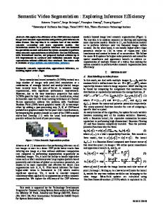
Illustration of these different shot transition techniques is shown in Figure 2. Shots are elementary to any kind of video analysis and video application as it facilitates segments of a video into its basic components. Shot transition detection (shot detection, cut detection) is subject to the automated detection of transitions between shots in digital video with the purpose of sequential segmentation of videos. The components of the shot boundary detection algorithms are (Cotsaces et al., 2006): •

Features used: to concentrate the large dimensionality of the video domain through extracting a small number of features from one/ more regions of interest (ROI) in each video frame.

The foremost methods for shot boundary detection are pixel differences, histogram comparisons, transform-based difference method, edge differences, and motion vectors. These methods can be discussed as follows (Deokar and Kabra, 2014). 1

Pixel comparison method: Two frames are taken as input and the intensity of pixels are to be calculated. If the intensity difference of pixels is above a certain threshold value, then scene change is declared. This method is moderately slow.

2

Histogram-based difference method: Computes the histogram of each frame and compares it to obtain the shot boundaries.

3

Transform-based difference method: Represents difference computation using different transformation methods such as the discrete cosine transformation (DCT).

4

Edge-based difference method: The edges of successive aligned frames are detected. Afterwards, the edge pixels are paired with close edge pixels in the other image to find out if any new edges have pierced the image or if some old edges have disappeared.

G. Pal et al.

6 5

Motion vector method: Find the vector fields for any image processing application. The changes in the image with time have appeared in the vector fields. •

Spatial feature domain: Refers to the size of the region from which features are extracted. It has an imperative role in the overall performance of shot change detection. A small region learns to reduce detection invariance with respect to motion. While a large region may direct to missed transitions between similar shots. Diverse possible choices can be; single pixel, rectangular block, arbitrarily shaped region, and whole frame.

•

Feature similarity metric: Is used to evaluate discontinuity between frames based on the selected features.

•

Temporal domain of continuity metric: Is used to select a temporal window that contains a representative amount of video activity to perform shot change detection. The window chosen can be: two frame window, N-frame window, or interval since the last shot change.

•

Shot change detection method: After computing a feature (or a set of features) on one or more ROI for each frame, a shot change detection algorithm is obligatory to detect where these reveal discontinuities. This is done using the following: static probabilistic detection, thresholding, adaptive thresholding, or trained classifier.

The rest of this work is organised as follows. Section 2 Introduce a literature review on the shot transition detection. While, Section 3 presents the proposed algorithm using minimum ratio similarity measurement. The simulation results are provided in Section 4. Finally, in Section 5 conclusion and future work are presented. Figure 2

Shot transition techniques (see online version for colours)

Video segmentation using minimum ratio similarity measurement

2

7

Literature review on shot transition detection

An accessible literature on video shot boundary detection methods are discussed as follows. Boreczky and Rowe (1996) evaluated the performance of different shot boundary detection and classification algorithms and their variations including histograms, DCT, motion vector, and block matching methods. The algorithm features used were region-based comparisons, running differences, and motion vector analysis. This work concludes that a combination of these three features produced better results than either the region histogram or the running histogram algorithms. Heng and Ngan (2001) introduced objects-based shot detection technique. This algorithm showed an improvement over previous popular algorithms. In the same year, Lee et al. (2001), proposed histogram comparison method-based shot detection algorithm. This method was not suitable for the condition where abrupt changes in luminance occur. A characteristic feature of video frames was used in Whitehead et al. (2004) that suggested an automatic threshold approach to detect an abrupt transition. Liu et al. (2004) provided a scheme for finding threshold using non-parameter-based constant false-alarm ratio (CFAR) processing technique to attain better precision and recall performance for cut detection. Binomial distributions were used in Su et al. (2005) to perceive dissolve transition. Where, an innovative dissolve-type transition detection algorithm that can accurately distinguish dissolves from disturbance caused by motion was presented. This work proposed model for dissolving then use it to filter out possible confusion caused by the effect of motion. Experimental results demonstrated the effectiveness of the proposed algorithm. Supervised SVM classifier used in Cao and Cai (2007) to detect a different digital video transition. The classifier classifies the frames in three different categories: a

abrupt change

b

gradual change

c

no scene change.

Another approach in Bezerra and Leite (2007) proposed a detection method of video transition using string matching techniques. An advanced technique was recommended to detect an abrupt transition using bipartite graph matching techniques as proposed in Guimaraes et al. (2009). A new improved rapid cut detection algorithm was recommended in Almeida et al. (2011). The experimental result showed an improvement over different algorithms. Pratim et al. (2012), proposed a shot change detection scheme by taking frame transition parameters and frame estimation errors based on global and local features. Fast video shot boundary detection based on segment selection, singular value decomposition (SVD) and pattern matching was suggested in Lu and Shi (2013). Anticipated a work on video shot boundary detection using dual-tree complex wavelet transform, an approach to process encoded video sequences prior to complete decoding was done in Mishra et al. (2013). The algorithm extracted the structure features from each video frame by using dual tree complex wavelet transform. Afterward, spatial domain structure similarity was computed between adjacent frames. An analysis and verification of video summarisation using shot boundary detection were illustrated in R and Shettar

G. Pal et al.

8

(2013). The analysis was standing on block-based histogram difference and block-based Euclidean distance difference for varying block sizes. Mishra et al. (2014) presented a comparative study of block matching algorithm and dual tree complex wavelet transform for shot detection in videos. As well as a comparison between the two detection methods in terms of various parameters such as hit rate, false rate, miss rate tested on a set of different video sequence was done.

3

Proposed algorithm for video segmentation using minimum ratio similarity measurement

The proposed system has three main steps as illustrated in the block diagram in Figure 3, and discussed as follows. Figure 3

Block diagram of proposed algorithm

Initially, different characteristic features of the frames are computed. These features are divided into four broad categories: spatial domain parameters, frequency domain texture parameters (Khazenie and Richardson, 1993), statistical texture parameters, edge information. These features can be described in details as follows.

3.1 Spatial domain parameters The different parameters in the spatial domain include calculation of the raw moments and central moments in R, G, and B planes, the mean and standard deviation of the intensities in each frame. Consider xi is the grey levels, fi is the pixel count of ith grey levels and N is the total number of the pixel of each image frame in the following discussion whereas in (Mohanta et al., 2013), a

Image raw moments: Is used to describe the motion about the origin. In the proposed algorithm, image raw moments up to third order have been used. •

The 1st order raw moment μ1' represents the mean of the pixel values of an image and the area of the image frames.

•

The 2nd order raw moment μ 2' is used to measure the variation of the pixel values of an image and the centroid of the image frame. The square root of the variance gives the standard deviation.

•

The 3rd order μ 3' raw moment is used to calculate the skewness of an image. Skewness is used for measuring the orientation and symmetry of the image. Image raw Moments can be calculated using the following equation:

Video segmentation using minimum ratio similarity measurement

μ n' =

1 N

255

∑x

n i

* fi

9

(1)

i =0

where, n is the order of the moment. b

Image central moments: The image central moments are used to identify spots/blobs on image individually central moments. It is calculated about the mean of the image frame. Image central moments tells whether two blobs are equal in terms of size, shape, orientation, which is in different parts of the image. It is used to find the orientation of a particular blob. Image central moments can be calculated as,

μn = c

∑ (x − μ )

' n 1

i

* fi

(2)

i =0

1 N

255

∑x * f i

(3)

i

i =0

Standard deviation in intensity: The standard deviation gives an idea of how close the entire set of pixel values of an image is to the average value. It measures the contrast of an image. The larger is standard deviation, the higher is the contrast. The standard deviation can be calculated using equation (4).

σ= e

255

Mean intensity: The arithmetic mean is a measure of the average intensity. The mean μ can be calculated using equation (3) as,

μ= d

1 N

⎡1 ⎢ ⎣⎢ N

⎤

255

∑ (x − μ ) * f ⎥⎦⎥ 2

i

i

Frequency domain texture parameters: Haar wavelet (Chui, 1992) is used for frequency domain texture analysis of the image frames. The Fourier transform is unable to represent a non-stationary signal. But time-frequency analysis function, Haar transform, is found more effective. Each R, G and B planes are transformed into one low-pass sub band (LL) and three high-pass sub bands (HL, LH and HH) using 2D Haar wavelet transform. In each of the three iterations, the same process applies to LL band. At each iteration the mean and standard deviation of ‘Haar’ wavelet coefficients of the high-pass sub bands are chosen as features. The Haar Wavelet’s mother wavelet function can be described by equation (5). 1 ⎫ ⎧ ⎪1 , 0 ≤ t < 2 ⎪ ⎪ ⎪ 1 ⎪ ⎪ ϕ (t ) ⎨− 1 , ≤ t < 1 ⎬ 2 ⎪ ⎪ ⎪0 , otherwise ⎪ ⎪ ⎪ ⎩ ⎭

f

(4)

i =0

Statistical texture parameters entropy (Song, 2008): Is used to measure the randomness of grey-level distribution in an image which indicates the texture variation. Equation (6) calculates the entropy as follows,

(5)

10

G. Pal et al. 255

Entropy =

i

i =0

g

⎛1⎞ ⎟ ⎟ i ⎠

∑ f × log⎜⎜⎝ f

(6)

Edge information: Edge detection is one of the essential difficulties with lower level image processing. It plays an indispensable role in the realisation of a complete vision-based understanding/monitoring system for automatic scene analysis/monitoring (Ahmad and Choi, 1999). Edge information is an apparent choice for characterising the ROI as it is sufficiently invariant to illumination changes and several types of motion. One of the characteristics feature presented in the frames is the High frequency components. Sobel operator is one of the efficient, high pass filters (Singh, 2014). It is based on computing an approximation of the gradient of the image intensity function. The 2D Sobel operator calculates the gradient along vertical and horizontal direction of the frames. The kernel of Sobel operator can be described as: ⎡− 1 − 2 − 1⎤ ⎡ − 1 0 1⎤ D x = ⎢⎢− 2 0 2⎥⎥, D y = ⎢⎢ 0 0 0 ⎥⎥ ⎢⎣ 1 ⎢⎣ − 1 0 1⎥⎦ 2 1 ⎥⎦

(7)

The filters Dx and Dy compute the gradient components across the neighbouring lines or columns, respectively. In the proposed work these different parameters are calculated for each frame that creates a feature vector of size 40 for each frame. Then, the feature vectors for two consecutive frames are used to find the similarity set between frames. Similarity set is described using eighteen similarity metrics, S = {si} where i = 1, 2, …, 18. Definitions of different similarity metric are given below: •

s1 represents the similarity between the raw moments of a red plane in two consecutive frames. It can be calculated using s1 = fs(V(i, 1:3), V(i + 1, 1:3)), where fs represents the similarity function, V represents the feature vector, i represents the frame number, and the column (1 to 3) of the feature vectors represents the first, second and third order raw moments in red plane; respectively.

•

s2 and s3 represent the similarity between the raw moments of green plane and blue plane in two consecutive frames. They can be calculated using column (4 to 9) of feature vectors which represent the first, second and third order raw moments in green and blue plane.

•

s4, s5 and s6 represent the similarity between the central moments of red, green and blue planes in two consecutive frames. These can be calculated using the column (10 to 18) of feature vectors which represents the first, second and third order central moments in red, green and blue plane.

•

s7 represents the similarity in grey plane in two consecutive frames. That can be calculated using the column (19 to 20) of feature vectors which represent the mean intensity and standard deviation between intensity in grey plane.

•

s8 to s16 represent the similarity in texture features in the frequency domain. s8 can be calculated using column (21 and 22) of feature vectors. This represents the mean and the standard deviation of the high-pass sub-band coefficients in the first iteration of the red plane.

Video segmentation using minimum ratio similarity measurement

11

•

Similarly, s9 and s10 can be calculated using the column number (23 to 26) which represent the mean and the standard deviation of the high-pass sub-band coefficients in the second and third iteration of red plane.

•

s11 to s16 can be calculated using the column (27 and 38) of feature vectors which represent the mean and standard deviation of the high-pass sub-band coefficients in the first, second and third iteration of green and blue plane; respectively.

•

s17 represents the similarity in statistical texture features between two consecutive frames. This can be calculated using column number 39 which represents the entropy of the frame.

•

s18 represents the similarity in edge information between two consecutive frames. This can be calculated using column number 40 which represents the area covered by the edges of the frame.

Consequently, the combination of similarity sets of the entire frame forms a similarity matrix of size [total frame number × 18]. The minimum ratio similarity measurement (Goshtasby, 2012) is used as a similarity function to calculate similarity between two given vectors. It performed best compared to other similarly measurement techniques (Acharjee et al., 2014). To clarify the minimum ratio similarity measurement concept, assume two vectors A = {A1, A2, A3, …} and B = {B1, B2, B3, …}. Then the similarity between A and B can be measured using the minimum ratio, which can be calculated using equation (8). mr =

1 n

n

⎛ Ai Bi ⎞

∑ min⎜⎜⎝ B , A ⎟⎟⎠ i =1

i

i

where n is the total size of the vector. Figure 4

Feature vector calculation (step 1)

(8)

12

G. Pal et al.

If two vectors are identical, then the minimum ratio attains maximum value 1. Lower value of minimum ratio indicates dissimilarity between vector A and B. Figure 4 shows the steps to calculate the characteristic features of every frame. Figure 5 shows the use of the calculated feature vector to calculate similarity sets and similarity matrix. Figure 5

Calculation of similarity set and matrix (step 2)

Finally, the characteristic features discussed are calculated for every frame at the initial step. The output of the initial step is a matrix with forty columns of different features and number of rows equal to the number of the total frames in the video. In a second step the similarity matrix calculated using the output of the first step. The similarity matrix is then used in step three to generate the decision matrix. The decision matrix contains binary values and equal to the size of the similarity matrix. If the similarity matrix of any frame indicates a significant change then the decision matrix will be true for the equivalent metric position. Else, the decision matrix will contain false value. In case the maximum matrix of a frame indicates a significant change, then that frame can be identified as shot transition boundary. Figure 6 illustrates the use of similarity matrix to detect the shot transition, which is the main core of step 3.

Video segmentation using minimum ratio similarity measurement Figure 6

Shot transition detection (step 3) S tart

In tia liz e D e cisio n M atrix o f size [T o talF ra m eN um b er,18 ] w ith 0 Initialize F ra m eC ou nte r= 1

Initialize Ite ra tion = 1

C re a te a w in do w o f 1 X N (N is od d n u m b er) in the sim ilarity m atrix w h ich w ill ran ge fro m [F ram e C o un ter-(N -1)/2,Iteration ] to [F ram eC o un te r+ (N -1)/2,Iteration ].

F ind the m inim a ins id e the w ind ow . L et the po sition o f th e m in im a inside the w in do w is k.

No

If k= {(N -1)/2}+ 1

Y es C alcu la te th e p erce nta ge of cha n ge in m a gn itud e o f v alue s in sid e w ind ow be tw e en (k-1 a nd k) p os itio n.A lso C a lcu la te the sam e p e rce nta ge of ch an ge in m a gn itud e b e tw ee n (k an d k+ 1 ) p ostio n

No

If B o th cha n ge >4% Y es

S et D e cisio n M atrix [F ram eC ou n te r,Itera tion ]= 1

Inc re ase Ite ra tio n b y 1

If Itera tion < = 1 8

Yes

No C o un t n u m b er of co lu m n ha s value 1 in the D e cision M a trix ro w nu m b e r [F ram eC o un te r].

If C o un t> 9

Yes S e t F ra m e F ra m e C o u nter as th e tran sitio n p oint b etw ee n tw o sho t

No

Inc re ase F ram e C ou nte r b y 1

If F ram e C o un ter < T o talF ra m e No S top

Yes

13

14

G. Pal et al.

4

Simulation results

Standard datasets with known ground truth are used for simulating the proposed algorithm. The test dataset (http://www.site.uottawa.ca/~laganier/videoseg/) used in Liu et al. (2004) and Pratim et al. (2012) for benchmarking. Here the video sample contains different types of quality and resolution. Different video samples with their type and quality levels are summarised in Table 1. Table 1

Details of test dataset

Sample name

Genres

Resolution

Total frame number

A

Cartoon

192 × 144

650

B

Action

320 × 142

959

C

Horror

384 × 288

1,619

D

Drama

336 × 272

2,632

E

Science fiction

384 × 288

536

F

Commercial

160 × 112

236

G

Commercial

384 × 288

500

H

Comedy

352 × 240

5,133

I

News

384 × 288

479

J

Action

240 × 180

873

The performance of the system is measured in terms of precision, recall and F-measure parameters where, •

Precision is the measurement that suggests the detected shots of the system are how much relevant.

•

Recall is the measurement which suggests how much correct shot boundaries are retrieved. Recall and precision are complementary metrics which cannot be used alone.

•

F-measure is combining the precision and recall.

The detected shot boundaries can be classified in four categories as shown in Table 2. Table 2

Categories of detecting shot boundaries True cut based on ground truth

True non-cut on ground truth

Classified as cut by algorithm

True positive (T+)

False positive (F+)

Classified as non-cut by algorithm

False negative (F–)

True negative (T–)

Based on the category of the detected shots precision, recall and F-measures metrics can be calculated using the following equations (9), (10) and (11).

Video segmentation using minimum ratio similarity measurement Precision = Recall =

F=

15

T+ T + + F+

T+ T + + F−

2 × Precision × Recall Precision + Recall

(9)

(10) (11)

The obtained result of the proposed algorithm is compared with six different methods: 1

rapid cut detection (Pratim et al., 2012)

2

histogram-based method (Pfeiffer et al., 1998)

3

pixel-based method with localisation (Liu et al., 2004)

4

feature tracking method (Liu et al., 2004)

5

visual rhythm with longest common subsequence (Guimaraes et al., 2009)

6

visual rhythm with clustering by k-means (Almeida et al., 2011).

The complete result is shown in Tables 3, 4 and 5 are discussed as follows. Table 3 demonstrates a comparative study of the precision metric. While, the proposed algorithm has the same average (AVG) precision value as the Histogram-based method, it is superior to all other algorithms as it has the maximum average precision. In addition to, it has the lowest standard deviation (DEV) compared to other algorithms for precision metric. This achieved result suggests that the precision performance of the algorithm is independent of the nature of the video. Table 4 summarises the comparison of the recall metric. The proposed algorithm has a very high precision which eventually leads to reduce the recall performance as recall and precision are complementary metrics. Table 4 shows the proposed algorithm performed better recall value rather than another algorithm such as the histogram-based method, visual rhythm with LCS, and pixel-based method with localisation, which have high precision values and less recall. Table 4 clearly shows that the obtained recall metrics for the proposed algorithms is not the highest amongst the benchmarked algorithms. As recall and precision are opposite metrics, another metric F-measure employed by combining the recall and precision metrics (Pratim et al., 2012). Table 5 shows the F-measure performance of all algorithms. The F-measure value is a single value that indicates the overall effectiveness of the image retrieval. The F-measure performance of the proposed algorithm is the best with maximum average value and minimum deviation among all other algorithms. Again the minimum standard deviation proves the robustness of the system.

1 1 0.89 1 0.96 1 1 0.95 1 0.91 0.971 0.042

B

C

D

E

F

G

H

I

J

AVG

DEV

0.048

0.971

0.85

1

0.971

1

1

0.955

1

0.936

1

1

P

P

A

Histogram based method (MOCA)

Proposed method uses minimum ratio similarity measurement

0.084

0.939

0.776

1

0.974

0.938

1

0.815

1

0.891

1

1

P

Rapid cut detection

0.185

0.874

0.497

1

0.895

0.81

1

0.938

1

0.595

1

1

P

Feature tracking method

0.181

0.857

0.683

1

0.949

0.95

1

0.828

1

0.662

0.5

1

P

Visual rhythm with k-means

0.301

0.771

0.623

1

0.927

0.708

0

0.867

1

0.764

0.825

1

P

Pixel based method with localisation

0.289

0.766

0.639

0.667

0.943

1

1

0.676

1

0.635

0.096

1

P

Visual rhythm with LCS

Table 3

Video sequence

16 G. Pal et al. Comparative study of precision metric

0.054

DEV

H

0.961

0.895

G

AVG

0.944

F

1

1

E

0.897

1

D

J

1

C

I

1 0.87

B

0.059

0.961

0.869

1

0.974

1

1

0.857

1

0.907

1

1

R

1

R

A

Visual rhythm with k-means

Feature tracking method

0.158

0.898

0.506

1

0.949

0.833

1

0.786

1

0.907

1

1

R

Rapid cut detection

0.151

0.863

0.64

1

0.8

0.83

1

0.80

0.95

0.61

1

1

R

Proposed method using minimum ratio similarity measurement

0.143

0.861

0.885

0.5

0.868

0.842

1

0.821

0.971

0.87

1

0.857

R

Visual rhythm with LCS

0.318

0.8

0.54

1

1

0.994

0

0.867

1

0.778

0.825

1

R

Pixel based method with localisation

0.246

0.701

0.395

0.5

0.895

0.667

1

0.7

0.941

0.536

0.375

1

R

Histogram based method (MOCA)

Table 4

Video sequence

Video segmentation using minimum ratio similarity measurement Comparative study of recall metric

17

1 0.868 1 0.751 0.91 0.105

H

I

J

AVG

DEV

E 0.907

0.872

D

G

0.974

C

F

1 0.723

B

0.127

0.91

0.612

1

0.961

0.882

1

0.800

1

0.899

1

1

F

1

F

A

Rapid cut detection

Proposed method using minimum ratio similarity measurement

0.134

0.908

0.637

1

0.895

0.872

1

0.968

1

0.707

1

1

F

Feature tracking method

0.126

0.898

0.765

1

0.961

0.974

1

0.842

1

0.766

0.667

1

F

Visual rhythm with k-means

0.179

0.794

0.54

0.667

0.932

0.8

1

0.808

0.969

0.682

0.545

1

F

Histogram based method (MOCA)

0.304

0.783

0.591

1

0.962

0.809

0

0.867

1

0.771

0.825

1

F

Pixel based method with localisation

0.249

0.769

0.742

0.571

0.904

0.914

1

0.742

0.985

0.734

0.176

0.923

F

Visual rhythm with LCS

Table 5

Video sequence

18 G. Pal et al. Comparative study of F-measure metric

Video segmentation using minimum ratio similarity measurement

19

Generally, the obtained result is not dependent on the content of the video. This result suggests that the proposed algorithm performed better than other algorithms in the comparison. Figures 7, 8 and 9 illustrate a comparative study of the precision, recall, and F-measure. Multiple variable graphs have been used to represent the result. The horizontal x-axis displays the variable names which are different compared algorithms, while the vertical y-axis represents value of metric. Metric values for different videos obtained for an algorithm are used to represent by the corresponding vertical line which also represents the range obtained by the algorithm. Uppermost point and lowermost point of the vertical line represent maximum and minimum value obtained by the algorithm. Dotted connecting lines connect the average value (AVG) obtained by every algorithm to indicate their relations. Figure 7 clarifies that either with different video samples, the proposed method has less variation of the precision values with different video samples. The obtained result in Figure 7 is matched with the same concluded from Table 3. As shown, the proposed method has the highest average precision with less variation compared to the other algorithms. While the worst case with maximum precision variation occurred when using the pixel-based method with localisation. Figure 7

Comparative study of precision metric for different video samples

1.0 0.8 0.6 0.4 0.2 Kmeans

LCS

FeatureTracking

PixelBased

MOCA

RapidCut

Proposed

0.0

Figure 8 clarifies that either with different video samples, the feature tracking method has less variation of the recall values with different video samples. Figure 8 result is matched with the same concluded from Table 4. While, the proposed method has the less average recall with more variation compared to the feature tracking method. But the proposed method has better recall compared to the algorithms with high precision value as mentioned in Table 4.

20 Figure 8

G. Pal et al. Comparative study of recall metric for different video samples

1.0 0.8 0.6 0.4 0.2 Kmeans

LCS

FeatureTracking

PixelBased

MOCA

RapidCut

Proposed

0.0

Figure 9 clarifies that the proposed method has less variation of the average F-measure values with different video samples. The result obtained in Figure 9 is matched with the same concluded from Table 5. While, the proposed method has the highest average Fmeasure with less variation compared to all other methods. Figure 9

Comparative study of F-measure metric for different video samples

1.0 0.8 0.6 0.4 0.2 Kmeans

LCS

FeatureTracking

PixelBased

MOCA

RapidCut

Proposed

0.0

Therefore, the simulation results prove that the proposed method has almost less variations of the metric average values, which indicates its robustness to the video samples used. These results indicate the efficiency of the proposed method using the minimum ratio similarity measurement compared to the benchmarked algorithms when measuring the precision and the F-measure metrics.

Video segmentation using minimum ratio similarity measurement

5

21

Conclusions and future work

Numerous algorithms have been proposed for detecting video shot boundaries and classifying shot and shot transition types. Shot detection is a challenging task due to its variety and diverse nature. This is the basic step towards automatic video indexing and browsing. There are diverse types of transitions or boundaries between shots. A cut is an abrupt shot change that occurs in a single frame. A fade is a slow change in brightness resulting in or starting with a solid black frame. A dissolve occurs when the images of the first shot get dimmer and the images of the second shot get brighter, with frames within the transition showing one image superimposed on the other. A wipe transpires when pixels from the second shot replace those of the first shot in a regular pattern such as in a line from the left edge of the frames. In this paper, an algorithm employed based on finding similarity between adjacent frames using spatial features and textures is proposed. The comparison of the proposed algorithm with another six different methods proves that it performed better rather than other algorithms having high precision value. Regarding the F-measure performance, the proposed algorithm is best with maximum average value and minimum deviation between all other algorithms. Thus, the proposed algorithm performed best in terms of precision and F-measure. The performance of the algorithm is not dependent on the content of the video which proves the robustness of the system. In future other similarity measurement techniques (i.e., correlation, MSE, etc.) can be used as a similarity function to replace minimum ratio similarity measurement technique. Also, the proposed system can be tested with medical videos.

References Acharjee, S., Chakraborty, S., Karaa, W., Azar, A and Dey, N. (2014) ‘Performance evaluation of different cost functions in motion vector estimation’, International Journal of Service Science, Management, Engineering, and Technology (IJSSMET), Vol. 5, No. 1, pp.45–65. Acharjee, S., Dey, N., Biswas, D., Das, P. and Chaudhuri, S. (2012a) ‘A novel block matching algorithmic approach with smaller block size for motion vector estimation in video compression’, 12th International Conference on Intelligent Systems Design and Applications (ISDA), pp.668–672. Acharjee, S., Dey, N., Biswas, D. and Chaudhuri, S. (2012b) ‘A novel block matching algorithmic approach with smaller block size for motion vector estimation in video compression’, International Conference on Intelligent Systems Design and Applications (ISDA-2012), Kochi, IEEE Xplore, 27–29 November. Acharjee, S., Dey, N., Biswas, D. and Chaudhuri, S. (2013) ‘An efficient motion estimation algorithm using division mechanism of low and high motion zone’, International Multi Conference on Automation, Computing, Control, Communication and Compressed Sensing (iMac4s-2013), Kerala, India, IEEE Xplore, 22–23 March. Ahmad, M. and Choi, T. (1999) ‘Local threshold and Boolean function based edge detection’, IEEE Transactions on Consumer Electronics, Vol. 45, No. 3, pp.674–679. Almeida, J., Leite, N. and Torres, R. (2011) ‘Rapid cut detection on compressed video’, Progress in Pattern Recognition, Image Analysis, Computer Vision, and Applications, Springer Berlin Heidelberg, pp.71–78.

22

G. Pal et al.

Araki, T., Ikeda, N., Dey, N., Acharjee, S., Molinari, F., Saba, L., et al. (2015) ‘Shape-based approach for coronary calcium lesion volume measurement on intravascular ultrasound imaging and its association with carotid intima-media thickness’, JUM, Vol. 34, pp.469–482, doi:10.7863/ultra.34.3.469. Bezerra, F. and Leite, N. (2007) ‘Using string matching to detect video transitions’, Pattern Analysis and Applications, Vol. 10, No. 1, pp.45–54. Boreczky, J. and Rowe, L. (1996) ‘Comparison of video shot boundary detection techniques’, Journal of Electronic Imaging, Vol. 5, No. 2, pp.122–128. Bose, S., Mukherjee, A., Madhulika, Chakraborty, S., Samanta, S. and Dey, N. (2013) ‘Parallel image segmentation using multi-threading and k-means algorithm’, 2013 IEEE International Conference on Computational Intelligence and Computing Research (ICCIC), Madurai, 26–28 December. Burke, B., Gregory, J., Cooper, M., Loomis, A., Young, D., Lind, T., et al. (2007) ‘CCD imager development for astronomy’, Lincoln Laboratory Journal, Vol. 16, No. 2, pp.393–412. Cao, J. and Cai, A. (2007) ‘A robust shot transition detection method based on support vector machine in compressed domain’, Pattern Recognition Letters, Vol. 28, No.12, pp.1534–1540. Chakrabarty, S., Pal, A.K., Dey, N., Das, D. and Acharjee, S. (2014c) ‘Foliage area computation using monarch butterfly algorithm’, 2014 1st International Conference on Non Conventional Energy (ICONCE), pp.249–253, doi: 10.1109/ICONCE.2014.6808740. Chakraborty, S., Acharjee, S., Bose, S., Mukherjee, A. and Dey, N. (2014b) ‘A semi-automated system for optic nerve head segmentation in digital retinal images’, 2014 International Conference on Information Technology, pp.112–117, doi: 10.1109/ICIT.2014.51. Chakraborty, S., Nath, S., Acharjee, S., Dey, N. and Roy, S. (2014a) ‘Effects of rigid, affine, b-splines and demons registration on video content: a review’, 2014 International Conference on Control, Instrumentation, Communication and Computational Technologies (ICCICCT), 10–11 July, pp.497–502, doi: 10.1109/ICCICCT.2014.6993013. Chui, C. (1992) An Introduction to Wavelets, Academic Press, San Diego, ISBN 0585470901. Cotsaces, C., Nikolaidis, N. and Pitas, I. (2006) ‘Video shot detection and condensed representation: a review’, IEEE Signal Processing Magazine, Vol. 23, No. 2, pp.28–37. Deokar, M. and Kabra, R. (2014) ‘Video shot detection techniques brief overview’, International Journal of Engineering Research and General Science, Vol. 2, No. 6, pp.817–820. Dey, N., Acharjee, S., Biswas, D., Das, A. and Chaudhuri, S. (2012a) ‘Medical information embedding in compressed watermarked intravascular ultrasound video’, Transactions on Electronics and Communications, Vol. 57, No. 71, pp.1–7. Dey, N., Das, P., Das, A. and Chaudhuri, S. (2012b) ‘DWT-DCT-SVD based intravascular ultrasound video watermarking’, Second World Congress on Information and Communication Technologies (WICT 2012), Trivandrum, India, October 30–November 02, IEEE Xplore. Dey, N., Maji, P., Das, P., Biswas, S., Das, A. and Chaudhuri, S.S. (2013) ‘An edge based blind watermarking technique of medical images without devalorizing diagnostic parameters’, 2013 International Conference on Advances in Technology and Engineering (ICATE), pp.1–5, doi: 10.1109/ICAdTE.2013.6524732. Dey, N., Roy, A. and Das, A. (2012c) ‘Optical cup to disc ratio measurement in glaucoma diagnosis using harris corner’, Third International Conference Computing Communication and Technologies 2012 (ICCCNT12), Coimbatore, July, IEEE Xplore. Dey, N., Roy, A., Pal, M. and Das, A. (2012d) ‘FCM based blood vessel segmentation method for retinal images’, International Journal of Computer Science and Network (IJCSN), Vol. 1, No. 3, pp.148–152. Dey, N., Roy, A.B., Das, P., Das, A. and Chaudhuri, S.S. (2012e) ‘Detection and measurement of arc of lumen calcification from intravascular ultrasound using Harris Corner detection’, 2012 National Conference on Computing and Communication Systems (NCCCS), pp.1–6, doi: 10.1109/NCCCS.2012.6413021

Video segmentation using minimum ratio similarity measurement

23

Gautam, P., Rudrapaul, D., Acharjee, S., Ray, R., Chakraborty, S. and Dey, N. (2015) ‘Video shot boundary detection: a review’, Emerging ICT for Bridging the Future – Proceedings of the 49th Annual Convention of the Computer Society of India CSI, Vol. 2, Advances in Intelligent Systems and Computing, Vol. 338, pp.119–127. Goshtasby, A. (2012) Similarity and Dissimilarity Measures, Image Registration, Springer London, pp.7–66. Guimaraes, S., Patrocinio, Z., Paula, H. and Silva, H. (2009) ‘A new dissimilarity measure for cut detection using bipartite graph matching’, International Journal of Semantic Computing, Vol. 3, No.2, pp.155–181. Guy, R. and Lownes-Jackson, M. (2013) ‘Web-based tutorials and traditional face-to-face lectures: a comparative analysis of student performance’, Informing Science and Information Technology, Vol. 10, pp.241–259. Heng, W. and Ngan, K. (2001) ‘An object-based shot boundary detection using edge tracing and tracking’, Journal of Visual Communication and Image Representation, Vol. 12, No. 3, pp.217–239. Ikeda, N., Araki, T., Dey, N., Bose, S., Shafique, S., El-Baz, A. et al. (2014) ‘Automated and accurate carotid bulb detection, its verification and validation in low quality frozen frames and motion video’, International Angiology, Vol. 33, No. 6, pp.573–89. Khazenie, N. and Richardson, K. (1993) ‘Comparison of texture analysis techniques in both frequency and spatial domains for cloud feature extraction’, International Archives of Photogrammetry and Remote Sensing, Vol. 29, pp.1009–1009. Lee, M., Yang, Y. and Lee, S. (2001) ‘Automatic video parsing using shot boundary detection and camera operation analysis’, Pattern Recognition, Vol. 34, No. 3, pp.711–719. Liu, T., Lo, K., Zhang, X. and Feng, J. (2004) ‘A new cut detection algorithm with constant false-alarm ratio for video segmentation’, Journal of Visual Communication and Image Representation, Vol. 15, No. 2, pp.132–144. Lu, Z. and Shi, Y. (2013) ‘Fast video shot boundary detection based on SVD and pattern matching’, IEEE Transactions on Image Processing, Vol. 22, No. 12, pp.5136–5145. Mishra, R., Singhai, S. and Sharma, M. (2013) ‘Video shot boundary detection using dual-tree complex wavelet transform’, 2013 IEEE 3rd Advance Computing Conference (IACC). Mishra, R., Singhai, S. and Sharma, M. (2014) ‘Comparative study of block matching algorithm and dual tree complex wavelet transform for shot detection in videos’, 2014 International Conference on Electronic System, Signal Processing and Computing Technologies (ICESC). Mohanta, P., Saha, S. and Chanda, B. (2013) ‘A novel technique for size constrained video storyboard generation using statistical run test and spanning tree’, International Journal of Image and Graphics, Vol. 13, No. 1, pp.1–24, DOI:10.1142/S0219467813500010. Ngan, K and Li, H. (Eds.) (2011) Video Segmentation and Its Applications, Springer Science and business Media. Springer, London. Noldus, L., Spink, A. and Tegelenbosch, R. (2001) ‘EthoVision: a versatile video tracking systemfor automation of behavioral experiments’, Behavior Research Methods, Instruments, & Computers, Vol. 33, No. 3, pp.398–414. Pfeiffer, S., Lienhart, R., Kühne, G. and Effelsberg, W. (1998) The MoCA Project – Movie Content Analysis Research at the University of Mannheim, in J. Dassow and R. Kruse (Eds.) Informatik ’98, Springer Verlag Berlin, Heidelberg, pp.329–338. Pratim, P., Saha, S. and Chanda, B. (2012) ‘A model-based shot boundary detection technique using frame transition parameters’, IEEE Transactions on Multimedia, Vol.14, No. 1, pp.223–233. R, S. and Shettar, R. (2013) ‘Analysis and verification of video summarization using shot boundary detection’, American International Journal of Research in Science, Technology, Engineering & Mathematics, Vol. 3, No. 1, pp.82–86.

24

G. Pal et al.

Roy, P., Goswami, S., Chakraborty, S., Azar, A. and Dey, N. (2014) ‘Image segmentation using rough set theory: a review’, International Journal of Rough Sets and Data Analysis (IJRSDA), IGI Global, Vol. 1, No. 2, pp.1–13. Samanta, S., Acharjee, S., Mukherjee, A., Das, D. and Dey, N. (2013) ‘Ant weight lifting algorithm for image segmentation’, 2013 IEEE International Conference on Computational Intelligence and Computing Research (ICCIC), Madurai, 26–28 December. Samanta, S., Dey, N., Das, P., Acharjee, S. and Chaudhuri, S. (2012) ‘Multilevel threshold based gray scale image segmentation using cuckoo search’, International Conference on Emerging Trends in Electrical, Communication And Information Technologies – ICECIT, pp.27–34. Singh, S., Saurav, S., Saini, R., Saini, A., Shekhar, C. and Vohra, A. (2014) Comprehensive Review and Comparative Analysis of Hardware Architectures for Sobel Edge Detector, Hindawi Publishing Corporation Electronics 2014. Song, M. (2008) Entropy Encoding in Wavelet Image Compression. Representations, Wavelets, and Frames Applied and Numerical Harmonic Analysis, pp 293–311, doi: 10.1007/978-0-81764683-714. Su, C., Liao, H., Tyan, H. and Fan, K. (2005) ‘A motion-tolerant dissolve detection algorithm’, IEEE Transactions on Multimedia, Vol. 7, No. 6, pp.1106–1113. Whitehead, A., Bose, P. and Laganiere, R. (2004) ‘Feature based cut detection with automatic threshold selection’, Image and Video Retrieval, Springer Berlin Heidelberg, pp.410–418.