Secondly, im- age quality is rather low, especially in terms of the colors. Another, but much smaller database has been produced by. Koudelka et al. [10]. Hence ...
Viewpoint Consistent Texture Synthesis Alexander Neubeck, Alexey Zalesny, and Luc Van Gool Swiss Federal Institute of Technology Zurich Computer Vision Lab {aneubeck,zalesny,vangool}@vision.ee.ethz.ch
Abstract The purpose of this work is to synthesize textures of rough, real world surfaces under freely chosen viewing and illumination directions. Moreover, such textures are produced for continuously changing directions in such a way that the different textures are mutually consistent, i.e. emulate the same piece of surface. This is necessary for 3D animation. It is assumed that the mesostructure (small-scale) geometry of a surface is not known, and that the only input consists of a set of images, taken under different viewing and illumination directions. These are automatically aligned to build an appropriate Bidirectional Texture Function (BTF). Directly extending 2D synthesis methods for pixels to complete BTF columns has drawbacks which are exposed, and a superior sequential but highly parallelizable algorithm is proposed. Examples demonstrate the quality of the results.
1. Introduction Textures are often used to convey an impression of surface detail, without having to invest in fine-grained geometry. Starting from example images, several methods can model textures and synthesize more extended areas of them [1, 4–7, 13, 14, 16] A shortcoming of early methods was that these textures would remain fixed under changing viewing or lighting directions, whereas the 3D structures they were supposed to mimic would lead to changing self-occlusion and shadowing effects. Therefore, more recent texture modeling and synthesis methods include such effects [3,8,10–12,15], with some of our own work as an early example [18, 19]. These recent methods can be used to cover curved surfaces with textures that adapt their parameters to the different, local orientations with respect to the viewpoint and light sources. The gain in realism when compared to fixed texture foreshortening and shading is often striking. Animations, where the viewpoint or light sources move with respect to the surface, add the requirement of texture
consistency over time. Subsequent textures for the same surface patch should seem to all visualize the same physical surface structure. Only a subset of the previous methods can produce such consistent time series of textures. Examples are those which explicitly retrieve surface height or normal information [3, 12] or stitch together texton representations that already include their appearance under several viewing conditions [11, 15] and where the ‘textons’ can shrink to a single pixel [8, 10]. Both approaches limit the geometric complexity that can be handled. For the former this immediately stands to reason, but it may be less obvious for the latter. We will return to this issue shortly. In this paper we propose a novel method of the latter type, i.e. based on a kind of copy-and-paste approach. It tries to overcome the limitations of current methods, by widening the choice of basic material to copy from without the need for additional sample images. Also, we deal with real, colored textures, rather than synthetic or grey level ones, as has sometimes been the case. The paper is organized as follows. Section 2 describes the input images that we use, as well as the way in which the incoming information is organized. Section 3 describes the texture synthesis method that exploits this information to produce consistent textures. Section 4 shows examples. Section 5 concludes the paper.
2. Bidirectional Texture Function 2.1. Images stacks as input The input consists of images of a planar sample of the texture, taken under known viewing conditions (known viewing and illumination directions). The biggest publicly available image database of this kind is the CUReT [2], which has some insufficiencies. Firstly the representation is not complete because for each illumination direction there is only a 1D trajectory of viewing angles. Secondly, image quality is rather low, especially in terms of the colors. Another, but much smaller database has been produced by Koudelka et al. [10]. Hence, we have constructed a spe-
Figure 2. Stack alignment. Left: oblique view, middle: oblique view after alignment to frontal view, right: frontal view.
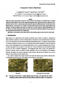
Figure 1. Setup for taking pictures under variable viewing and illumination directions.
Figure 3. Lichen texture. left: frontal view, right: oblique cially designed apparatus, shown in Fig. 1. It consists of a camera arm that can be moved to specified inclinations, several light sources that can be individually activated, and a turntable on which the texture sample is placed. The arm and table rotate about orthogonal axes, thereby covering a complete hemisphere of directions. The sessions are computer controlled, so that the user only needs to specify desired intervals. All images are then taken automatically at the desired angular resolutions, except for the illumination directions, which are limited by the light sources present in the setup. There have been only 4 lamps so far, but many more are planned in the follow-up version of the setup. We plan to make the texture data available [17]. Starting from the different images the bidirectional texture function or ‘BTF’ can be constructed. The BTF representation was introduced by Dana et al. [2]. It contains the intensities or colors observed for a certain point (specified by its ‘texture coordinates’) on the texture, for each viewing and lighting directions. Hence, it is a 6D function. In practice this function is sampled by thousands of images taken under different illumination and viewing directions, hence the need for a largely automated setup as just described. These images are rectified by projective transformations, to let their outlines precisely fit those of the frontal view. The determination of the transformations is facilitated by a set of markers placed around the texture patch on the turntable. Fig. 2 shows two images of the same texture (an oblique view on the left and the frontal view on the right). The image in the middle is the image on the left, projectively aligned with the frontal view on the right. Such alignment
view.
is part of the automatic image capturing procedure. This alignment removes the global, perspective distortions. We will refer to the complete set of aligned images of a texture as a BTF stack. When only the data at a fixed pixel location is considered, we refer to the corresponding data subset as a BTF column. One such BTF column of the “lichen” texture example of Koudelka et al. [10] (Fig. 3) is visualized in Fig. 4. The same pixel intensities are shown twice, using two different orderings of the imaging conditions. Each small block of the top image consists of pixels ordered according to the two viewing angles, whereas the blocks themselves are or-
Figure 4. BTF column visualization (cutout). Top: each block represents tilt/pan angles of viewing direction, blocks are arranged by tilt/pan angles of lighting direction. Bottom: Switched viewing and lighting angles in the ordering.
view 2
view 1
view 1
view 2 view 1
view 2
dered according to the two lighting angles. In the bottom image the roles of viewing and lighting are swapped. Already at first glance it is clear that the intensities within the blocks are smoother when they are arranged by lighting angles. This has to do with the 3D nature of the real surface: changing only the lighting and keeping the viewing direction fixed ensures that also in such case a fixed pixel in the images will correspond to one fixed point on the surface. In case the viewing direction is changed, alignment through a simple planar projectivity cannot avoid that the same pixel will now correspond to different points on the surface, thereby increasing the changes in intensities. Smoothness in the BTF is important, as it improves the creation of intermediate views. BTF-based rendering is usually based on pixelwise linear interpolation between nearest views. The more similar these neighboring views are, the better it works. The same holds for the synthesis of entirely novel texture patches by smart copy-and-pasting of BTF data (a strategy used in e.g. [8, 10]). Seamless knitting based on smooth functions is easier than for functions with lots of variation. This brings us to an issue that has not received much attention yet, but that has an important impact on the usefulness of BTF stacks. Due to the 3D nature of most real textures, the BTF is not unique. So far images were aligned to the coplanar markers on the turntable, but a similar alignment based on parallel planes at different heights yields different BTFs for exactly the same texture patch. BTF smoothness can be increased by making an optimal choice. This is discussed next.
projection planes
drift
texture surface
Figure 5. Nonuniqueness of BTF representation. A surface point is mapped to distinct pixels in the BTF. The pixel drift depends on the projection plane position.
by nearby views, it can be skipped. The smoothness is maximized by choosing the alignment plane which minimizes the average Euclidean distance between the intensities of neighboring views sharing the same lighting direction. That is, the appearance change is measured as a pixelwise Euclidean distance with respect to the four neighboring camera positions. The average value of this Euclidean distance over the whole BTF stack is calculated for several plane positions within a reasonable range. The plane corresponding to the minimal distance is chosen. In Section 4 we show an example of the beneficial influence that such selection of the alignment plane has on the quality of the rendering (Fig. 10).
2.3. Column vs. view-specific BTF copying 2.2. Improved BTF Alignment As mentioned in the last section, the BTF representation of a texture is not unique, as it depends on the choice of the alignment plane. This choice will also have an influence on the smoothness of the BTF, and therefore on its potential for texture synthesis. As mentioned, the alignment to a reference plane (like that of the turntable markers) cannot avoid that the same pixel will correspond to different physical points on the surface (texture sample). This drift is illustrated in Fig. 5. If not all surface points lie in the same plane, images taken under different viewing directions cannot be aligned to map all points onto each other, even under the simplifying assumption of parallel projection. On the other hand, drift effects can be minimized and thus BTF smoothness increased by aligning with respect to a plane within the height range of the texture. For texture synthesis based on copy-and-pasting of BTF data – which is also the basis of the approach presented in this paper – it stands to reason that a good BTF stack is one with maximal smoothness. Such stack could also support further subsampling: if a view can be interpolated very well
Suppose we extend a smart copying type of texture synthesis for single views [1, 4, 5, 13, 16] to complete BTF columns, i.e., complete BTF columns are copied and pasted instead of RGB values (like in [8, 10]), based on their compatibilities with already synthesized parts of the texture. It would be extremely difficult to avoid strong seams, except for very regular textures. This can be explained as follows. Consider the simple artificial texture shown in Fig. 6 (left). It was created by the superposition of Gaussian functions, that are assumed to simultaneously specify surface height and intensity. They were centered at the nodes of a randomly deformed grid and also their widths (standard deviations) were randomly chosen. For this surface the BTF stack was generated by orthogonal projections. Due to the 3D nature of the texture, BTF columns will always comprise information about a neighborhood rather than a single surface point. Differently shaped Gaussians have spots with similar orientations and would therefore share similar BTF columns if this information mixing would not occur. But as BTF columns are bound to combine information from several surface points,
Figure 6. Artificial texture. Left: original, middle: copy-and-paste applied to complete BTF columns, right: result of a per-view copy-and-paste synthesis.
differently shaped Gaussians will no longer share any BTF column. A single BTF column already contains sufficient data to reconstruct the Gaussian blob it was sampled from. As all these Gaussians have different shapes, their BTF columns will not be easy to combine. Hence, except for verbatim copying of large chunks – which is often undesirable and would still result in seams between these chunks – it is nontrivial to make neighboring columns consistent and thereby avoid seams. Chances of forming new Gaussian shapes are slim. The result of a copy-and-paste strategy (see section 3.1) applied to complete BTF columns for this example is shown in the middle image of Fig. 6. The higher complexity of real surfaces only worsens the problem. It will be very improbable to find two BTF columns in a rough irregular texture patch, which share the same reflectance properties for all viewing and lighting directions. This makes synthesis by copying whole BTF columns almost impossible. Although the choice of an appropriate alignment plane reduces the problem of finding compatible BTF columns, this will not suffice. Taking much larger texture samples and therefore increasing the number of BTF columns to choose from can also remedy this problem to some extent, but is not always practical. Thus, on top of alignment plane optimization we propose an alternative strategy to enlarge the choice of samples. The proposed approach no longer copies and pastes complete BTF columns, but only the data from the BTF that are relevant for a specific viewing condition, i.e. only a small part of the BTF. Hence, rather than synthesizing all views simultaneously, they are created one by one. Initially, a single view is synthesized, which can be done with any traditional texture synthesis algorithm. Then, this so-called support view is used to guide the synthesis of the other views. In our experiments we have always used a frontal view as the support view, but this is not necessary. The support view has to ensure that the different textures are consistent. The small part of the BTF columns that is used consists of the data
(intensity or color) for the support view and of the desired view (different viewing and or lighting directions). Now only small parts of the BTF columns need to be compatible, thereby drastically increasing the choice, as we will combine parts from different columns to synthesize the corresponding pixel in different views. The price clearly is a loss in efficiency, but the quality of such procedure is superior, as is shown in Fig. 6(right) for the artificial example with the Gaussians. There are no longer seams visible, while simultaneously the variation in acceptable hill shapes has increased. During this sequential synthesis two contradicting issues must be solved: texture quality and viewpoint consistency. On the one hand seams might be better hidden when there are more choices of stitching patches together. On the other hand, requiring view consistency still amounts to restricting the choice. The intuition behind our approach is similar to Image Analogies [9]: given the original frontal view A, its viewpoint consistent oblique view B and a synthetic frontal view A′ (the support view), the synthetic oblique view B ′ has to be created in a way consistent with A′ . From a BTF column, only the entries from A and B are used. The copyand-paste process is led both by consistency with a pixel’s neighborhood in the fixed support A′ and the data already available in the corresponding neighborhood within the B ′ view under construction. As the synthesis of B ′ proceeds, a dynamic weighting scheme increases its influence in this comparison. After carrying out such synthesis for the different possible views B ′ , a complete stack can be build again, where the BTF columns are no longer one-to-one copies of original BTF columns. Instead, they are compositions of several columns, thereby yielding many more possibilities. Fig. 7 compares columnwise synthesis (left) with our sequential approach (right) for a real colored white-pea texture. Columnwise synthesis again produces more salient seams.
input texture
output texture
(p+u,q+v) (p,q)
Figure 7. Left: columnwise synthesis; There are salient
(i+u,j+v) (i,j)
seams visible. Right: sequential synthesis.
3. Synthesis Algorithm Figure 8. Candidate neighborhood selection for syntheAs described in the previous section our sequential synthesis scheme first synthesizes a single view, the support view, and then the remaining ones. Therefore first the details of the single view synthesis are explained.
3.1. Single View Synthesis Our single view synthesis algorithm combines the non-parametric multiscale texture synthesis of Paget and Longstaff [13], which samples from an example image to build a similar output texture, with Ashikhmin’s candidate search [1]. The latter reduces the search complexity for similar neighborhoods by introducing a reasonable subset of possible candidates from the example image. At the start the output image – which is to become the support view – is randomly initialized such that its histogram equals the histogram of the input image. Then a pixel of the output image is randomly chosen and a set of possible candidate pixels in the input image is created (this will be explained shortly). Next the neighborhood of the chosen output pixel is compared to the neighborhoods of all the candidates. It is replaced by the intensity (or color) of the input candidate pixel with the best matching neighborhood. This procedure is repeated until all output pixels were visited a number of times. Now follow more details. To fill the chosen pixel of the output pixel with an intensity (or color), its neighborhood is investigated in order to select good candidate values from the input sample. More precisely, input pixels are identified that have at least one intensity (or color) in their neighborhood that is identical and in the same relative neighborhood position. This is illustrated in Fig. 8). The input pixel neighborhood with the smallest Euclidean distance between the intensities (or RGB-values) of its pixels and the corresponding ones of the output pixel under scrutiny is considered to match best. The output pixel is updated and takes on the intensity (or color) of the input pixel with this neighborhood. As a matter of fact, the updating procedure is iterative and when visiting a pixel anew it is only updated if an input pixel with a better matching neighborhood is found.
sis.
To guide the updating procedure, a ‘confidence’ is assigned to each output pixel. It specifies the chance of the pixel to be selected for an update. The higher the confidence, the lower this chance gets. Basically, the confidence counts the number of previous updates a pixel has undergone, as this number gives a good idea of how. The confidence values w(i, j) for all pixels (i, j) are initialized to zero. Whatever the outcome, a constant value is added to the pixel’s confidence: w(i, j) := w(i, j) + 1/T,
(1)
where T is the total number of times each pixel will be visited (as a rule T = 4). A pixel with confidence 1 will no longer be selected or updated. The chance to be selected for a possible update is X (1 − w(i′ , j ′ )), (2) P (i, j) = (1 − w(i, j))/ (i′ ,j ′ )∈Image
where w(i, j) ∈ [0, 1] is the confidence of pixel (i, j) and P (i, j) is the visiting probability. The confidences also have a second role to play. The more confidence we have in a pixel is, the more it contributes to the Euclidean distance in the comparison between the input and output neighborhoods: P dist(i, j, p, q) = (u,v)∈N w(i + u, j + v) · ||out(i + u, j + v) − in(p + u, q + v)||2 ,
(3)
where the neighborhood N = � (u, v)|0 < u2 + v 2