Billings and Chen, 1998). These produce linear or non- linear polynomial functions that model the relation- ship between some input and some output, both per-.
Visual Task Identification Using Polynomial Models∗ T. Kyriacou1 , O. Akanyeti1 , U. Nehmzow1 , R. Iglesias2 and S.A. Billings3 1 Dept. of Computer Science, University of Essex, UK. 2 Electronics and Computer Science, University of Santiago de Compostela, Spain. 3 Dept. of Automatic Control and Systems Engineering, University of Sheffield, UK. Abstract Developing robust and reliable control code for autonomous mobile robots is difficult, because the interaction between a physical robot and the environment is highly complex, subject to noise and variation, and therefore partly unpredictable. This means that to date it is not possible to predict robot behaviour based on theoretical models. Instead, current methods to develop robot control code still require a substantial trial-and-error component to the software design process. This paper proposes a method of dealing with these issues by a) establishing task-achieving sensor-motor couplings through robot training, and b) representing these couplings through transparent mathematical functions that can be used to form hypotheses and theoretical analyses of robot behaviour. In the spirit of the FIFA World Cup 2006 we demonstrate the viability of this approach by teaching a mobile robot to track a moving football, using the Narmax system identification technique.
1.
Introduction
The behaviour of a robot (for example the trajectory of a mobile robot) is influenced by three components: i) the robot’s hardware, ii) the program it is executing and iii) the environment it is operating in. Because this is a complex and often non-linear system, in order to program a robot task to achieve a desired behaviour, one usually has to resort to empirical trial-and-error processes. Such iterative-refinement methods are costly, time-consuming and error prone (Iglesias et al., 2005). One of the aims of the RobotMODIC project is to establish a scientific, theory-based, design methodology for robot control program development. As a first step towards this aim we “identify” a robot’s behaviour, using system identification techniques such as ARMAX (Auto-Regressive Moving Average models with eXogenous inputs) (Eykhoff, 1974, Eykhoff, 1981) and NARMAX (Nonlinear ARMAX) (Chen and Billings, 1989, ∗ Proc.
“Towards Autonomous Robotic Systems”, Taros 2006
Billings and Chen, 1998). These produce linear or nonlinear polynomial functions that model the relationship between some input and some output, both pertaining to the robot’s behaviour. The representation of the task as a transparent, analysable model enables us to investigate the various factors that affect robot behaviour for the task at hand. For instance, we can identify input-output relationships such as the sensitivity of the robot’s behaviour to particular sensors (Roberto Iglesias and Billings, 2005), or make predictions of behaviour when a particular input is presented to the robot. This, we believe, is a step towards the development of a theory of robot-environment interaction that will enable a more focused and methodical design of robot controllers.
1.1
Identification of visual sensor-motor competences
In previous work (Iglesias et al., 2004, Iglesias et al., 2005, Nehmzow et al., 2005) we presented and analysed models for mobile robot tasks that used the laser and sonar rangefinder sensors as input modalities. Tasks included wall-following, obstacle avoidance, door traversal and route-learning. In this paper we show how the same modelling methodology can be applied for tasks using the vision sensor (video camera) on our robot. The task that we model here is one where the robot follows a bright orange ball in an open space of more or less uniform grey colour. We use the NARMAX methodology (described briefly in section 2.2) in order to model this task.
2.
Experimental procedure and methods
2.1
Experimental procedure
The experiments described in this paper were conducted in the 100 square metre circular robotics arena of the University of Essex, using a Magellan Pro mobile robot called Radix (figure 1). The robot is equipped with 16 sonar, 16 infra-red and 16 tactile sensors uniformly distributed around it. A SICK laser range finder is also present, this range sensor scans the front semi-circle of the robot ([0◦ , 180◦ ]) with a radial resolution of 1◦ and a
distance resolution of less than 1 centimetre. The robot also incorporates a colour video camera on a pan/tilt platform. For the purposes of the work presented here only the video camera was used.
Figure 2: An example of a robot camera image (left) and its coarse-coded version (right). Note that the coarse-coded image is shown enlarged by a factor of 20.
ing the rotational velocity of the robot as a function of the colour of each of the pixels in coarse-coded camera image. A brief explanation of the model estimation procedure used is given in the following section.
2.2
The NARMAX modelling methodology
The NARMAX modelling approach is a parameter estimation methodology for identifying both the important model terms and the parameters of unknown nonlinear dynamic systems. For multiple input, single output noiseless systems this model takes the form: Figure 1: Radix, the Magellan Pro mobile robot and the orange-coloured ball used in the experiments described in this paper.
y(n)
=
f (u1 (n), u1 (n − 1), u1 (n − 2), · · · , u1 (n − Nu ), u1 (n)2 , u1 (n − 1)2 , u1 (n − 2)2 , · · · , u1 (n − Nu )2 , ··· , u1 (n)l , u1 (n − 1)l , u1 (n − 2)l , · · · , u1 (n − Nu )l ,
Acquisition of estimation and testing data In order to collect data for the estimation of the task model a human driver manually drove the robot using a joystick, guiding the robot to follow a moving orange ball (see figure 1) . The driver used only the robot’s camera images to steer the robot towards the ball. The robot’s camera was tilted to its lower extreme so that the robot’s field of view covered the area closest to the robot. The robot was driven for 1 hour. During this time a coarse-coded robot camera image and the robot’s translational and rotational velocities were logged every 250 ms. The camera image was coarse-coded to a minimal 8x6 pixel image by averaging neighbourhoods of 20x20 pixels in the original 160x120 pixel image. Figure 2 shows an example of a camera image and its coarsecoded version. Coarse-coding of the camera image was done for two reasons: (a) in order to minimise hard disk access and memory requirements during the robot’s operation and (b) to reduce the dimensionality of the input to the NARMAX model. After the collection of the model estimation and validation data a polynomial model was obtained, identify-
u2 (n), u2 (n − 1), u2 (n − 2), · · · , u2 (n − Nu ), u2 (n)2 , u2 (n − 1)2 , u2 (n − 2)2 , · · · , u2 (n − Nu )2 , ··· , u2 (n)l , u2 (n − 1)l , u2 (n − 2)l , · · · , u2 (n − Nu )l , ··· , ··· , ud (n), ud (n − 1), ud (n − 2), · · · , ud (n − Nu ), ud (n)2 , ud (n − 1)2 , ud (n − 2)2 , · · · , ud (n − Nu )2 , ··· , ud (n)l , ud (n − 1)l , ud (n − 2)l , · · · , ud (n − Nu )l , y(n − 1), y(n − 2), · · · , y(n − Ny ), y(n − 1)2 , y(n − 2)2 , · · · , y(n − Ny )2 , ··· , y(n − 1)l , y(n − 2)l , · · · , y(n − Ny )l )
were y(n) and u(n) are the sampled output and input signals at time n respectively, Ny and Nu are the regression orders of the output and input respectively, d is the dimension of the input vector and l is the degree of the polynomial. f () is a non-linear function and here taken
to be a polynomial multi-resolution expansion its arguments. Expansions such as multi-resolution wavelets or Bernstein coefficients can be used as an alternative to the polynomial expansions considered in this study. The first step towards modelling a particular system using a NARMAX model structure is to select appropriate inputs u(n) and the output y(n). The general rule in choosing suitable inputs and outputs is that there must be a causal relationship between the input signals and the output response. After the choice of suitable inputs and outputs, the NARMAX methodology breaks the modelling problem into the following steps: i) polynomial model structure detection, ii) model parameter estimation and iii)model validation. The last two steps are performed iteratively (until the model estimation error is minimised) using two sets of collected data: (a) the estimation and (b) the validation data set. Usually a single set that is collected in one long session is split in half and used for this purpose. The model estimation methodology described above forms an estimation toolkit that allows the user to build a concise mathematical description of the input-output system under investigation. These procedures are now well established and have been used in many modelling domains (Billings and Chen, 1998). A more detailed discussion of how structure detection, parameter estimation and model validation are done is presented in (Korenberg et al., 1988, Billings and Voon, 1986).
3.
Experimental results
We used the Narmax system identification procedure to estimate the robot’s rotational velocity as a function of 144 inputs (the red, green and blue values of each of the 8x6 pixels of the coarse-coded camera image), using the data obtained during the ball-following experiment. The model was chosen to be of first degree and no regression was used in the inputs and output (i.e. l = 1, Nu = 0, Ny = 0), i.e. a linear ARMAX polynomial structure. The resulting model contained 53 terms: ω(n)
= +0.1626308495 +0.0028080424 ∗ u8 (n) −0.0016263169 ∗ u14 (n) −0.0025145629 ∗ u15 (n) ... +0.0061225193 ∗ u129 (n) −0.0051800999 ∗ u136 (n) +0.0012762243 ∗ u144 (n)
where ω(n) is the rotational velocity of the robot in
rad/s at time instant n and {ui |i ∈ Z, 1 ≤ i ≤ 48}, {ui |i ∈ Z, 49 ≤ i ≤ 96}, {ui |i ∈ Z, 97 ≤ i ≤ 144} are the red, green and blue components (respectively) of the coarse-coded image pixels (starting from the top left of the image and reading from left to right each image row). A graphical representation of the model parameters is given in figure 3. This figure shows the contribution of each coarse-coded image pixel to the rotational velocity ω(tn ). This contribution is obviously dependent on the colour value of the pixel at time tn . Inspection of figure 3 (and especially the red channel bar graph, which displays how the model will react to the near-red ball colour) reveals that the robot will tend to turn to the left (negative rotational velocity) when a red object like the ball appears to the left of the camera image, and vice versa. Interestingly, by looking at the green channel bar graph we can also postulate that the robot will tend to turn away from a green-coloured object. A quick laboratory test with Radix confirmed this hypothesis. Testing the model In order to test the model systematically, we performed a dynamic and a static test. In the dynamic test the ball was moved continuously in the field of view of the robot while the model controlled the robot. During this test the translational velocity of the robot was clamped to 0.15 m/s. The test was run for approximately 5 minutes, during this time the rotational velocity of the robot and the full resolution images recorded by its camera were logged every 250 ms. Figure 4 shows the average rotational velocity of the robot corresponding to the location of the ball in the (coarse-coded) image during the test run. To quantify the response of the robot in relation to the location of the ball, we computed the Spearman rank correlation coefficient between the angle-to-the-ball (from the robot’s perspective)1 and the robot’s rotational velocity for the entire test run. This was found to be 0.63 (sig., p