IEEE TRANSACTIONS ON IMAGE PROCESSING, VOL. 12, NO. 6, JUNE 2003
639
Visualization of High Dynamic Range Images Alvaro Pardo, Student Member, IEEE, and Guillermo Sapiro, Member, IEEE
Abstract—A novel paradigm for information visualization in high dynamic range images is presented in this paper. These images, real or synthetic, have luminance with typical ranges many orders of magnitude higher than that of standard output/viewing devices, thereby requiring some processing for their visualization. In contrast with existent approaches, which compute a single image with reduced range, close in a given sense to the original data, we propose to look for a representative set of images. The goal is then to produce a minimal set of images capturing the information all over the high dynamic range data, while at the same time preserving a natural appearance for each one of the images in the set. A specific algorithm that achieves this goal is presented and tested on natural and synthetic data. Index Terms—High dynamic range, visualization.
I. INTRODUCTION IGH dynamic range images contain a wide range in luminance, many times in the order of tens of thousands different values.1 These images could be natural, obtained for instance from multi-exposure photographs [1] or with a multiple exposure sensor [2], [3], or synthetic, in the case of computer graphics applications. These images have ranges that greatly exceed that of the output device. The question is then how can we reproduce and visualize such images in a standard output/viewing device. We address this problem in this paper. Before proceeding, let us introduce some basic terminology. The scene is the real or synthetic picture we perceive without involving any output device between it and our eyes.2 An image, on the other hand, is what we can see using the output device, or its internal computer representation as an array of digital values. The key problem is how to translate from scenes to images while preserving the relevant scene information, producing a natural looking image and avoiding common artifacts such as halos, which are due to local gradient reversals [4]. Numerous applications exist for high dynamic range images. One is computer graphics and the production of synthetic im-
H
Manuscript received August 14, 2001; revised January 29, 2003. This work was supported in part by the Office of Naval Research under Grant ONR-N00014-97-1-0509, the Office of Naval Research Young Investigator Award, the Presidential Early Career Awards for Scientists and Engineers (PECASE), a National Science Foundation CAREER Award, the National Science Foundation Learning and Intelligent Systems Program (LIS), and CSIC—Universidad de la República, Uruguay. The associate editor coordinating the review of this manuscript and approving it for publication was Dr. Mark S. Drew. A. Pardo is with the IMERL & IIE, Facultad de Ingeniería, Universidad de la República, CC-30, Montevideo, Uruguay (e-mail:
[email protected]). G. Sapiro is with the Electrical and Computer Engineering, University of Minnesota, Minneapolis, MN 55455 USA (e-mail:
[email protected]). Digital Object Identifier 10.1109/TIP.2003.812373 1These
images are also referred in the literature as high contrasted. the case of synthetic scenes, it might be sometimes very difficult to directly visualize the data. 2In
ages with realistic or hyper-realistic appearance. Another application covers high dynamic range photographs, which are able to capture much more detailed scene information than standard photographs. Recently, methods to acquire such photographs have been developed [1]–[3]. These systems make it possible to capture a highly detailed range representation of the scene and later process the data in order to select the image/s that better fulfills the given requirements. These images could also improve computer vision and image analysis algorithms that usually rely on limited range data. This is particularly relevant in scenarios where we do not have complete control over the illumination, like medical applications for instance. Therefore, there is a need to develop algorithms to perform the translation from scenes to images, algorithms as the ones discussed and presented in this paper. We can classify the existing approaches for the translation from scene to image in two main groups (examples of these will be detailed in the next section). The first group consists of algorithms that map the original range to the output range while attempting to preserve the subjective perception of the scene, e.g., [5]. Although this idea of “tone mapping” works quite well, it has some caveats. First, it is not able to reproduce all the details present in the scene. Second, the method breaks down when the input range is too wide (and uniform) compared with the available output range. In the second group, we have algorithms that favor the visualization of details instead of the subjective perception of the scene. As examples of this approach we have the works of Tumblin and Turk [6] and DiCarlo and Wandell [4]. Both apply a multiscale decomposition to discriminate between illumination and details. The main problem with this idea is that, although correct in theory, it usually introduces halos in the output image. The local mappings produced by these techniques violate the basic monotonicity principle, the pixel value order is not necessarily preserved and darker (brighter) regions in the scene might become brighter (darker) in the image. Moreover, these approaches tend to have a large number of parameters, generally hard to control in an automatic fashion. Our proposed paradigm attempts to have the best of both groups mentioned above. We propose a method that captures the details while preserving the natural appearance of the scene. As we will explain below, there is an intrinsic limitation in representing a high dynamic range image with only one standard output image. Sometimes it is practically impossible to find an output image containing all the relevant information in the high dynamic range image that represents the scene. For this reason, we argue for a method to obtain a set of images containing all the relevant information of the original scene and displayed in a suitable way. This set also includes a single satisfactory image that can be used if the specific application is
1057-7149/03$17.00 © 2003 IEEE
640
limited to a single output. In general, different applications can select different subsets from the output of our algorithm. Our proposed approach is particularly useful when the high dynamic range image contains detailed information in regions with very different light levels, thereby requiring the use of different images to accurately visualize each region. This will be exemplified with our experiments. Our paradigm is also of particular use when the display device effortless permits the use of multiple images. This is the case for example of electronic displays and less the case of printed media. A. Related Work In [7], Tumblin and Rushmeier developed a tone mapping operator using models of human perception. The main drawback of their algorithm is that they use a global brightness adaptation, dark and bright regions are clipped. Schlick [8] concentrated on a simple method for computing a local tone mapping. Ferweda et al. [9] noted the connection between light levels, color, and acuity. Using this work, Larson et al. [5] proposed a global tone mapping operator which adjusts the histogram of the scene based on psychophysical models for color, glare, and acuity perception. The results of this simple and elegant method, which reduces to just a global map, are very good and with high fidelity to the subjective perception of the scene. The problem is, as for most of the methods in this category, when the input range is too large and the scene histogram is already near uniform (the algorithm does perform well when the histogram is bimodal with a large gap between the modes). Note that since this method tries to preserve the original perception of the scene, details that are hard to see in the original scene will be difficult to see in the output image as well. In [10], the authors introduce two methods to display high dynamic range images. The first one is intended to display synthetically generated images. The image is decomposed into layers of lighting and surface properties. The light layer, which contains most of the high contrast, is compressed and added back to the surface layers containing details and texture. In this way, high contrast is reduced while preserving the details and texture from the original image. This method is designed to work only for synthetic images, for which the different layers are easily computed. (We will come back to this point later when reviewing the work of Tumblin and Turk [6].) For natural scenes, they proposed a locally adaptive method, denoted as the foveal display, which is inspired by eye movements. The user selects a point of attention and the algorithm computes an output image with preserved contrast in the foveal region (a region around the selected point). It is important to remark that this approach is dynamic in the sense that a set of images is generated with the aid of user interaction. The drawback with this approach is that the user needs to select a point of attention. Moreover, the user should be able to “see” everywhere in the image to choose the points of attention. Problems could then arise if the image presented to the user is not adequate for inspection. On the other hand, we should note that this approach is connected to ours in the sense that we also suggest to compute a set of images instead of a single one. The work of Pattanaik et al. [11] proposes a multiscale model for the representation of pattern, luminance and color in the
IEEE TRANSACTIONS ON IMAGE PROCESSING, VOL. 12, NO. 6, JUNE 2003
human visual system. The main problem with this work is that, although interesting for its detailed modeling of the human visual system, it cannot avoid halos. Similar to the work of Pattanaik et al., we have the multiscale generalization [12], [13] of the Retinex algorithm [14]. In this approach, to avoid the appearance of halos close to strong edges [13], is necessarily to finely tune the weighting of the different scales [12]. In terms of dynamic range compression, it performs well for moderate dynamic range compression but not for high dynamic range compression [12]. Continuing with the idea of segregating the image into layers of lighting and details [10], Tumblin and Turk [6] proposed a multiscale approach to extract a hierarchy of details and boundaries. Their idea is to mimic the way artists work from coarse to fine when recreating highly contrasted scenes in low contrasted mediums. Artists start with a sketch of strong features and progressively add small details. They propose to decompose the image into strong and weak features using a multiscale operator, then, only strong features are compressed. Although the idea is very attractive, their algorithm cannot avoid halos completely and, as pointed out by the authors, needs the difficult tuning of some crucial parameters. In our view of the problem, the two groups of works just described are not completely equivalent; they basically address slightly different problems. Furthermore, although similar, their solutions cannot be easily compared, since one representation tries to capture the global subjective appearance of the scene under the limitation of the output/display device, while the second group attempts to visualize the scene details (note that details may be difficult to see even in front of the scene). While enhancing details, we may be adding information not perceptually present in the original scene. On the other hand, while preserving visual appearance, details might be omitted. Let us conclude by pointing out that recently, the authors in [15] have shown how to obtain panoramic images with high dynamic range. B. Our Contribution The approaches described above produce a single image per scene or per focused scene region. It is quite an optimistic assumption that we can accurately represent and visualize the information of an image with tens of thousands of values and with details in regions with very different luminance, with just one image and with limited dynamic range. This is what motivates the paradigm here proposed, meaning the use of a set of images to represent such highly detailed information. We could say that while the algorithms described above deal with the reproduction of the scene, the technique here proposed deals with its visualization. Moreover, we argue that not only the set of images has to accurately visualize the relevant information present in the scene, but also has to do it in a visually pleasant form. We present a particular algorithm to exemplify this new paradigm. In the proposed algorithm, each image is produced by a different monotonic global map, thereby avoiding gradient reversals typical of the local schemes. The locality is achieved by letting this global map “stretch” different regions for each one of the images in the set.
PARDO AND SAPIRO: VISUALIZATION OF HIGH DYNAMIC RANGE IMAGES
641
we first display dark regions expanding its luminance range and then we slowly swap resources to bright areas. This simple idea resembles the control of illumination during acquisition and is perceived as natural by human observers. A. Outline of the Algorithm
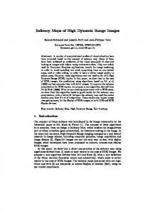
Fig. 1. Illustration of the idea of compression/expansion of the luminance range. A linear mapping from the input range [L ;L ] to the output range [L ;L ] and the piecewise linear one are shown. In our case, we will substitute each linear segment with the mapping proposed by Larson et al. (see Section II-A).
II. THE METHOD Our idea is to propose a simple and effective method to visualize all the information in the scene in a pleasant way. All means that we would like to capture as many details as possible and pleasant means a procedure which appears natural to the observer. Finally, we address the problem of halos and other artifacts in the solution. Let us assume we have a scene with dark and bright areas and details all over it. If we want to visualize all the details we need first to have a minimum dynamic range available and second to be able to “see” in every region. In order to understand what is meant by “see,” we present a couple of simple examples. Consider dark room, in order to “see” the details we would usually turn on the lights. Now, suppose we are in the beach and everything is too bright, in this case to “see” we would probably wear sunglasses to reduce the amount of light. In both cases, the information is out there but it cannot be seen. In photographic terms, this is due to under-exposure or over-exposure. These problems are not at all new, especially in photography they are of great importance. If we take a picture of an object and there is light coming from behind it, we will not capture all its details. To solve this, photographers put extra light to the front of the object. We are going to borrow this idea and modify the luminance of the scene to capture all the details over it. All the proposed operations are simply contrast changes. In this way, artifacts such as halos are not introduced. The first observation is that if we modify a region’s luminance, expanding its range of variation, it will be easier to perceive details in it. On one hand we display this region with “good illumination,” while on the other hand we might be compressing and missing details in other regions. In Fig. 1 we show a piecewise linear mapping which illustrates our idea. Hence, there is clearly a competition between the output fidelity of different regions and unfortunately, it is difficult or impossible to find a satisfactory solution with a single output. To overcome this, we propose to generate a sequence of images with different resolutions in each scene region (space varying resolution). This sequence could be either observed as a movie or as a set of still images could be extracted from it. The key point here is that for many applications more than one output image is a reasonable solution. The basic idea is then to distribute the existing resources among different output images. In the case of only two regions,
Before presenting our proposed algorithm, let us give some basic notation: ( ) Input color primaries. Input luminance. , ] Input luminance range. [ Modified luminance. , ] Output luminance range. [ ) Digital output values. ( We are now ready describe the different steps of the algorithm. ) primaries 1) Compute scene luminance: From the ( compute the luminance (in cd/m ) and the color infor). We process the luminance while mation ( preserving the color information. 2) Segment the scene: Divide the scene into two or more regions of interest. This is achieved splitting the histogram into subintervals . If we segment the scene arbitrary we could loose the monotonic restriction of the tone mapping. We then choose a simple procedure that segments the scene into bright and dark areas to illustrate the idea, see Section III-A. From now on then, in this section, we ] and [ ]. assume two regions, [ 3) Modify the luminance: Apply Larson et al.’s histogram adjustment algorithm, [5], to each interval. ] to [ ] and [ ] Map [ ]. This algorithm computes the output to [ with the formula3 brightness
where is computed from the cumulative freto quency distribution of the input brightness guarantee that the output image does not exhibit contrast that is more noticeable than it would be in the real scene. This is done constraining the slope of the operator using an estimation of the just noticeable differences ) for a given adaptation luminance level. That ( is, the slope of the operator is constrained to the ratio of the just noticeable differences at world and display ). We refer levels ( the reader to [5] for the details on the implementation of this mapping. Is important to note that since Larson’s , it is algorithm modifies the original distribution not a traditional histogram equalization algorithm. close to we will It is clear that if we select ], with a wider be visualizing the dark areas, [ we range than the bright ones. Thus, by changing modify the resources assigned to each interval of the original luminance. A first solution to the problem of visualization high dynamic range data is to create a movie by 3The display brightness is computed as display luminance.
B
= log(L ) where
L
is the
642
IEEE TRANSACTIONS ON IMAGE PROCESSING, VOL. 12, NO. 6, JUNE 2003
decreasing from to . This gives us a sequence, which starting from the image with all resources allocated to the dark areas, slowly moves to an image with all resources allocated to the bright areas. This is just a nice way of visualizing all the information. A second possibility is to choose just a certain fixed number of images. We discuss below how to select these images. In the case of three intervals or more, the idea is the same. We start with most resources allocated to the first interval and then we swap them to the next interval to the right. That is, we first split the output luminance range into three intervals, , with and . Initially, is much greater . Then we decrease the first interval in and than increase the second one in the same amount. That is, we swap resources form the first interval to the second one, obtaining the intervals . We iterate this procedure until the step when and then we proceed to do the same with the second and third intervals. Note that in the examples in this paper we use Larson et al.’s histogram adjustment algorithm for demonstration purposes, although other approaches can be used. That is, once the intervals have been obtained, other techniques can be applied to each one (as long as they preserve the order and avoid halos, a property we consider crucial in HDR visualization). We found that considering its very low complexity, Larson’s approach produces very good results. 4) Compute the output color primaries: Recompute the ). Instead color primaries ( of using the previous formula, to control the color saturation, we can compute a compressed dynamic range image ) with beusing ( tween 0.4 and 0.6 [6]. To find the output digital images we use the radiance library [16] but any other rendering method can be used. This library permits the correction of color in the mesopic and scotopic range, however, due to the luminance modification we applied, this modification usually does not take place.
III. ESTIMATION OF THE NUMBER OF IMAGES The minimal number of images needed for a satisfactory visualization of all the details in the high dynamic range data depends on the luminance distribution within the given scene. Therefore, to obtain an estimation of the number of output images we use the number of clusters in the luminance histogram.4 To display the scene without loss of information we would need, roughly, as many output levels as clusters present in it. However, not all output levels can be used if we want to distinguish between them. That is, we should use less output levels in order to guarantee that different input levels are mapped into visually different output levels. We use an empirical rule of thumb that says that we can allocate around 200 clusters per image in the set. This is just a coarse estimation that works fairly well in practice. Having an estimation of the number of output images required to satisfactory visualize the scene information, segmentation is needed in order to find the location of the luminance intervals. Obtaining a good segmentation in this case is a difficult problem. To begin with, we want to visualize information even in places where there is not enough (or too much) light and standard segmentation algorithms will fail to segment these regions properly since bright and dark spots will be typically assigned to a single region. Second, it is hard to obtain segmentations with regions matching our perception. We then select a simple approach based on the histogram. If needed, the user can correct the segmentation according with his/her needs. In what follows, we explain this segmentation procedure. A. Histogram-Based Segmentation The segmentation method we propose to use has been satisfactory used for documents in order to separate text from background. The text is made of dark pixels while the bright ones represent the background. To segregate the text from the background, a threshold that maximizes the sum of the entropy of of both distributions is computed. Given the probabilities of bright pixels, is computed maximizing dark pixels and the entropy
B. Information Assessment As we mentioned before, the evaluation of the output image is mostly subjective. However, it would be of interest to have an automatic procedure to assess the information content of each image in the set. With it, we will be able to extract the best or set of best images in the sequence. If we consider each image as a message, its information can be measured with its entropy. We can therefore use this as a plausible measure of the image information. From the histogram of the output image we find the probabilities of each output level and with them we compute the entropy. Note the relation between histogram equalization and entropy. The entropy is maximum when all symbols are equally probable, which implies a flat histogram. We have experimentally observed that entropy maximization captures our subjective preference toward well-contrasted images.
In our case we want to separate dark and bright regions. Using the histogram of the luminance and computing the above probabilities we apply a full search method to find the threshold that optimally segments dark and bright areas. If we use only two images, we only need to apply this procedure once; otherwise, we iterate this scheme. Using the estimation of output images and the segmentation algorithm described above we split the image into regions. This procedure can be seen as a binary tree construction, where in each step an interval is divided in two. At the end, the user can select the important leaves from it if user interaction is constructed in the process. 4We compute the number of clusters using the algorithm for peak detection proposed in [17].
PARDO AND SAPIRO: VISUALIZATION OF HIGH DYNAMIC RANGE IMAGES
643
Fig. 2. (a) Segmented image into three regions and (b) the original image with a linear tone mapping. Note how the segmentation based on the histogram provides a good partition; the dark and bright areas are clearly segmented. Also, note how a linear map saturates bright areas. In the rest of the image we show for each region we display the image with maximum entropy in the region. Images that visualize (c) region 0, (d) region 1, and (e) region 2. (f) Image obtained with Larson’s algorithm.
IV. RESULTS We now present a number of examples of our proposed algorithm. For the examples here presented, no user intervention was needed and the number of images and segmentation was performed as explained above. Movies showing the full set for the examples below and others can be found at http://mountains.ece.umn.edu/~guille/web-hdr/hdr.html. The first example is shown in Fig. 2. This high dynamic range image was captured by Devebec and Malik [1]. Before discussing the results obtained for this example, we give specifics on the parameters of the algorithm.
The first step is the segmentation of the original image [see Fig. 2(a)]. We found 419 clusters in the image luminance and therefore we use three output images (since we consider no more than 200 clusters per image). The intervals where found applying twice the algorithm described in Section III-A. First, we obtained a segmentation of bright and dark areas and then we subsegmented again the dark interval. Details of the segmentation are given in Table I. Second, we assign the given resources cd/m and to each region. In this case we assumed cd/m and selected initial ranges cd/m and cd/m . For the next image in the set, the resources are re-allocated moving them from left to right in steps
644
IEEE TRANSACTIONS ON IMAGE PROCESSING, VOL. 12, NO. 6, JUNE 2003
Fig. 3. (a) Image processed with Larson’s algorithm. (b) Image with maximum global entropy among all the images computed. Note how this image shows more details.
Fig. 4. Zoomed images for: (a) Fig. 2(c), (b) Fig. 2(d), (c) Fig. 2(e), and (d) Fig. 2(f). TABLE I INFORMATION FOR MEMORIAL CHURCH IMAGE
of cd/m (see the above mentioned web page for the full set of images obtained). From the data in Table I we can draw several conclusions. To begin with, the first regions have very small luminance values.
This means that is very difficult, even being in front of the real scene, to perceive details there. The dynamic range for this region is extremely small, representing only the 5.32 10 of the total input range. In other words, although region 0 covers a significant part of the scene, it expands an insignificant range from the total. Once again, it is clear that high dynamic range data it is not just a problem of output range, it is in fact a problem of resolution within regions in the scene. In Fig. 2(c)–(e), we show the set of images obtained with our algorithm. Each image represents the image with maximal entropy per region. With these images we can see more details
PARDO AND SAPIRO: VISUALIZATION OF HIGH DYNAMIC RANGE IMAGES
645
Fig. 5. Zoomed images for (a) Fig. 2(c), (b) Fig. 2(d), (c) Fig. 2(e), and (d) Fig. 2(f) computed with Larson’s algorithm.
Fig. 6.
Zoomed images for (a) Fig. 7(b), (b) Fig. 7(c), and (c) Fig. 7(f).
than in the single image processed with Larson’s algorithm (see Fig. 2(f) and also Fig. 3). The resulting images in Fig. 2(c)–(e) are fairly natural, specially for the last two images. The three
images selected visualize more information, especially in very dark and very bright regions. Hence, we managed to display the original scene in a set of images, making visible some informa-
646
IEEE TRANSACTIONS ON IMAGE PROCESSING, VOL. 12, NO. 6, JUNE 2003
Fig. 7. (a) Segmented image. (d) Image with a linear tone mapping. In the other images we show for each region, the image with maximum entropy in the region. Images that visualize: (b) region 0 and (c) region 1. (e) Image with maximum global entropy. (f) Image obtained with Larson’s algorithm.
tion that was obscured in the original scene. Note for example the details in the dark corners and in the bright windows. In the first image, Fig. 2(c), observe the upper left and upper right corners; the details in the ceiling are clearly visible now. In the second, Fig. 2(d), image observe the walls. Finally, the third image, Fig. 2(e), represents the windows. Note how we make visible the details in the windows. These areas are completely lost with a linear tone mapping (simple linear map of the input range onto the output range); see Fig. 2(b). The visualized details are also richer than those obtained with a Larson’s single output image, Fig. 2(f). Since our method extends Larson’s one, among all the images in the set, there should be one image close to the one obtained with Larson’s algorithm. In other words, if we resign to use more than one image and visualize all the details in the scene, we should be able to extract a single satisfactory one from the computed set. This is important, since the proposed technique not only permits a better visualization of the details using multiple images, Fig. 2, but also provides a single satis-
factory image in case the output device is limited to a single image. That is, the set of produced images includes one image that can be used as single output data, as in classical HDR problems. Different applications can pick different subsets from the data produced by our algorithm, including a single output. To select a single image from the set, we consider the image that maximizes the global entropy. If we compare it with the image computed with Larson’s algorithm, see Fig. 3, we can see that it contains enough details everywhere. This is due to the modification of the luminance distribution; we expanded regions that were originally very compressed. However, it is clear from the zoomed images, Figs. 4 and 5, that it does not capture dark and bright details as well as the images with maximum resources per region. The same methodology was applied to the bathroom image. Here we selected two regions ([3,262] cd/m , [299, 177 222]cd/m ). Fig. 7(a) shows the segmented image and Fig. 7(d) the image obtained with a linear tone mapping. In this case, although the number of computed clusters indicated
PARDO AND SAPIRO: VISUALIZATION OF HIGH DYNAMIC RANGE IMAGES
the use of three images in the set, we selected only two regions of the decomposition since they correctly represent the image. cd/m , For this image the algorithm parameters are cd/m and cd/m . The image with all resources allocated to the bright region captures in a better way the details in the lamps while the one with all resources in the dark region accurately captures details in the rest of the scene, see Figs. 7 and 6. Finally, the image with maximum global entropy, Fig. 7(e), balances both regions and is comparable with the image obtained by Larson’s algorithm, Fig. 7(f). V. CONCLUSIONS In this paper, we have presented a new paradigm for the reproduction and visualization of information in high dynamic range images. We argued for the use of a set of images instead of a single one as in traditional approaches. This is particularly important when the image contains details in regions with very different illumination. The set of produced images also includes a single image that is satisfactory for applications limited to a single output. More than being the last word about the problem of visualizing high dynamic range data, with this work we attempted to illustrate the intrinsic limitation of working with only one image. We showed how going for more than one image we could obtain a simple and nice solution to the problem of complete information visualization of high dynamic range images. A number of questions remain open after this work. The specific algorithm here described for the computation of the set of images is just a particular example and others should be developed. One of the crucial additional points is how to find the minimal number of images required to visualize all the relevant information. These images have also to be pleasant and hopefully with smooth transitions among them. We hope that the work here presented will open the door to works on these and other relevant questions. ACKNOWLEDGMENT The bathroom images were obtained from http://positron.cs. berkeley.edu/gwlarson. The authors thank J. Tumblin for explaining his work [6] and M. Bertalmio for fruitful discussions. REFERENCES [1] P. Debevec and J. Malik, “Recovering high dynamic range radiance maps from photographs,” in SIGGRAPH 97 Conf. Proc., 1997, pp. 369–378. [2] S. Nayar and T. Mitsunaga, “High dynamic range imaging: Spatially varying pixel exposures,” in Proc. IEEE Conf. Computer Vision and Pattern Recognition, vol. 1, June 2000, pp. 472–479. [3] B. Wandell, P. Catrysse, J. DiCarlo, D. Yang, and A. E. Gamal, “Multiple capture single image architecture with a CMOS sensor,” in Proc. Int. Symp. Multispectral Imaging and Color Reproduction for Digital Archives, 1999, pp. 11–17. [4] J. DiCarlo and B. Wandell, “Rendering high dynamic range images,” Proc. SPIE, vol. 3965, Jan. 2000. [5] G. W. Larson, H. Rushmeier, and C. Piatko, “A visibility matching tone reproduction operator for high dynamic range scenes,” IEEE Trans. Visual. Comput. Graph., vol. 3, pp. 291–306, Oct./Dec. 1997.
647
[6] J. Tumblin and G. Turk, “LCIS: A boundary hierarchy for detail-preserving contrast reduction,” in SIGGRAPH 99 Conf. Proc., 1999. [7] J. Tumblin and H. Rushmeier, “Tone reproduction for realistic images,” IEEE Comput. Graph. Applicat., vol. 13, pp. 42–48, Nov. 1993. [8] C. Schlick, “Quantization techniques for visualization of high dynamic range pictures,” in Photorealistic Rendering Techniques, Proc. 5th Eurographic Rendering Workshop, June 1994, pp. 7–20. [9] J. Ferwerda, S. Pattanaik, P. Shirley, and D. Greenberg, “A model of visual adaptation for realistic image synthesis,” in SIGGRAPH 96 Conf. Proc., 1996, pp. 249–258. [10] J. Tumblin, J. Hodgins, and B. Guenter, “Two methods for display of high contrasted images,” ACM Trans. Graphics, vol. 18, no. 1, pp. 56–94, Jan. 1999. [11] S. Pattanaik, J. Ferwerda, M. Fairchild, and D. Greenberg, “A multiscale model of adaptation and spatial vision for realistic image display,” in SIGGRAPH 98 Conf. Proc., 1998, pp. 287–298. [12] Z. Rahman, D. Jobson, and G. Woodell, “A multiscale retinex for color rendition and dynamic range compression,” Proc. SPIE, vol. 2847, 1996. [13] D. Jobson, Z. ur Rahman, and G. Woodell, “Properties and performance of a center/sorround retinex,” IEEE Trans. Image Processing, vol. 6, pp. 451–462, Mar. 1997. [14] E. Land and J. McCann, “Lightness and retinex theory,” J. Opt. Soc. Amer., vol. 63, no. 1, pp. 1–11, 1971. [15] Y. Y. Schechner and S. K. Nayar, “Generalized mosaicing,” in Proc. IEEE Int. Conf. Computer Vision, 2001, pp. 369–378. [16] Radiance [Online]. Available: htp://radsite.lbl.gov/radiance/HOME. html [17] J.-O. Eklundh and A. Rosenfeld, “Peak detection using difference operators,” IEEE Trans. Pattern Anal. Machine Intell., vol. PAMI-1, pp. 317–325, July 1979.
Alvaro Pardo (S’00) was born in Montevideo, Uruguay, in 1975. He received the Electrical Engineer degree from the Universidad de la República of Uruguay (UdelaR) in 1998. During 1999 and 2000, he was a visiting postgraduate student at Center of Vision Speech and Signal Procesing at the Unversity of Surrey, U.K. He also has been a visitor at the University of Minnesota, Minneapolis. He is currently pursuing the Ph.D. degree at Faculty of Engineering—UdelaR. He works as an assistant at the Departments of Mathematics and Electrical Eng. at the Faculty of Engineering, UdelaR.
Guillermo Sapiro (M’95) was born in Montevideo, Uruguay, on April 3, 1966. He received the B.Sc. (summa cum laude), M.Sc., and Ph.D. degrees from the Department of Electrical Engineering at The Technion—Israel Institute of Technology, Haifa, in 1989, 1991, and 1993 respectively. After postdoctoral research at MIT, he became Member of Technical Staff at the research facilities of HP Labs, Palo Alto, CA. He is currently with the Department of Electrical and Computer Engineering at the University of Minnesota, Minneapolis. He works on differential geometry and geometric partial differential equations, both in theory and applications in computer vision, computer graphics, medical imaging, and image analysis. He co-edited a special issue of the Journal of Visual Communication and Image Representation. He has authored and co-authored numerous papers in this area and has written a book published by Cambridge University Press in January 2001. Dr. Sapiro co-edited a special issue of the IEEE TRANSACTIONS ON IMAGE PROCESSING. He was awarded the Gutwirth Scholarship for Special Excellence in Graduate Studies in 1991, the Ollendorff Fellowship for Excellence in Vision and Image Understanding Work in 1992, the Rothschild Fellowship for Post-Doctoral Studies in 1993, the Office of Naval Research Young Investigator Award in 1998, the Presidential Early Career Awards for Scientist and Engineers (PECASE) in 1988, and the National Science Foundation Career Award in 1999. He is a member of SIAM.