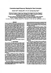
In other words, the speech signal uttered by a first speaker, ... unique correct conversion result: when a speaker utters a given sentence multiple times, each ..... number of free parameters grows quadratically with the input dimensionality.
0 5 Voice Conversion Jani Nurminen1 , Hanna Silén2 , Victor Popa2 , Elina Helander2 and Moncef Gabbouj2 2 Tampere University
1 Accenture of Technology Finland
1. Introduction Voice conversion (VC) is an area of speech processing that deals with the conversion of the perceived speaker identity. In other words, the speech signal uttered by a first speaker, the source speaker, is modified to sound as if it was spoken by a second speaker, referred to as the target speaker. The most obvious use case for voice conversion is text-to-speech (TTS) synthesis where VC techniques can be used for creating new and personalized voices in a cost-efficient manner. Other potential applications include security related usage (e.g. hiding the identity of the speaker), vocal pathology, voice restoration, as well as games and other entertainment applications. Yet other possible applications could be speech-to-speech translation and dubbing of television programs. Despite the increased research attention that the topic has attracted, voice conversion has remained a challenging area. One of the challenges is that the perception of the quality and the successfulness of the identity conversion are largely subjective. Furthermore, there is no unique correct conversion result: when a speaker utters a given sentence multiple times, each repetition is different. Due to these reasons, time-consuming listening tests must be used in the development and evaluation of voice conversion systems. The use of listening tests can be complemented with some objective quality measures approximating the subjective rating, such as the one proposed in (Möller, 2000). Before diving deeper into different aspects of voice conversion, it is essential to understand the factors that determine the perceived speaker identity. Speech conveys a variety of information that can be categorized, for example, into linguistic and nonlinguistic information. Linguistic information has not traditionally been considered in the existing VC systems but is of high interest for example in the field of speech recognition. Even though some hints of speaker identity exist on the linguistic level, nonlinguistic information is more clearly linked to speaker individuality. The nonlinguistic factors affecting speaker individuality can be linked into sociological and physiological dimensions that both have their effect on the acoustic speech signal. Sociological factors, such as the social class, the region of birth or residence, and the age of the speaker, mostly affect the speaking style that is acoustically realized predominantly in prosodic features, such as pitch contour, duration of words, rhythm, etc. The physical attributes of the speaker (e.g. the anatomy of the vocal tract), on the other hand, strongly affect the spectral content and determine the individual voice quality. Perceptually,
70
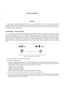
2
Speech Enhancement, Modeling and Recognition – Algorithms and Applications Will-be-set-by-IN-TECH
the most important acoustic features characterizing speaker individuality include the third and the fourth formant, the fundamental frequency and the closing phase of the glottal wave, but the specific parameter importance varies from speaker to speaker and from listener to listener (Lavner et al., 2001). The vast majority of the existing voice conversion systems deal with the conversion of spectral features, and that will also be the main focus of this chapter. However, prosodic features, such as F0 movements and speaking rhythm, also contain important cues of identity: in (Helander & Nurminen, 2007b) it was shown that pure prosody alone can be used, to an extent, to recognize speakers that are familiar to us. Nevertheless, it is usually assumed that relatively good results can be obtained through a simple statistical mean and variance scaling of F0 conversion methods, sometimes together with average speaking rate modification. More advanced prosody conversion techniques have also been proposed for example in (Chapell & Hansen, 1998; Gillet & King, 2003; Helander & Nurminen, 2007a). A typical voice conversion system is depicted in Figure 1. To convert the source features into target features, a training phase is required. During training, a conversion model is generated to capture the relationship between the source and target speech features, after which the system is able to transform new, previously unseen utterances of the source speaker. Consequently, training data from both the source and the target speaker is usually required. Typical sizes of training sets are usually rather small. Depending on the targeted use case, the data used for the training can be either parallel, i.e. the speakers have uttered the same sentences, or non-parallel. The former is also sometimes referred to as text-dependent and the latter text-independent voice conversion. The most extreme case of text-independent voice conversion is cross-lingual conversion where the source and the target speakers speak different languages that may have different phoneme sets. In practice, the performance of a voice conversion system is rather dependent on the particular speaker pair. In the most common problem formulation illustrated in Figure 1, it is assumed that we only have data from one source and one target speaker. However, there are voice conversion approaches that can utilize speech from more than two speakers. In hidden Markov model (HMM) based speech synthesis, an average voice model trained from multi-speaker data can be adapted using speech data from the target speaker as shown in Figure 2. Furthermore, the use of eigenvoices (Toda et al., 2007a) is another example of an approach utilizing speech from many speakers. In the eigenvoice method, originally developed for speaker adaptation (Kuhn et al., 2000), the parameters of any speaker are formed as a linear combination of eigenvoices. Yet another unconventional approach is to build a model of only the target speaker characteristics without having the source speaker data available in the training phase (Desai et al., 2010). Numerous different VC approaches have been proposed in the literature. One way to categorize the VC techniques is to divide them into methods used for stand-alone voice conversion and the adaptation techniques used in HMM-based speech synthesis. The former methods are discussed in Section 2 while Section 3 focuses on the latter. Speech parameterization and modification issues that are relevant for both scenarios are introduced in the next subsection. Finally, at the end of the chapter, we will provide a short discussion on the remaining challenges and possible future directions in voice conversion research.
713
Voice Conversion Voice Conversion Training Speech database (source and target)
source speech target speech
Parameter extraction source features target features
Alignment
aligned features
Model training Conversion model(s)
Conversion input speech (source speaker)
Parameter extraction source features
Conversion
converted features
Signal generation converted speech
Fig. 1. Block diagram illustrating stand-alone voice conversion. The training phase generates conversion models based on training data that in the most common scenario includes speech from both source and target speakers. In the conversion phase, the trained models can be used for converting unseen utterances of source speech. 1.1 Speech parameterization and modification
Most of the voice conversion approaches use segmental feature extraction to find a set of representative features that are then converted from source to target speakers. In principle, the features to be transformed in voice conversion can be any parameters describing the speaker-dependent factors of speech. The parameterization of the speech and the flexibility of the analysis/synthesis framework have a fundamental effect on the quality of converted speech. Hence, the parameterization should allow easy modification of the perceptually important characteristics of speech as well as to provide high-quality waveform resynthesis. The most popular speech representations are based on the source-filter model. In the source-filter model, the glottal airflow is represented as an excitation signal that can be thought to take the form of a pulse train for the voiced sounds and the form of a noise signal for the unvoiced sounds. A voiced excitation is characterized by a fundamental frequency or
72
Speech Enhancement, Modeling and Recognition – Algorithms and Applications Will-be-set-by-IN-TECH
4
Training Speech database (multiple speakers)
Parameter extraction
speech
features
Model training
labels
HSMMs Adaptation
Speech database (target speaker)
features labels
Model adaptation
HSMMs Synthesis input text
Text analysis
labels
Parameter generation features
Signal generation speech
Fig. 2. Block diagram of speaker adaptation in HMM-based TTS. In the training phase, HSMMs are generated using speech data from multiple speakers. Then, model adaptation is applied to obtain HSMMs for a given target speaker. The adapted HSMMs can be used in TTS synthesis for producing speech with the target voice. pitch that is determined by the oscillation frequency of the vocal folds. The vocal tract is seen as a resonator cavity that shapes the excitation signal in frequency, and can be understood as a filter having its resonances at formant frequencies. The use of formants as VC features would in theory be a highly attractive alternative that has been studied in (Narendranath et al., 1995; Rentzos et al., 2004) but the inherent difficulties in reliable estimation and modification of formants have prevented wider adoption, and the representations obtained by simple mathematical methods have remained the preferred solution. The use of linear prediction, and in particular the line spectral frequency (LSF) representation has been highly popular in VC research (Arslan, 1999; Erro et al., 2010a; Nurminen et al., 2006; Tao et al., 2010; Turk & Arslan, 2006), due to its favorable interpolation properties and the close relationship to the formant structure. In addition to the linear prediction based methods, cepstrum-based parameterization has been widely used, for example in the form of Mel-frequency cepstrum coefficients (MFCCs) (Stylianou et al., 1998). Standard linear prediction coefficients give information on the formants (peaks) but not the valleys (spectral zeros) in the spectrum whereas cepstral processing treats both peaks and
Voice Conversion Voice Conversion
735
valleys equally. The generalized Mel-cepstral analysis method (Tokuda et al., 1994) provides a unification that offers flexibility to balance between them. The procedure is controlled by two parameters, α and γ, where γ balances between the cepstral and linear prediction representations and α describes the frequency resolution of the spectrum. Mel-cepstral coefficients (MCCs) (γ = 0, α = 0.42 for 16 kHz speech) are a widely used representation in both VC and HMM-based speech synthesis (Desai et al., 2010; Helander et al., 2010a; Toda et al., 2007b; Tokuda et al., 2002). The modification techniques based on the source-filter model use different ways to estimate and convert the excitation and vocal tract filter parameters. In mixed mode excitation (Fujimura, 1968), the level of devoicing is included typically as bandwise mean aperiodicity (BAP) of some frequency sub-bands, and the excitation signal is reconstructed as a weighted sum of voiced and unvoiced signals. An attractive alternative is to use the sinusoidal model developed by McAulay and Quatieri (McAulay & Quatieri, 1986) in which the speech or the excitation is represented as a sum of time-varying sinusoids whose amplitude, frequency and phase parameters are estimated from the short-time Fourier transform using a peak-picking algorithm. This framework lends itself to time and pitch scale modifications producing high-quality results. A variant of this approach has been successfully used in (Nurminen et al., 2006). STRAIGHT vocoder (Kawahara et al., 1999) is a widely used analysis/synthesis framework for both stand-alone voice conversion and HMM-based speech synthesis. It decomposes speech into a spectral envelope without periodic interferences, F0 , and relative voice aperiodicity. The STRAIGHT-based speech parameters are further encoded, typically into MCCs or LSFs, logarithmic F0 , and bandwise mean aperiodicities. Alternative speech parameterization schemes include harmonic plus stochastic model (Erro et al., 2010a), glottal modeling using inverse filtering (Raitio et al., 2010), and frequency-domain two-band voicing modeling (Kim et al., 2006; Silén et al., 2009). It is also possible to operate directly on spectral domain samples (Sündermann & Ney, 2003). Table 1 provides a summary of typical features used in voice conversion. It should be noted that any given voice conversion system utilizes only a subset of the features listed in the table. Some voice conversion systems may also operate on some other features, not listed in Table 1.
2. Stand-alone voice conversion The first step in the training of a stand-alone voice conversion system is data alignment. To be able to model the differences between the source and target speakers, the relationship needs to be captured using similar data from both speakers. While it is intuitively clear that proper alignment is needed for building high-quality models, the study presented in (Helander et al., 2008) demonstrated that simple frame-level alignment using dynamic time warping (DTW) offers sufficient accuracy when the training data is parallel. More detailed discussion, especially covering more difficult use cases, is considered to be outside the scope of this chapter but it should be noted that relevant studies have been published in the literature: for example, text-independent voice conversion is discussed in (Tao et al., 2010) and cross-lingual conversion in (Sündermann et al., 2006). In the strict sense, the alignment step may also be omitted through model adaptation techniques which can, for instance, adapt an already trained conversion model.
74
Speech Enhancement, Modeling and Recognition – Algorithms and Applications Will-be-set-by-IN-TECH
6
Feature
Notes
LSFs
Offer stability, good interpolation properties, relationship to formants. Model spectral peaks.
MFCCs
Model both spectral peaks and valleys. Reliable for measuring acoustic distances and thus useful especially for alignment.
MCCs
Perhaps the most widely used features for representing spectra both in stand-alone conversion and in HMM based synthesis. Benefits e.g. in alignment very similar to those of MFCCs.
Formants
Formant bandwidths, locations and intensities would be highly useful features in VC but reliable estimation is extremely challenging.
and close
Spectral domain samples can also be used as VC features. Spectral samples Typically used in warping based conversion. F0
F0 or log F0 are typically mean-shifted and scaled to the values of the target speaker.
Voicing
At least binary voicing or aperiodicity information is typically used. More refined voicing information may also be employed.
Sometimes details of the excitation spectra need to be modeled Excitation spectra as well, for example when using sinusoidal modeling. Table 1. Examples of speech features commonly used in voice conversion. 2.1 Basic approaches
The most popular voice conversion approach in the literature has been Gaussian mixture model (GMM) based conversion (Kain & Macon, 1998; Stylianou et al., 1998). The data is modeled using a GMM and converted by a function that is a weighted sum of local regression functions. A GMM can be trained to model the density of source features only (Stylianou et al., 1998) or the joint density of both source and target features (Kain & Macon, 1998). Here we review the approach based on a joint density GMM (Kain & Macon, 1998). First, let us assume that we have aligned source and target vectors z = [ x T , y T ] T that can be used to train a conversion model. Here, x and y correspond to the source and target feature vectors, respectively. In the training, the aligned data z is used to estimate the GMM parameters (α, μ, Σ) of the joint distribution p(x, y ) (Kain & Macon, 1998). This is accomplished iteratively through the well-known Expectation Maximization (EM) algorithm (Dempster et al., 1977). The conditional probability of the converted vector y given the input vector x and the mth (y)
Gaussian component is a Gaussian distribution characterized by mean E m and the covariance
757
Voice Conversion Voice Conversion (y)
Dm : � � � ( xx ) −1 (x) Σm x − μm , � � (y) ( yy ) ( yx ) ( xx ) −1 ( xy ) Σm D m = Σm − Σ m Σm (y)
(y)
( yx )
E m = μm + Σ m
�
(1)
and the minimum mean square error (MMSE) solution for the converted target yˆ is: yˆ =
M
∑
m =1
(y)
ωm Em =
M
∑
m =1
� � � � �� (y) ( yx ) ( xx ) −1 (x) Σm x − μm ω m μm + Σ m .
(2)
Here ω m denotes the posterior probability of the observation x for the mth Gaussian component: � � ( x ) ( xx ) αm N x; μm , Σm � �, (3) ωm = ( x ) ( xx ) ∑ jM =1 α j N x; μ j , Σ j and the mean μm and covariance Σm of the mth Gaussian distribution are defined as: � � � � (x) ( xx ) ( xy ) μm Σm Σm μm = (y) , Σm = ( yx ) ( yy ) . μm Σm Σ m
(4)
The use of GMMs in voice conversion has been extremely popular. In the next subsection, we will discuss some shortcomings of this method and possible solutions for overcoming the main weaknesses. Another basic voice conversion technique is codebook mapping (Abe et al., 1988). The simplest way to realize codebook based mapping would be to train a codebook of combined feature vectors z. Then, during conversion, the source side of the vectors could be used for finding the closest codebook entry, and the target side of the selected entry could be used as the converted vector. The classical paper on codebook based conversion (Abe et al., 1988) proposes a slightly different approach that can utilize existing vector quantizers. There the training phase involves generating histograms of the vector correspondences between the quantized and aligned source and target vectors. These histograms are then used as weighting functions for generating a linear combination based mapping codebook. Regardless of the details of the implementation, codebook based mapping offers a very simple and straightforward approach that can capture the speaker identity quite well, but the result suffers from frame-to-frame discontinuities and poor prediction capability on new data. Some enhancements to the basic codebook based methods are presented in Section 2.3. Finally, we consider frequency warping to offer the third very basic approach for voice conversion. In this method, a warping function is established between the source and target spectra. In the simplest case, the warping function can be formed based on spectra representing a single voiced frame (Shuang et al., 2006). Then, during the actual conversion, the frequency warping function is directly applied to the spectral envelope. The frequency warping methods can at best obtain very high speech quality but have limitations regarding the success of identity conversion, due to problems in preserving the shape of modified spectral peaks and controlling the bandwidths of close formants. Proper controlling of the formant amplitudes is also challenging. Furthermore, the use of only a single warping
76
8
Speech Enhancement, Modeling and Recognition – Algorithms and Applications Will-be-set-by-IN-TECH
function can be considered a weakness. To overcome this, proposals have been made to utilize several warping functions (Erro et al., 2010b) but the above-mentioned fundamental problems remain largely unsolved. 2.2 Problems and improvements in GMM-based conversion
GMM-based voice conversion has been a dominating technique in VC despite its problems. In this section, we review some of the problems and solutions proposed to overcome them. The control of model complexity is a crucial issue when learning a model from data. There is a trade-off between two objectives: model fidelity and the generalization-capability of the model for unseen data. This trade-off problem, also referred to as bias-variance dilemma (Geman et al., 1992), is common for all model fitting tasks. In essence, simple models are subject to oversmoothing, whereas the use of complex models may result in overfitting and thus in poor prediction ability on new data. In addition to oversmoothing and overfitting, a major problem in conventional GMM-based conversion, as well as in many codebook based algorithms, is the time-independent mapping of features that ignores the inherent temporal correlation of speech features. 2.2.1 Overfitting
In GMM-based VC, overfitting can be caused by two factors: first, the GMM may be overfitted to the training set as demonstrated in Figure 3. Second, when a mapping function is estimated, it may also become overfitted. In particular, a GMM with full covariance matrices is difficult to estimate and is subject to overfitting (Mesbashi et al., 2007). With unconstrained (full) covariance matrices, the number of free parameters grows quadratically with the input dimensionality. Considering for example 24-dimensional source and target feature vectors and a joint-density GMM model with 16 mixture components and full covariance matrices, 18816 (((2x24)x(2x24)/2+24)x16) variance terms are to be estimated. One solution is to use diagonal covariance matrices Σ xx , Σ xy , Σyx , Σyy with an increased number of components. In the joint-density GMM, this results in converting each feature dimension separately. In reality, however, the pth spectral descriptor of the source may not be directly related to the pth spectral descriptor of the target, making this approach inaccurate. Overfitting of the mapping function can be avoided by applying partial least squares (PLS) for regression estimation (Helander et al., 2010a); a source GMM (usually with diagonal covariance matrices) is trained and a mapping function is then estimated using partial least squares regression between source features weighted by posterior probability for each Gaussian and the original target features. 2.2.2 Oversmoothing
Oversmoothing occurs both in frequency and in the time domain. In frequency domain, this results in losing fine details of the spectrum and in broadening of the formants. In speech coding, it is common to use post-filtering to emphasize the formants (Kondoz, 2004) and similarly post-filtering can also be used to improve the quality of the speech in voice conversion. It has also been found that combining the frequency warped source spectrum
779
Voice Conversion Voice Conversion
Mel−cepstral distortion
5
4.5
4
Training data Test data 5
10 15 Number of Gaussians
20
Fig. 3. Example of overfitting. Increasing the number of Gaussians reduces the distortion for the training data but not necessarily for a separate test set because the model might be overfitted to the training set.
3rd Mel−cepstral coefficient
with the GMM-based converted spectrum reduces the effect of oversmoothing by retaining more spectral details (Toda et al., 2001) Target (female) Source (male) Conversion result
2
1
0
5th Mel−cepstral coefficient
0.5
1 Time (sec)
1.5
Target (female) Source (male) Conversion result
1
0
0.5
1 Time (sec)
1.5
Fig. 4. Example of oversmoothing. Linear transformation of spectral features is not able to retain all the details and causes oversmoothing. The conversion result (black line) is achieved using linear multivariate regression to convert the source speaker’s MCCs (dashed gray line) to match with the target speaker’s MCCs (solid gray line). In time domain, the converted feature trajectory has much less variation than the original target feature trajectory. This phenomenon is illustrated in Figure 4. According to (Chen et al.,
78
10
Speech Enhancement, Modeling and Recognition – Algorithms and Applications Will-be-set-by-IN-TECH
xx ) −1 (Equation 1) becomes close to zero 2003), oversmoothing occurs because the term Σm (Σm and thus the converted target becomes only a weighted sum of means of GMM components as yx
yˆ =
M
∑
m =1
(y)
ω m μm .
(5)
To avoid the problem, the source GMM can be built from a larger data set and only the means are adapted using maximum a posteriori estimation (Chen et al., 2003). Thus, the converted target becomes: � � M (y) (x) (6) yˆ = x + ∑ ω m μm − μm . m =1
Global variance can be used to compensate for the reduced variance of the converted speech feature sequence with feature trajectory estimation (Toda et al., 2007b). Alternatively, the global variance can be accounted already in the estimation of the conversion function; this degrades the objective performance but improves the subjective quality (Benisty & Malah, 2011). 2.2.3 Time-independent mapping
The conventional GMM-based method converts each frame regardless of other frames and thus ignores the temporal correlation between consecutive frames. This can lead to discontinuities in feature trajectories and thus degrade perceptual speech quality. It has been shown that there is usually only a single mixture component that dominates in each frame in GMM-based VC approaches (Helander et al., 2010a). This makes the conventional GMM-based approaches to shift from a soft acoustic classification method to a hard classification method, making it susceptible to discontinuities similarly as in the case of codebook based methods. Solving the time-independency problem of GMM-based conversion was proposed in (Toda et al., 2007b) through the introduction of maximum likelihood (ML) estimation of the spectral parameter trajectory. Static source and target feature vectors are extended with first-order deltas, i.e z = [ x T , Δx T , y T , Δy T ] T and a joint-density GMM is estimated. In synthesis, both converted mean and covariance matrices (Equation 1) are used to generate the target trajectory. The trajectory estimation is similar to HMM-based speech synthesis described in Section 3.1.1. A recent approach (Helander et al., 2010b) bears some similarity to (Toda et al., 2007b) by using the relationship between the static and dynamic features to obtain the optimal speech sequence but does not use the transformed mean and (co)variance from the GMM-based conversion. To obtain smooth feature trajectory, the converted features can be low-pass filtered after conducting the GMM-based transformation (Chen et al., 2003) or the GMM posterior probabilities can be smoothed before making the conversion (Helander et al., 2010a). Instead of frame-wise transformation of the source spectral features, in (Nguyen & Akagi, 2008) each phoneme was modeled to consist of event targets and these event targets were used as conversion features. 2.3 Advanced codebook-based methods
The basic codebook mapping (Abe et al., 1988) introduced in Section 2.1 is affected by several important limitations. A fundamental problem of codebook mapping is the discrete
Voice Conversion Voice Conversion
79 11
representation of the acoustic spaces as a limited set of spectral envelopes. Another severe problem is caused by the frame-based operation which ignores the relationships between neighboring frames or any information related to the temporal evolution of the parameters. These problems produce spectral discontinuities and lead to a degraded quality of the converted speech. In terms of spectral mapping, though, the codebook has the attractive property of preserving the details that appear in the training data. The above issues have been addressed in a number of articles and several have been proposed to improve the spectral continuity of the codebook mapping. A selection of methods will be presented in this section, including weighted linear combination of codewords (Arslan, 1999), hierarchical codebook mapping (Wang et al., 2005), local linear transformation (Popa et al., 2012) and trellis structured vector quantization (Eslami et al., 2011). It is worth mentioning that these algorithms have their own limitations. 2.3.1 Weighted linear combination of codewords
Weighted linear combination of codewords (Arslan, 1999) addresses the problem of discrete representation of the acoustic space by utilizing a weighted sum of codewords in order to cover well the acoustic space of the target speaker. Phoneme centroids are computed for both the source and the target speaker, forming two codebooks of spectral vectors with one-to-one correspondence. In order to convert a source vector, a set of weights is determined depending on a similarity measure between the source vector and the set of centroids in the source codebook. The conversion is realized by using the weights to linearly combine the corresponding centroids in the target codebook. While improving the continuity with respect to the basic codebook approach, this method causes severe oversmoothing by summing over a wide range of different spectral envelopes. 2.3.2 Hierarchical codebook mapping
Hierarchical codebook mapping (Wang et al., 2005) aims to improve the precision of the spectral conversion by estimating and adding a residual term to the typical codeword mapping. In addition to the mapping codebook between the source vectors x and the target vectors y, a new codebook is trained from the same source vectors x and the corresponding ˆ The residuals represent the differences between a real target conversion residuals � = y − y. vector y aligned to x and x’s conversion through the first codebook, y. ˆ In conversion, both codebooks are used; the first for predicting a target codeword yˆ and the second to find the corresponding residual �. The final result of the conversion is obtained by summing outputs of the two codebooks, i.e. yˆ � = yˆ + �. Although hierarchical codebook mapping improves to some extent the precision compared to the basic codebook based conversion, this approach is essentially only producing a finer representation of the acoustic space while being otherwise likely to inherit the fundamental problems of the basic codebook mapping. 2.3.3 Local linear transformation
Methods based on linear transformations such as GMM typically compute a number of linear transformations corresponding to different acoustic classes and use a linear combination of these transformations to convert a given spectral vector. As discussed in Section 2.2.2, this
80
12
Speech Enhancement, Modeling and Recognition – Algorithms and Applications Will-be-set-by-IN-TECH
effectively causes the problem of oversmoothing characterized by smoothed spectra and parameter tracks. The local linear transformation approach reduces the oversmoothing by operating with neighboring acoustic vectors that share similar properties (Popa et al., 2012). Linear regression models are estimated from neighborhoods of source-target codeword pairs with similar acoustic properties. Each spectral vector is converted with an individual linear transformation determined in the least squares sense from a subset of nearby codewords. In order to convert a source spectral vector x, the first step is to select a set of nearest codewords in the source speaker’s codebook. Assuming a one-to-one mapping between the codebooks of the source and target speakers, we can estimate in the second step, in the least squares sense, a linear transformation β0 between the selected source and target codewords. The result of the linear transformation y0T = x T β0 is used next to refine the selection of source-target codeword pairs by replacing the old set with the joint codewords nearest to � T T T x , y0 . A new linear transformation β1 is estimated from the newly selected neighborhood leading to an updated conversion result y1T = x T β1 . The iteration of the last neighborhood selection and the linear transformation estimation steps was found to be pseudo-convergent. It was also found beneficial to estimate band diagonal matrices βi instead of full ones. An entire sequence of spectral vectors is converted by repeating the above procedure for each vector. The main idea of this method is in line with (Wang et al., 2004) that proposed a phoneme-tied weighting scheme which splits the codebook into groups by phoneme types. At the same time, the discontinuities typical to the basic codebook mapping are alleviated due to the overlapping of neighborhoods from consecutive frames. The conversion-time computation is somewhat intensive and can be regarded as a drawback. 2.3.4 Trellis structured vector quantization
Trellis structured vector quantization (Eslami et al., 2011) tackles the problem of discontinuities common for many codebook-based conversion approaches. The method operates with blocks of consecutive frames to obtain dynamic information and uses a trellis structure and dynamic programming to optimize a codeword path based on this dynamic information. Parallel training speech quantized in the form of codeword sequences is aligned and source-target codeword pairs are formed. Preceding codewords in the source and target sequences are combined with each pair forming blocks of consecutive codewords which reflect the speech dynamics. The conversion of a source speech sequence requires the construction of an equally long trellis structure whose lines correspond to the codewords of the target codebook. The nodes in the trellis structure are assigned an initial cost and a maximum number of so-called survivor paths, or valid preceding target codewords. The initial cost is based on the similarities between the consecutive frames from the input sequence and memorized blocks of consecutive source codewords while the survivor paths are selected based on memorized blocks of consecutive target codewords. The survivor paths are also associated a transition cost based on Euclidean distance. Dynamic programming is used to find the optimal path in the trellis structure resulting in a converted sequence of target codewords.
81 13
Voice Conversion Voice Conversion
The method proposes a rigorous way to handle the spectral continuity by utilizing dynamic information and keeping at the same time the advantages of good preservation of spectral details provided by the codebook framework. The approach was shown to clearly outperform the basic GMM and codebook-based techniques which are known to suffer from oversmoothing and discontinuities respectively. 2.4 Bilinear models
The bilinear approach reformulates the spectral envelope representation from e.g. line spectral frequencies to a two-factor parameterization corresponding to speaker identity and phonetic information. The spectral vector y sc , uttered by speaker s and corresponding to the phonetic content class c, is represented as a product of a speaker-dependent matrix As and a phonetic content vector b c using the asymmetric bilinear model (Popa et al., 2011): y sc = As b c .
(7)
If the training set contains an equal number of spectral vectors for each speaker and in each content class, a closed form procedure exists for fitting the asymmetric model using singular value decomposition (SVD) (Tenenbaum & Freeman, 2000). As discussed in the introduction, the usual problem formulation of voice conversion can be extended by considering the case of generating speech with a target voice, using parallel speech data from multiple source speakers. The alignment of the training data (S source speakers and one target speaker) is a prerequisite step for model estimation and is usually handled using DTW. On the other hand, the alignment of the test data (S utterances of the source speakers) is also required if S > 1. A so-called complete data is formed by concatenating the aligned training and test data of the S source speakers. Considering each aligned S-tuple a separate class of phonetic content, an asymmetric bilinear model is fit to the complete data following the closed-form SVD procedure described in (Tenenbaum & Freeman, 2000). With the complete data arranged as a stacked matrix Y: ⎡ 11 ⎤ y . . . y1C (8) Y = ⎣ ... ... ... ⎦, y S1 . . . y SC where C denotes the total number of aligned frames in the complete data, the equations of the asymmetric bilinear model can be rewritten as: ⎡
⎤ 1
Y = AB,
(9)
A � where A = ⎣ . . . ⎦ and B = b1 . . . b C . The SVD of the complete data Y = UZVT is used AS to determine the parameters A as the first J columns of UZ and B as first J rows of V T where J is the model dimensionality chosen according to some precision criterion and where the diagonal elements of Z are considered to be in decreasing eigenvalue order. This yields a matrix As for each source speaker s and a vector b c for each phonetic content class c in the complete data (hence producing also the b c s of the test utterance). The model adaptation to the target voice t can be done in closed form using the phonetic content vectors b c learned during training. Suppose the aligned training data from our target
82
14
Speech Enhancement, Modeling and Recognition – Algorithms and Applications Will-be-set-by-IN-TECH
speaker t consists of M spectral vectors which by convention we considered to be in M different phonetic content classes C T = {c1 , c2 , . . . , c M }. We can derive the speaker-dependent matrix At that minimizes the total squared error over the target training data E∗ =
∑
c ∈C T
� tc � � y − A t b c �2 .
(10)
The missing spectral vectors in the target voice t and a phonetic content class c of the test sentence can be then synthesized from y tc = At b c . This means we can estimate the target version of the test sentence by multiplying the target speaker matrix At with the phonetic content vectors corresponding to the test sentence. The performance of the bilinear approach was found close to that of a GMM-based conversion with optimal number of Gaussian components particularly for reduced training sets. The method benefits of efficient computational algorithms based on SVD. On the downside, the bilinear approach suffers from oversmoothing problem, similarly as many other VC techniques (e.g. GMM-based conversion). 2.5 Nonlinear methods
Artificial neural networks offer a powerful tool for modeling complex (nonlinear) relationships between input and output. They have been applied to voice conversion for example in (Desai et al., 2010). The main disadvantage is the requirement of massive tuning when selecting the best architecture for the network. Another alternative to model nonlinear relationships is kernel partial least squares regression (Helander et al., 2011); a kernel transformation is carried out on the source data as a preprocessing step and PLS regression is applied on kernel transformed data. In addition, the kernel transformed source data of the current frame is augmented from kernel transformed source data from the previous and next frames before regression calculation. This helps in improving the accuracy of the model and maintaining the temporal continuity that is a major problem of many voice conversion algorithms. In (Song et al., 2011), support vector regression was used for non-linear spectral conversion. Compared to neural networks, the tuning of support vector regression is less demanding.
3. Voice transformation in text-to-speech synthesis Text-to-speech or speech synthesis refers to artificial conversion of text into speech. Currently the most widely studied TTS methods are corpus-based: they rely on the use of real recorded speech data. The quality of a text-to-speech system can be measured in terms of how well the synthesized speech can be understood, how natural-sounding it is, and how well the synthesis captures the speaker identity of the training speech data. Statistical parametric speech synthesis, such as hidden Markov model (HMM) based speech synthesis (Tokuda et al., 2002; Yoshimura et al., 1999), provides a flexible framework for TTS with good capabilities for speaker or style adaptation. In this kind of synthesis, the recorded speech data is parameterized into a form that enables control of the perceptually important features of speech, such as the spectrum and the fundamental frequency. Statistical modeling is then used to create models for the speech features based on the labeled training data. The training procedure is quite similar to training in HMM-based speech recognition, but now all of the speech features needed for the analysis/synthesis framework are modeled. The
Voice Conversion Voice Conversion
83 15
parameters of synthetic speech are generated from the state output and duration statistics of the context-dependent HMMs corresponding to a given input label sequence. Waveform resynthesis is used for creating the actual synthetic speech signal. In HMM-based speech synthesis, even a relatively small database can be used to produce understandable speech. Models can be easily adapted, and producing new voices or altering speech characteristics such as emotions is easy. The statistical models of an existing HMM voice, trained using data either from one speaker (a speaker-dependent system) or multiple speakers (a speaker-independent system) are adapted using a small amount of data from the target speaker. A typical approach employs linear regression to map the models for the target speaker. The mapping functions are typically different for different sets of models allowing the individual conversion functions to be simple. This is in contrast to for example the GMM-based voice conversion discussed in Section 2.1 that attempts to provide a global conversion model consisting of several linear transforms. In stand-alone VC, it is common to rely on acoustic information only, but in TTS, the phonetic information is usually readily available and can be effectively utilized. In the following, we discuss the transformation techniques applied in HMM-based speech synthesis. We first give an overview on the basic HMM modeling techniques required both in speaker-dependent and speaker-adaptive synthesis. After that we discuss the speaker adaptive synthesis where the average models are transformed using a smaller set of data from a specific target speaker. For the most of the discussed ideas, the implementations are publicly available in Hidden Markov Model-Based Speech Synthesis System (HTS) (Tokuda et al., 2011). HTS is a widely used and extensive framework for HMM-based speech synthesis containing tools for both HMM-based speech modeling and parameter generation as well as for speaker adaptation. 3.1 Statistical modeling of speech features for synthesis
Speech modeling using context-dependent HMMs, common for both speaker-dependent and speaker-adaptive synthesis, are described in the following. Many of the core techniques originate from HMM-based speech recognition summarized in (Rabiner, 1989). 3.1.1 HMM modeling of speech
HMM-based speech synthesis provides a flexible framework for speech synthesis, where all speech features can be modeled simultaneously within the same multi-stream HMM. Spectral parameter modeling involves continuous-density HMMs with single multivariate Gaussian distributions and typically diagonal covariance matrices or mixtures of such Gaussian distributions. In F0 modeling, multi-space probability distribution HMMs (MSD-HMM) with two types of distributions are used: continuous densities for voiced speech segments and a single symbol for unvoiced segments. A typical modeling scheme uses 5-state left-to-right modeling with no state skipping. In addition to the state output probability distributions the modeling also involves the estimation of state transition probabilities indicating the probability of staying in the state or transferring to the next one. The training phase aims at determining model parameters of the HMMs based on the training data. These parameters include means and covariances of the state output probability distributions and probabilities of the state transitions. This parameter set λ∗ that maximizes
84
16
Speech Enhancement, Modeling and Recognition – Algorithms and Applications Will-be-set-by-IN-TECH
the likelihood of the training data O is: λ∗ = arg max P (O| λ) = arg max λ
λ
∑
P (O, q| λ).
(11)
all q
Here q is a hidden variable denoting an HMM state sequence, each state having output probability distributions for each speech feature and transition probability. Due to the hidden variable there is no analytical solution for the problem. A local optimum can be found using Baum-Welch estimation. The use of acceptable state durations is essential for high-quality synthesis. Hence, in addition to the speech features such as spectral parameters and F0 , a model for the speech rhythm is needed as well. It is modeled through the state duration distributions employing either Gaussian (Yoshimura et al., 1998) or Gamma distributions and in the synthesis phase these state duration distributions are used to determine how many frames are generated from each HMM state. In the conventional approach, the duration distributions are derived from the statistics of the last iteration of the HMM training. The duration densities are used in synthesis but they are not present in the standard HMM training. A more accurate modeling can be achieved using hidden semi-Markov model (HSMM) based techniques (Zen et al., 2004) where the duration distributions are explicitly present already during the parameter re-estimation of the training phase. In the synthesis phase, the trained HMMs are used to generate speech parameters for text unseen in the training data. Waveform resynthesis then turns these parameters into an acoustic speech waveform using e.g. vocoding. A sentence HMM is formed by concatenating the required context-dependent state models. The maximum likelihood estimate for the synthetic speech parameter sequence O = {o1 , o2 , . . . , oT } is (Tokuda et al., 2000): O∗ = arg max P (O| λ, T ). O
(12)
The solution of Equation 12 can be approximated by dividing the estimation into the separate search of the optimal state sequence q ∗ and maximum likelihood observations O∗ given the state sequence: q∗ = arg max P (q| λ, T ) q
∗
O = arg max P (O|q∗ , λ, T ).
(13)
O
To introduce continuity in synthesis, dynamic modeling is typically used. Without the delta-augmentation the parameter generation algorithm would only output a sequence of mean vectors corresponding to the state sequence q ∗ . The delta-augmented observation vectors ot contain both static ct and dynamic feature values Δct : � �T ot = ctT , ΔctT ,
(14)
where the dynamic feature vectors Δct are defined as: Δct = ct − ct−1 .
(15)
85 17
Voice Conversion Voice Conversion
This can be written in the matrix form as O = WC: O
� �� ⎤� �⎡ ⎡ .. ⎢ . ⎥ ⎢... ⎢ c ⎥ ⎢ ⎢ t −1 ⎥ ⎢ . . . ⎢ ⎥ ⎢ ⎢ Δct−1 ⎥ ⎢ . . . ⎢ ⎥ ⎢ ⎢ ct ⎥ ⎢ . . . ⎢ ⎥=⎢ Δc ⎢ ⎢... t ⎥ ⎢ ⎥ ⎢ ⎢ ct +1 ⎥ ⎢ . . . ⎢ ⎥ ⎢ ⎢ Δct+1 ⎥ ⎢ . . . ⎣ ⎦ ⎣ .. ... .
W
.. . 0 −I 0 0 0 0 .. .
�� .. .. . . I 0 I 0 0 I −I I 0 0 0 −I .. .. . .
.. . 0 0 0 0 I I .. .
⎤� ...⎥ ...⎥ ⎥ ⎥ ...⎥ ⎥ ...⎥ ⎥ ...⎥ ⎥ ...⎥ ⎥ ...⎥ ⎦ ...
C
� �� ⎤� ⎡ .. ⎢ . ⎥ ⎢ ⎥ ⎢ ct −2 ⎥ ⎢ ⎥ ⎢ ct −1 ⎥ ⎢ ⎥ c ⎢ t ⎥ ⎢ ⎥ ⎢ ct +1 ⎥ ⎣ . ⎦ ..
(16)
If the state output probability distributions are modeled as single Gaussian distributions, the ML solution for a feature sequence C∗ is: C∗ = arg max P (WC|q∗ , λ, T ) = arg max N (WC; μq ∗ , Σq ∗ ), C
C
(17)
where μq ∗ and Σq ∗ refer to the mean and covariance of the state output probabilities of the state sequence q ∗ . The solution of Equation 17 can be found in a closed form. HMM-based speech synthesis suffers from the same problem as GMM-based voice conversion: the statistical modeling loses fine details and introduces oversmoothing in the generated speech parameter trajectories. Postfiltering of the generated spectral parameters can be utilized to improve the synthesis quality. Another widely used approach for restoring the natural variance of the speech parameters is to use global variance modeling (Toda & Tokuda, 2007) in speech parameter generation. 3.1.2 Labeling with rich context features
The prosody of HMM-based speech synthesis is controlled by the context-dependent labeling. It tries to capture the language-dependent contextual variation in the speech unit waveforms. Separate models are trained for each phoneme in different contexts. In addition to phoneme identities, a large set of other phonetic and prosodic features related to for instance position, stress, accent, part of speech and number of different phonetic units are used to make a distinction between different context-dependent phonemes. No high-level linguistic knowledge is needed and instead, the characteristics of the speech in different contexts are automatically learned from the training data. In (Tokuda et al., 2011), the following features are included in context-dependent labeling of English data: Phoneme level:
Phoneme identity of the current and two preceding/succeeding phonemes and position in a syllable.
Syllable level:
Number of phonemes/accent/stress of the current/preceding/ succeeding syllable, position in a word/phrase, number of preceding/succeeding stressed/accented syllables in a phrase, distance from the previous/following stressed/accented syllable, and phoneme identity of the syllable vowel.
86
18
Speech Enhancement, Modeling and Recognition – Algorithms and Applications Will-be-set-by-IN-TECH
Word level:
Part of speech of the current/preceding/succeeding word, number of syllables in the current/preceding/succeeding word, position in the phrase, number of preceding/succeeding content words, number of words from previous/next content word.
Phrase level:
Number of syllables in the preceding/current/succeeding phrase, position in a major phrase, and ToBI endtone.
Utterance level: Number of syllables/words/phrases in the utterance. Even though context-dependent labeling enables the separation of different contexts in the modeling, it also makes the training data very sparse. Collecting a training database that would include enough training data to estimate reliable models for all possible context-dependent labels of a language is practically impossible. To pool acoustically similar models and to provide a prediction mechanism for labels not seen in the training data, decision tree clustering using a set of binary questions and the minimum description length (MDL) criterion (Shinoda & Watanabe, 2000) is often employed. The construction of a MDL-based decision tree takes into account both the acoustic similarity of the state output probability distributions assigned to each node and the overall complexity of the resulting tree. In the synthesis phase, the input text is parsed to form a context-dependent label sequence and the tree is traversed from the root to the leaves to find the cluster for each synthesis label. 3.2 Changing voice characteristics in HMM-based speech synthesis
Speaker adaptation provides an efficient way of creating new synthetic voices for HMM-based speech synthesis. Once an initial model is trained, either speaker-dependently (SD) or speaker-independently (SI), its parameters can be adapted for an unlimited number of new speakers, speaking styles, or emotions using only a small number of adaptation sentences. An extreme example is given in (Yamagishi et al., 2010), where thousands of new English, Finnish, Spanish, Japanese, and Mandarin synthesis voices were created by adapting the trained average voices using only a limited amount of adaptation sentences from each target speaker. In adaptive HMM-based speech synthesis, there is no need for parallel data. The adaptation updates the HMM model parameters including the state output probability distributions and the duration densities using data from the target speaker or speaking style. The first speaker adaptation approaches were developed for the standard HMMs but HSMMs with explicit duration modeling have been widely used in adaptation as well. The commonly used methods for speaker adaptation include maximum a posteriori (MAP) adaptation (Lee et al., 1991), maximum likelihood linear regression (MLLR) adaptation (Leggetter & Woodland, 1995), structural maximum a posteriori linear regression (SMAPLR) adaptation (Shiohan et al., 2002), and their variants. In MAP adaptation of HMMs, each Gaussian distribution is updated according to the new data and the prior probability of the model. MLLR and SMAPLR, on the other hand, use linear regression to convert the existing model parameters to match with the characteristics of the adaptation data; to cope with the data sparseness, models are typically clustered and a shared transformation is trained for the models of each cluster. While the MAP-based adaptation can only update distributions that have observations in the adaptation data, MLLR and SMAPLR using linear conversion to transform the existing parameters into
87 19
Voice Conversion Voice Conversion
new ones are effective in adapting any distributions. The adaptation performance of MLLR or SMAPLR can be further improved by using speaker-adaptive training (SAT) to prevent single speaker’s data from biasing the training of the average voice. The above-mentioned HMM adaptation approaches are discussed in more detail in the following. In addition to the MAP and linear regression derivatives originating from the speaker adaptation of HMM-based speech recognition, the adaptation approaches used in stand-alone voice conversion can be applied in HMM-based speech synthesis. In speaker interpolation of HMMs (Yoshimura et al., 1997) a set of HMMs from representative speakers is interpolated to form models matching with the characteristics of the target speaker’s voice. The interpolation of an HMM set can change the synthetic speech smoothly from the existing voice to the target voice by changing the interpolation ratio. In addition to the speaker adaptation, interpolation can be used for instance in emotion or speaking-style conversion. The eigenvoice approach (Shichiri et al., 2002), also familiar from voice conversion (Kuhn et al., 2000), tackles the problem of how to determine the interpolation ratio by constructing a speaker specific super-vector from all the state output mean vectors of each speaker, emotion, or style-dependent HMM set. The dimension of the super-vector is reduced by PCA and the new HMM set is reconstructed from the first eigenvoices (eigenvectors). 3.2.1 Maximum a posteriori adaptation
Maximum a posteriori adaptation of HMMs updates parameters of each state output probability distribution according to the given adaptation data. If we have some knowledge on what the model parameters are likely to be already before observing any data, also a limited amount of data from the target speaker can be enough to adapt the model parameters. In MAP adaptation of HMMs (Lee et al., 1991; Masuko et al., 1997), this prior information of model parameters is taken into account when deriving the new output distributions. MAP estimate for HMM parameters λ is defined as the mode of the posterior probability distribution P (λ| O) given the prior probability P (λ) and the data O = {o1 , o2 , . . . , o T } (Lee et al., 1991): λ¯ = arg max P (λ| O) = arg max P (O| λ) P (λ) . (18) λ
λ
The speaker-independent models can be used as informative priors that are updated according to the adaptation data. In the MAP adaptation approach of (Masuko et al., 1997), the adaptation data are segmented by Viterbi alignment of HMMs and state means and covariances are updated using the data assigned to the state. The use of prior information is useful when only a small amount of training data is available. However, every distribution is adapted individually and for a small amount or sparse adaptation data, MAP estimates may be unreliable and there might even be states for which no new set of parameters is trained. This makes the synthesis jump between the average voice and the target voice even within a sentence. Vector-field-smoothing (VFS) (Takahashi & Sagayama, 1995) can be used to alleviate the problem: it uses K nearest neighbor distributions to interpolate means and covariances for the distributions having no adaptation available. A rather similar approach can also be used for smoothing the means and the covariances of the adapted distributions.
88
20
Speech Enhancement, Modeling and Recognition – Algorithms and Applications Will-be-set-by-IN-TECH
3.2.2 Maximum likelihood linear regression adaptation
Adaptation using mapping of the existing HMM distribution parameters according to the adaptation data avoids the MAP adaptation problem of non-updated distributions. HMM adaptation using maximum likelihood linear regression (MLLR) to find such transformations (Leggetter & Woodland, 1995) was first applied in HMM-based speech synthesis in (Tamura et al., 1998). In MLLR adaptation, a linear mapping of the model distributions is found in a way that the likelihood of the adaptation data from the target speaker is maximized. Regression or decision tree-based clustering is used to tie similar models for the adaptation and the transformation is shared across the distributions of each cluster. Sharing the transformations across multiple distributions decreases the amount of data needed for the adaptation. Hence, MLLR-based adaptation often works better than MAP adaptation if only a small amount of data is used (Zen et al., 2009). The model for the target voice is created by mapping the output probability distributions of an existing voice using a set of linear transforms. The ith multivariate Gaussian distribution of an MLLR-adapted voice is of the form: bi (o t ) = N (o t ; ζμi + �, Σi ) = N (o t ; Wξi , Σi ) ,
(19)
where μi and Σi are the mean and covariance of the average voice distribution, ζ and � the mapping and the bias, and ξi = [μiT , 1] T . The transformation W = [ζ, �] is tied across the ¯ is the one that maximizes the likelihood of the distributions of each cluster. Transformation W adaptation data O = {o1 , o2 , . . . , o T }: ¯ = arg max P (O| λ, W ) . W W
(20)
¯ Baum-Welch estimation can be used to find W. In the standard MLLR adaptation, the model means are adapted but the covariances are taken from the existing model. The adaptation of the distribution variances is needed especially in F0 adaptation. In the constrained MLLR (CMLLR), both the model means and the covariances are transformed using the same set of transformations estimated simultaneously. The adapted means and covariances are transformed from the average voice means and covariances of the existing models using the same transformation matrix ζ: � � (21) bi (o t ) = N o t ; ζμi + �, ζΣi ζ T . MLLR-based HMM adaptation of continuous-density spectral parameters can be extended to adapt the parameters of MSD-HMMs of F0 modeling (Tamura et al., 2001a) and the parameters of the state duration distributions (Tamura et al., 2001b) as well. In HSMM modeling, the state duration distributions are present in the HMM training from the beginning. The transformed HSMM distributions also have the form of Equation 19 or Equation 21 (Yamagishi & Kobayashi, 2007), however, state duration distributions having scalar mean and variance. 3.2.3 Structural maximum a posteriori linear regression adaptation
MLLR and CMMLR adaptation work well in the average voice constructions since there is a lot of training data available from multiple speakers. However, in the model adaptation, the
89 21
Voice Conversion Voice Conversion
amount of speech data from each target speaker is typically rather small, hence MAP criterion as a more robust one compared to the ML criterion might be more attractive. HMM adaptation by structural maximum a posteriori linear regression (SMAPLR) (Shiohan et al., 2002) combines the idea of linear mapping of the HMM distributions and structural MAP (SMAP) exploiting a tree structure to derive the prior distributions. The use of constrained SMAPLR (CSMAPLR) in adaptive HSMM-based speech synthesis was introduced in (Yamagishi et al., 2009) and it is widely used for the speaker adaptation task in speech synthesis. Replacing the ML criterion in MLLR with the MAP criterion leads to the model that also takes into account some prior information about the transform W: ¯ = arg max P (W | O, λ) = arg max P (O| W, λ) P (W ) . W W
W
(22)
In the best case, the use of the MAP criterion can help to avoid training of unrealistic transformations that would not generalize that well for unseen content. Furthermore, well selected prior distributions can increase the conversion accuracy. In SMAPLR adaptation (Shiohan et al., 2002), a hierarchical tree structure is used to derive priors that better take into account the relation and similarity of different distributions. For the root node, a global transform is computed using all the adaptation data. Rest of the nodes recursively inherit their prior distributions from their parent nodes: hyperparameters of the parent node posterior distributions P (W | O, λ) are propagated to the child nodes where the distribution is approximated and used as a prior distribution P (W ). In each node the MAPLR transformation W is derived as in Equation 22 using the prior distribution and the adaptation data assigned to the node. 3.2.4 Speaker adaptive training
The amount of training data from the target speaker is typically small whereas the initial models are usually estimated from a large set of training data preferably spoken by multiple speakers. This speaker independent (SI) training with multi-speaker training data resulting in average voice HMM usually provides a more robust basis for the mapping compared to the speaker-dependent (SD) training using only single-speaker data (Yamagishi & Kobayashi, 2007). In addition, especially in F0 modeling larger datasets tend to provide more complete modeling hence making average voice training even more attractive compared to the speaker-dependent modeling (Yamagishi & Kobayashi, 2007). The average voice used for adaptation should provide high-quality mapping to various target voices and should not have bias from single speakers’ data. Speaker adaptive training (SAT) of HMMs introduced in (Anastasakos et al., 1996) and applied in HSMM-based speech synthesis in (Yamagishi, 2006; Yamagishi & Kobayashi, 2005), addresses the problem by estimating the average voice parameters simultaneously with the linear-regression-based transformation reducing the influence of speaker differences. While the SI training aims at finding the best set of model parameters, SAT searches for both the speaker adaptation parameters and the average voice parameters that provide the maximum likelihood result in the transformation. In SAT, the set of HSMM model parameters λSAT and the adaptation parameters ΛSAT are optimized jointly for all F speakers using maximum likelihood criterion (Yamagishi & Kobayashi, 2005):
90
Speech Enhancement, Modeling and Recognition – Algorithms and Applications Will-be-set-by-IN-TECH
22
� � F (λSAT , ΛSAT ) = arg max P (O| λ, Λ) = arg max ∏ P O( f ) | λ, Λ( f ) . λ,Λ
λ,Λ
(23)
f =1
This differs from the SI training where only the model parameters are estimated during the average voice building. The maximization can be done with Baum-Welch estimation.
4. Concluding remarks The research on voice conversion has been fairly active and several important advances have been made on different fronts. In this chapter, we have aimed to provide an overview covering the basics and the most important research directions. Despite the fact that the state-of-the-art VC methods provide fairly successful results, additional research advances are needed to progress further towards providing excellent speech quality and highly successful identity conversion at the same time. Also, the practical limitations in different application scenarios may offer additional challenges to overcome. For example, in many real-world applications, the speech data is noisy, making the training of high-quality conversion models even more difficult. There is still room for improvement in all sub-areas of voice conversion, both in stand-alone voice conversion and in speaker adaptation in HMM-based speech synthesis. Recently, there has been a trend shift from text-dependent to text-independent use cases. It is likely that the trend will continue and eventually shift towards cross-lingual scenarios required in the attractive application area of speech-to-speech translation. Also, the two sub-areas treated separately in this chapter will be likely to merge at least to some extent, especially when they are needed in hybrid TTS systems (such as (Ling et al., 2007; Silén et al., 2010)) that combine unit selection and HMM-based synthesis. An interesting and potentially very important future direction of VC research is enhanced parameterization. The current parameterizations often cause problems with synthetic speech quality, both in stand-alone conversion and in HMM-based synthesis, and the currently-used feature sets do not ideally represent the speaker-dependencies. More realistic mimicking of the human speech production could turn out to be crucial. This topic has been touched in (Z-H. Ling et al., 2009), and for example the use of glottal inverse filtering (Raitio et al., 2010) could also provide another initial step to this direction.
5. References Abe, M., Nakamura, S., Shikano, K. & Kuwabara, H. (1988). Voice conversion through vector quantization, Proc. of ICASSP, pp. 655–658. Anastasakos, T., McDonough, J. & Schwartz, R. (1996). A compact model for speaker-adaptive training, Proc. of ICSLP, pp. 1137–1140. Arslan, L. (1999). Speaker transformation algorithm using segmental codebooks (STASC), Speech Communication 28(3): 211–226. Benisty, H. & Malah, D. (2011). Voice conversion using GMM with enhanced global variance, Proc. of Interspeech, pp. 669–672. Chapell, D. & Hansen, J. (1998). Speaker-specific pitch contour modelling and modification, Proc. of ICASSP, Seattle, pp. 885–888.
Voice Conversion Voice Conversion
91 23
Chen, Y., Chu, M., Chang, E., Liu, J. & Liu, R. (2003). Voice conversion with smoothed GMM and MAP adaptation, Proc. of Eurospeech, pp. 2413–2416. Dempster, A. P., Laird, N. M. & Rubin, D. B. (1977). Maximum likelihood from incomplete data via the EM algorithm, Journal of the Royal Statistical Society: Series B (Statistical Methodology) 39(1): 1–38. Desai, S., Black, A., Yegnanarayana, B. & Prahallad, K. (2010). Spectral mapping using artificial neural networks for voice conversion, IEEE Trans. Audio, Speech, Lang. Process. 18(5): 954–964. Erro, D., Moreno, A. & Bonafonte, A. (2010a). INCA algorithm for training voice conversion systems from nonparallel corpora, IEEE Trans. Audio, Speech, Lang. Process. 18(5): 944–953. Erro, D., Moreno, A. & Bonafonte, A. (2010b). Voice conversion based on weighted frequency warping, IEEE Trans. Audio, Speech, Lang. Process. 18(5): 922–931. Eslami, M., Sheikhzadeh, H. & Sayadiyan, A. (2011). Quality improvement of voice conversion systems based on trellis structured vector quantization, Proc. of Interspeech, pp. 665–668. Fujimura, O. (1968). An approximation to voice aperiodicity, IEEE Trans. Audio Electroacoust. 16(1): 68–72. Geman, S., Bienenstock, E. & Doursat, R. (1992). Neural networks and the bias/variance dilemma, Neural Communication 4(1): 1–58. Gillet, B. & King, S. (2003). Transforming F0 contours, Proc. of Eurospeech, Geneve, pp. 101–104. Helander, E. & Nurminen, J. (2007a). A novel method for prosody prediction in voice conversion, Proc. of ICASSP, pp. 509–512. Helander, E. & Nurminen, J. (2007b). On the importance of pure prosody in the perception of speaker identity, Proc. of Interspeech, pp. 2665–2668. Helander, E., Schwarz, J., Nurminen, J., Silén, H. & Gabbouj, M. (2008). On the impact of alignment on voice conversion performance, Proc. of Interspeech, pp. 1453–1456. Helander, E., Silén, H., Miguez, J. & Gabbouj, M. (2010b). Maximum a posteriori voice conversion using sequential Monte Carlo methods, Proc. of Interspeech, pp. 1716–1719. Helander, E., Silén, H., Virtanen, T. & Gabbouj, M. (2011). Voice conversion using dynamic kernel partial least squares regression, IEEE Trans. Audio, Speech, Lang. Process. To appear in 2011. Helander, E., Virtanen, T., Nurminen, J. & Gabbouj, M. (2010a). Voice conversion using partial least squares regression, IEEE Trans. Audio, Speech, Lang. Process. 18(5): 912–921. Kain, A. & Macon, M. W. (1998). Spectral voice conversion for text-to-speech synthesis, Proc. of ICASSP, Vol. 1, pp. 285–288. Kawahara, H., Masuda-Katsuse, I. & de Cheveigné, A. (1999). Restructuring speech representations using a pitch-adaptive time-frequency smoothing and an instantaneous-frequency-based F0 extraction: Possible role of a repetitive structure in sounds, Speech Communication 27(3-4): 187–207. Kim, S.-J., Kim, J.-J. & Hahn, M. (2006). HMM-based Korean speech synthesis system for hand-held devices, IEEE Trans. Consum. Electron. 52(4): 1384–1390. Kondoz, A. M. (2004). Digital speech coding for low bit rate communication systems, Wiley and Sons, England. Kuhn, R., Junqua, J.-C., Nguyen, P. & Niedzielski, N. (2000). Rapid speaker adaptation in eigenvoice space, IEEE Trans. Speech Audio Process. 8(6): 695–707.
92
24
Speech Enhancement, Modeling and Recognition – Algorithms and Applications Will-be-set-by-IN-TECH
Lavner, Y., Rosenhouse, J. & Gath, I. (2001). The prototype model in speaker identification by human listeners, International Journal of Speech Technology 4: 63–74. Lee, C.-H., Lin, C.-H. & Juang, B.-H. (1991). A study on speaker adaptation of the parameters of continuous density hidden Markov models, IEEE Trans. Signal Process. 39(4): 806–814. Leggetter, C. & Woodland, P. (1995). Maximum likelihood linear regression for speaker adaptation of continuous density hidden Markov models, Comput. Speech Lang. 9(2): 171–185. Ling, Z.-H., Qin, L., Lu, H., Gao, Y., Dai, L.-R., Wang, R.-H., Jiang, Y., Zhao, Z.-W., Yang, J.-H., Chen, J. & Hu, G.-P. (2007). The USTC and iFlytek speech synthesis systems for Blizzard Challenge 2007, Proc. of Blizzard Challenge Workshop. Masuko, T., Tokuda, K., Kobayashi, T. & Imai, S. (1997). Voice characteristics conversion for HMM-based speech synthesis system, Proc. of ICASSP, pp. 1611–1614. McAulay, R. & Quatieri, T. (1986). Speech analysis/synthesis based on a sinusoidal representation, IEEE Trans. Acoust., Speech, Signal Process. 34(4): 744–754. Mesbashi, L., Barreaud, V. & Boeffard, O. (2007). Comparing GMM-based speech transformation systems, Proc. of Interspeech, pp. 1989–1456. Möller, S. (2000). Assessment and Prediction of Speech Quality in Telecommunications, Kluwer Academic Publisher. Narendranath, M., Murthy, H. A., Rajendran, S. & Yegnanarayana, B. (1995). Transformation of formants for voice conversion using artificial neural networks, Speech Communication 16(2): 207–216. Nguyen, B. & Akagi, M. (2008). Phoneme-based spectral voice conversion using temporal decomposition and Gaussian mixture model, Communications and Electronics, 2008. ICCE 2008. Second International Conference on, pp. 224–229. Nurminen, J., Popa, V., Tian, J., Tang, Y. & Kiss, I. (2006). A parametric approach for voice conversion, Proc. of TC-STAR Workshop on Speech-to-Speech Translation, pp. 225–229. Popa, V., Nurminen, J. & Moncef, G. (2011). A study of bilinear models in voice conversion, Journal of Signal and Information Processing 2(2): 125–139. Popa, V., Silen, H., Nurminen, J. & Gabbouj, M. (2012). Local linear transformation for voice conversion, submitted to ICASSP. Rabiner, L. R. (1989). A tutorial on hidden Markov models and selected applications in speech recognition, Proceedings of the IEEE 77(2): 257–286. Raitio, T., Suni, A., Yamagishi, J., Pulakka, H., Nurminen, J., Vainio, M. & Alku, P. (2010). HMM-based speech synthesis utilizing glottal inverse filtering, IEEE Trans. Audio, Speech, Lang. Process. 19(1): 153–165. Rentzos, D., Vaseghi, S., Q., Y. & Ho, C.-H. (2004). Voice conversion through transformation of spectral and intonation features, Proc. of ICASSP, pp. 21–24. Shichiri, K., Sawabe, A., Yoshimura, T., Tokuda, K., Masuko, T., Kobayashi, T. & Kitamura, T. (2002). Eigenvoices for HMM-based speech synthesis, Proc. of Interspeech, pp. 1269–1272. Shinoda, K. & Watanabe, T. (2000). MDL-based context-dependent subword modeling for speech recognition, Acoustical Science and Technology 21(2): 79–86. Shiohan, O., Myrvoll, T. & Lee, C. (2002). Structural maximum a posteriori linear regression for fast HMM adaptation, Comput. Speech Lang. 16(3): 5–24. Shuang, Z., Bakis, R. & Qin, Y. (2006). Voice conversion based on mapping formants, TC-STAR Workshop on Speech-to-Speech Translation, pp. 219–223.
Voice Conversion Voice Conversion
93 25
Silén, H., Helander, E., Nurminen, J. & Gabbouj, M. (2009). Parameterization of vocal fry in HMM-based speech synthesis, Proc. of Interspeech, pp. 1775–1778. Silén, H., Helander, E., Nurminen, J., Koppinen, K. & Gabbouj, M. (2010). Using robust Viterbi algorithm and HMM-modeling in unit selection TTS to replace units of poor quality, Proc. of Interspeech, pp. 166–169. Sündermann, D., Höge, H., Bonafonte, A., Ney, H. & Hirschberg, J. (2006). Text-independent cross-language voice conversion, Proc. of Interspeech, pp. 2262–2265. Sündermann, D. & Ney, H. (2003). VTLN-based voice conversion, Proc. of ISSPIT, pp. 556–559. Song, P., Bao, Y., Zhao, L. & Zou, C. (2011). Voice conversion using support vector regression, Electronics Letters 47(18): 1045–1046. Stylianou, Y., Cappe, O. & Moulines, E. (1998). Continuous probabilistic transform for voice conversion, IEEE Trans. Audio, Speech, Lang. Process. 6(2): 131–142. Takahashi, J. & Sagayama, S. (1995). Vector-field-smoothed Bayesian learning for incremental speaker adaptation, Proc. of ICASSP, pp. 696–699. Tamura, M., Masuko, T., Tokuda, K. & Kobayashi, T. (1998). Speaker adaptation for HMM-based speech synthesis system using MLLR, Proc. of the 3th ESCA/COCOSDA Workshop on Speech Synthesis, pp. 273–276. Tamura, M., Masuko, T., Tokuda, K. & Kobayashi, T. (2001a). Adaptation of pitch and spectrum for HMM-based speech synthesis using MLLR, Proc. of ICASSP, pp. 805–808. Tamura, M., Masuko, T., Tokuda, K. & Kobayashi, T. (2001b). Text-to-speech synthesis with arbitrary speaker’s voice from average voice, Proc. of Interspeech, pp. 345–348. Tao, J., Zhang, M., Nurminen, J., Tian, J. & Wang, X. (2010). Supervisory data alignment for text-independent voice conversion, IEEE Trans. Audio, Speech, Lang. Process. 18(5): 932–943. Tenenbaum, J. B. & Freeman, W. T. (2000). Separating style and content with bilinear models, Neural Computation 12(6): 1247–1283. Toda, T., Black, A. & Tokuda, K. (2007b). Voice conversion based on maximum-likelihood estimation of spectral parameter trajectory, IEEE Trans. Audio, Speech, Lang. Process. 15(8): 2222–2235. Toda, T., Ohtani, Y. & Shikano, K. (2007a). One-to-many and many-to-one voice conversion based on eigenvoices, Proc. of ICASSP, pp. 1249–1252. Toda, T., Saruwatari, H. & Shikano, K. (2001). Voice conversion algorithm based on Gaussian mixture model with dynamic frequency warping of STRAIGHT spectrum, Proc. of ICASSP, pp. 841–844. Toda, T. & Tokuda, K. (2007). A speech parameter generation algorithm considering global variance for HMM-based speech synthesis, IEICE Trans. Inf. & Syst. E90-D: 816–824. Tokuda, K., Kobayashi, T., Masuko, T. & Imai, S. (1994). Mel-generalized cepstral analysis - a unified approach to speech spectral estimation, Proc. of ICSLP, pp. 1043–1046. Tokuda, K., Kobayashi, T., Masuko, T., Kobayashi, T. & Kitamura, T. (2000). Speech parameter generation algorithms for HMM-based speech synthesis, Proc. of ICASSP, pp. 1315–1318. Tokuda, K., Oura, K., Hashimoto, K., Shiota, S., Zen, H., Yamagishi, J., Toda, T., Nose, T., Sako, S. & Black, A. W. (2011). HMM-based speech synthesis system (HTS). URL: http://hts.sp.nitech.ac.jp/ Tokuda, K., Zen, H. & Black, A. (2002). An HMM-based speech synthesis system applied to English, Proc. of 2002 IEEE Workshop on Speech Synthesis, pp. 227–230.
94
26
Speech Enhancement, Modeling and Recognition – Algorithms and Applications Will-be-set-by-IN-TECH
Turk, O. & Arslan, L. (2006). Robust processing techniques for voice conversion, Computer Speech and Language 4(20): 441–467. Wang, Z., Wang, R., Shuang, Z. & Ling, Z. (2004). A novel voice conversion system based on codebook mapping with phoneme-tied weighting, Proc. of Interspeech, pp. 1197–1200. Wang, Y.-P., Ling, Z.-H. & Wang, R.-H. (2005). Emotional speech synthesis based on improved codebook mapping voice conversion, Proc. of ACII, pp. 374–381. Yamagishi, J. (2006). Average-voice-based speech synthesis, PhD thesis, Tokyo Institute of Technology. Yamagishi, J. & Kobayashi, T. (2005). Adaptive training for hidden semi-Markov model, Proc. of ICASSP, pp. 365–366. Yamagishi, J. & Kobayashi, T. (2007). Average-voice-based speech synthesis using HSMM-based speaker adaptation and adaptive training, IEICE Trans. Inf. & Syst. E90-D(2): 533–543. Yamagishi, J., Kobayashi, T., Nakano, Y., Ogata, K. & Isogai, J. (2009). Analysis of speaker adaptation algorithms for HMM-based speech synthesis and a constrained SMAPLR adaptation algorithm, IEEE Trans. Audio, Speech, and Lang. Process. 17(1): 66–83. Yamagishi, J., Usabaev, B., King, S., Watts, O., Dines, J., Tian, J., Guan, Y., Hu, R., Oura, K., Wu, Y.-J., Tokuda, K., Karhila, R. & Kurimo, M. (2010). Thousands of voices for HMM-based speech synthesis – Analysis and application of TTS systems built on various ASR corpora, IEEE Trans. Audio, Speech, and Lang. Process. 18(5): 984–1004. Yoshimura, T., Masuko, T., Tokuda, K., Kobayashi, T. & Kitamura, T. (1998). Duration modeling for HMM-based speech synthesis, Proc. of ICSLP, pp. 29–32. Yoshimura, T., Tokuda, K., Masuko, T., Kobayashi, T. & Kitamura, T. (1997). Speaker interpolation in HMM-based speech synthesis system, Proc. of Eurospeech, pp. 2523–2526. Yoshimura, T., Tokuda, K., Masuko, T., Kobayashi, T. & Kitamura, T. (1999). Simultaneous modeling of spectrum, pitch and duration in HMM-based speech synthesis, Proc. of Eurospeech, pp. 2347–2350. Z-H. Ling, K., Richmond, J. Y. & Wang, R.-H. (2009). Integrating articulatory features into HMM-based parametric speech synthesis, IEEE Trans. Audio, Speech, Lang. Process. 17(6): 1171–1185. Zen, H., Tokuda, K. & Black, A. W. (2009). Statistical parametric speech synthesis, Speech Commun. 51(11): 1039–1064. Zen, H., Tokuda, K., Masuko, T., Kobayashi, T. & Kitamura, T. (2004). Hidden semi-Markov model based speech synthesis, Proc. of Interspeech, pp. 1393–1396.