Volatility Trading via Temporal Pattern Recognition in ... - Springer Link

Pattern Analysis & Applications (2001)4:283–299  2001 Springer-Verlag London Limited

Volatility Trading via Temporal Pattern Recognition in Quantised Financial Time Series Peter Tin˘o1, Christian Schittenkopf2 and Georg Dorffner2 1

Neural Computing Research Group, Aston University, Birmingham, UK; 2Austrian Research Institute for Artificial Intelligence, Vienna, Austria

Abstract: We investigate the potential of the analysis of noisy non-stationary time series by quantising it into streams of discrete symbols and applying finite-memory symbolic predictors. Careful quantisation can reduce the noise in the time series to make model estimation more amenable. We apply the quantisation strategy in a realistic setting involving financial forecasting and trading. In particular, using historical data, we simulate the trading of straddles on the financial indexes DAX and FTSE 100 on a daily basis, based on predictions of the daily volatility differences in the underlying indexes. We propose a parametric, data-driven quantisation scheme which transforms temporal patterns in the series of daily volatility changes into grammatical and statistical patterns in the corresponding symbolic streams. As symbolic predictors operating on the quantised streams, we use the classical fixed-order Markov models, variable memory length Markov models and a novel variation of fractal-based predictors, introduced in its original form in Tin˘o and Dorffner [1]. The fractal-based predictors are designed to efficiently use deep memory. We compare the symbolic models with continuous techniques such as time-delay neural networks with continuous and categorical outputs, and GARCH models. Our experiments strongly suggest that the robust information reduction achieved by quantising the real-valued time series is highly beneficial. To deal with non-stationarity in financial daily time series, we propose two techniques that combine ‘sophisticated’ models fitted on the training data with a fixed set of simple-minded symbolic predictors not using older (and potentially misleading) data in the training set. Experimental results show that by quantising the volatility differences and then using symbolic predictive models, market makers can sometimes generate a statistically significant excess profit. We also mention some interesting observations regarding the memory structure in the series of daily volatility differences studied. Keywords: Fractal geometry; Markov models; Options; Prediction suffix trees; Straddle; Volatility

1. INTRODUCTION Many real-world time series, especially in economics, possess two important properties: (1) they have a large noise component masking the underlying patterns exploitable for prediction; and (2) they are, or can be, highly nonstationary. For a reliable estimation of pattern recognition or prediction models using data from such time series, due to property (1), large samples (i.e. time series values over a large time window [2,3]) are needed. Due to property (2), however, the size of such samples cannot arbitrarily be enlarged. We therefore investigate a class of models for prediction which aim at reducing the noise component while preReceived: 11 July 2000 Received in revised form: 9 January 2001 Accepted: 20 April 2001

serving the underlying predictable patterns in the stochastic process. This class of models starts with a careful quantisation of the continuous-valued time series into a series of discrete symbols. 1 Subsequently, symbolic predictive models – most prominently, the family of Markov 1

Quantising real-valued time series into symbolic streams has been a wellunderstood and useful information reduction technique in symbolic dynamics. Under certain conditions, stochastic symbolic models of quantised chaotic time series represent, in a natural and compact way, the basic topological, metric and memory structure of the underlying real-valued trajectories [4,5]. Analogous ideas in the context of stochastic real-valued time series were recently put forward by Bu¨hlmann [6]. He introduces a new class of hybrid real-valued/symbolic models, the so-called Quantised Variable Length Markov Chains (QVLMCs), that describes a class of real-valued stochastic processes. QVLMCs are roughly Markov models with variable context length constructed on the quantised sequences with the next step distribution in ᑬ defined as a mixture of local (say, Gaussian) densities. The densities correspond to the individual partition elements (symbols). The mixture weights are the next-symbol probabilities given by the symbolic Markov model. Bu¨hlmann proves that the class of QVLMCs constitutes a good representational basis for stationary real-valued processes. In particular, the class of QVLMCs is weakly dense in the set of stationary ᑬ-valued processes.

284

models – are used to extract the underlying statistical structure. We demonstrate the viability of such an approach in the domain of financial time series, namely on the application of predicting the volatility of indexes in the financial markets. The idea of quantising financial time series has already appeared in several studies [2,3,7–10]. Papageorgiou built predictive models to determine the direction of change in high frequency Swiss franc/US dollar exchange rate (XR) tick data [7], and studied the correlational structure of coupled time series of daily XRs for five major currencies measured against the US dollar [8]. In both cases, the real-valued XR returns were quantised into nine symbols. Papageorgiou predicts the directions of changes in Swiss franc/US dollar XRs using a second-order Markov Model (MM), and analyses the correlational structure in the five major XRs through a mixed memory MM [11]. Giles, Lawrence and Tsoi [2,3] considered the same set of five major XRs, and predicted the XR directional changes by applying recurrent neural networks to symbolic streams obtained by quantising the historic real-valued directional change values using the self-organising map [12]. Generally, it was found that discretisation of financial time series can potentially effectively filter the data and reduce the noise. Even more importantly, the symbolic nature of the pre-processed data enables one to interpret the predictive models as lists of clear (and often intuitively appealing) rules [2,3]. Yet, there are serious shortcomings in using such techniques: 쐌 The determination of the number of quantisation intervals (symbols) and their cut values is ad hoc. No strongly supported explanation is given [7,8] as to why nine symbols with their particular quantisation intervals were used. The authors of [2,3] use up to seven symbols, with the cut values determined by the self-organising map without any attempt to set the quantisation intervals to an ‘optimal’2 configuration. Kohavi and Sahami [13] warn that naive discretisation of continuous data can be potentially disastrous, as critical information may be lost due to the formation of inappropriate quantisation boundaries. Indeed, discretisation should be viewed as a form of knowledge discovery revealing the critical values in the continuous domain. 쐌 As already mentioned, due to (non)stationarity issues, it is a common practice to slide a working window through the available data, thereby substantially reducing the amount of training data for model fitting. In such situations, using many symbols can be potentially hazardous as the subsequence statistics is poorly determined. 쐌 Due to the length constraints of the training sequence and the size of alphabets used, the Markov model order is usually set to 2 or 3, whereas only a small set of deeper prediction contexts may really be needed to achieve a satisfactory performance. In the case of recurrent neural networks, one runs across the well-known vanishing gradi-

P. Tin¯ o et al.

ent effect [14], which reduces the network memory capacity. We address these issues by: 쐌 transforming real-valued time series into symbolic sequences over two or four symbols. Quantisation into four symbols is done in an intuitively appealing parametric way. 쐌 testing the memory structure in the data. We use the classical fixed-order MMs alongside with the Variable memory Length Markov Models (VLMM) [15]. The latter deal with the familiar explosive increase in the number of MM free parameters3 by including predictive contexts of variable length with a deep memory just where it is really needed. We also propose a novel variation of the fractalbased predictive technique [1,16]. The fractal-based predictors are able to efficiently explore long memory, and were shown to outperform the classical MMs (and sometimes also VLMMs) on sequences with deep (albeit finite) memory structure [16]. Apte and Hong [9] addressed the issue of optimal alphabet size and cut values. They applied a minimal rule generation system R-MINI4 to monthly S&P 500 data quantised by a special feature discretisation subsystem. However, the features were quantised prior to the rule generation process without any reference to the final model’s predictive behaviour. Bu¨ hlmann [10] models the extreme events of returns of the Dow Jones and volume of the NYSE given their previous histories. The original return and volume series are quantised into streams over three ordinal categories {lower extreme, usual, upper extreme} that are used to fit a hierarchy of generalised linear models viewed as sieve approximations to a finite state Markov chain. The fixed, pre-defined cut values for the three categories correspond to the 2.5% and 97.5% sample quantiles, so that the lower and upper extreme categories describe the extreme events with expected overall occurrence of about 5%. In our experiments, we adopt a similar strategy for a data-driven determination of the cut values in the four symbol quantisation scheme. Singh [17,18] proposed an interesting time series forecasting system, called Pattern Modelling and Recognition System (PMRS), that incorporates the elements of forecasting methods on both quantised and original, real-valued time series. Forecasting in PMRS is done by making an analogy with important past patterns in the studied time-series that closely ‘match’ the pattern characterising recently seen values. A pattern is described on a crude level by a binary string consisting of signs of differences between consecutive values in a period of the time series. A more refined description of the pattern involves an information about the actual magnitudes of the differences. Two patterns ‘match’ if they not only agree on the symbolic level, but also exhibit ‘similar’ values on the real-valued level. The tolerance

3 2

With respect to the performance measure.

4

When increasing the model order. The R-MINI rules are in disjunctive normal form.

Volatility Trading via Pattern Recognition on Quantised Sequences

defining the desired level of similarity is set in a datadriven manner. Van Biljon used hidden Markov models to predict daily closing prices in the bull and bear markets from the Dow Jones Stock Market [19]. Hidden Markov models were also used by Gregoir and Lenglart in predicting turning points in business cycles [20]. An important aspect of the above-mentioned studies is that, apart from Apte and Hong [9], they do not present their experimental parts in a realistic trading setting. In this paper, we decided to realistically simulate the trading of options based on predictions of future evolution of the volatility of the underlying. Traditionally, option price forecasts are based on implied volatilities derived from an observed series of option prices.5 Taking a different route, Noh, Engle and Kane [21] used a GARCII6 model [22] to predict the volatility of the rate of return of an asset, and then calculated their predictions of option prices based on the GARCH-predicted volatilities. The volatility change forecasts (volatility is going to increase, or decrease) can be interpreted as a buying or selling signal for a straddle.7 This enables one to implement simple trading strategies to test the efficiency of option markets (e.g. S&P 500 index [21], or German Bund Future Options [23]). If the volatility decreases, we go short (straddle is sold), if it increases, we take a long position (straddle is bought). More details on options and option pricing can be found in the appendix. Against the optimistic hope that such automatic trading strategies can lead to significant excess profits stands the pessimistic received wisdom (at least among academics) of the efficient markets hypothesis [24]. In its simplest form, this hypothesis states that asset prices follow a random walk and so apart from a possible constant expected appreciation (e.g. a risk-free return), the movement of an asset price is completely unpredictable from publicly available information. The ability of technical trading rules to generate an excess profit has been a controversial subject for many years. The evidence against, or for the efficient markets hypothesis still seems inconclusive [25]. In our technical trading, we quantise the time series of historic volatility changes into a symbolic sequence characterising the original real-valued sequence only through a few distinct events (symbols) such as sharp increase, small decrease, etc. Instead of modelling the original real-valued trajectory, we look for a set of grammatical and probabilistic constraints characterising its symbolic counterpart. The outputs of our predictive models give an indication of possible volatility changes, and serve as buying/selling signals in simple strategies that trade straddles. The paper is organised as follows. In the next two sections, we describe symbolic, finite memory models that we

5

The basic assumption behind this approach is that the volatility must be reflected in option prices. 6 GARCH stands for generalised autoregressive conditional heteroskedasticity. 7 A straddle is a couple of put (the right to sell) and call (the right to buy) options with the same time to maturity and the same strike price. See the appendix.

285

use as predictors on symbolic streams. In particular, Section 2 is devoted to fixed- and variable-order Markov models, and Section 3 describes a fractal-based model that makes predictions with deep memory. In Section 4 we specify the data used in our experiments, and outline the strategy for trading straddles. Section 5 gives a detailed description of the experiments. The experimental results are presented and discussed in Section 6. The conclusion summarises the main findings of this study. We do not assume the reader is familiar with specifics of financial forecasting applications, such as trading options. Therefore, we provide in the appendix a brief introduction to options and option pricing.

2. MARKOV MODELS Consider sequences S = s1s2 . . . over a finite alphabet A = {1, 2, . . ., A}, i.e. every symbol si is from A. The sets of all sequences over A with a finite number of symbols and exactly n symbols are denoted by A⫹ and An, respectively. By Sji, i ⱕ j, we denote the string sisi⫹1 . . . sj, with Sii = si. The (empirical) probability of finding an n-block w 苸 An in S is denoted by Pˆ n(w). A string w 苸 An is said to be an allowed n-block in the sequence S, if Pˆ n(w) ⬎ 0. We denote the set of all allowed n-blocks in S by [S]n. Information sources over the alphabet A define a family Pn of probability measures on n-blocks over A, n = 0, 1, 2, . . . Finite memory sources have a memory of length at most L, and formulate the conditional measures P(s兩w) =

PL+1(ws) , w 苸 AL PL(w)

using a so-called context function c: AL → C, from Lblocks over A to a (presumably small) finite set C of prediction contexts, P(s兩w) = P(s兩c(w))

(1)

The task of a learner is now to first find an appropriate context function c(w) and then to estimate the probability distribution P(s兩w) from the data. In classical Markov Models (MMs) of (fixed) order n ⱕ L, for all L-blocks w 苸 AL, the relevant prediction context c(w) is chosen a priori as the length-n suffix of w, i.e. c(uv) = v, v 苸 An, u 苸 AL–n. In other words, for making a prediction about the next symbol, only the last n symbols are relevant. However, there is a price to pay for such an elegant and simple model formulation. For large suffix lengths n, the estimation of prediction probabilities P(s兩c(w)) can become infeasible. By increasing the model order n the number free parameters to be estimated rises by An, leaving the learner with the problem to cope with a strong curse of dimensionality. The curse of dimensionality in classical Markov models has lead several authors to develop so-called Variable memory Length Markov models (VLMMs). The task of a VLMM is

286

P. Tin¯ o et al.

the estimation of an appropriate context function, giving rise to a potentially much smaller number of contexts considered. This is achieved by permitting the suffixes c(w) of L-blocks w 苸 AL to be of different lengths, depending on the particular L-block w. We briefly review strategies for selecting and representing the prediction contexts. Suppose we are given a long training sequence S over A. Let w 苸 [S]n be a potential prediction context of length n ⬍ L used to predict the next symbol s 苸 A according to the empirical estimates Pˆ (s兩w) = Pˆ n⫹1(ws)/Pˆ n(w). If for a symbol a 苸 A, such that aw 苸 [S]n⫹1, the prediction probability of the next symbol s, Pˆ (s兩aw) = Pˆ n⫹2 (aws)/Pˆ n⫹1(aw), with respect to the extended context aw differs ‘significantly’ from P(s兩w), then adding the symbol a 苸 A in the past helps in the next-symbol predictions. Several decision criteria have been suggested in the literature. For example, extend the prediction context w with a symbol a 苸 A, if the Kullback–Leibler divergence between the next-symbol distributions for the candidate prediction contexts w and aw, weighted by the prior distribution of the extended context aw, exceeds a given threshold [15,26], Pˆ n+1(aw)

冘

s苸A

Pˆ (s兩aw) ⱖ ⑀KL Pˆ (s兩aw) logA ˆ P(s兩w)

(2)

The (small, positive) construction parameter ⑀KL is supplied by the modeller. For other variants of decision criteria, see elsewhere [27,28,6]. A natural representation of the set C of prediction contexts, together with the associated next-symbol probabilities, has the form of a Prediction Suffix Tree (PST) [27,29]. The edges of a PST are labelled by symbols from A. From every internal node there is at most one outgoing edge labelled by each symbol. The nodes of a PST are labelled by pairs (s, Pˆ (s兩v)), s 苸 A, v 苸 A⫹, where v is the string associated with the walk starting from that node and ending in the root of the tree. For each L-block w = v1v2 . . . vL 苸 AL, the corresponding prediction context c(w) is then the deepest node in the PST reached by taking a walk labelled by the reversed string, wR = vL . . . v2v1, starting in the root. The algorithm for building PSTs has the following form8 [15,26,27]: 쐌 the initial PST is a single root node, and the initial set of candidate contexts is W = {s 苸 A兩Pˆ 1(s) ⬎ ⑀grow}. 쐌 while W 苷 ⭋, do: 1. pick any v = aw 苸 W, a 苸 A, and remove it from W, 2. add the context v to the PST by growing all the necessary nodes, provided the condition (2) holds,9 3. provided 兩v兩 ⬍ L, then for every s 苸 A, if Pˆ (sv) ⬎ ⑀grow, add sv to W. The depth of the resulting PST is at most L. The tree is grown from the root to the leaves. If a string v does not meet the criterion (2), it is not definitely ruled out, since its descendants are added to W in step 3. The idea is to

keep a provision for the future descendents of v which might meet the selection criterion. In general, as the values of ⑀grow and ⑀KL decrease, the size of the constructed PST increases. Prediction suffix trees are usually constructed using a oneparameter scheme introduced in Ron et al [15]. This scheme varies only one parameter ⑀ = ⑀KL = ⑀grow. In this case, however, it can happen that for small values of ⑀, many low-probability subsequences are included as potential contexts in step 3 of the PST construction. The resulting PSTs are too specific and greatly overfit the training sequence. One may improve on that by fixing the growth parameter ⑀grow to a small positive value and varying only the acceptance threshold parameter ⑀KL. This usually removes the overfitting effect in larger PSTs. However, smaller PSTs, corresponding to larger values of ⑀KL, often perform poorly, since the small fixed value of ⑀grow results in considering unnecessarily specific contexts. In our previous work on modelling chaotic symbolic sequences [16], we empirically found that the procedure with ratio-related parameters ⑀grow = ␳ ⑀KL, ␳ ⬇ 50, give the best results. Although it is not clear that the ratio ␳ = 50 is optimal for modelling the quantised financial time series used in this study, we nevertheless construct PSTs with both ␳ = 1 and ␳ = 50 to test whether the regularisation that proved useful in modelling chaotic sequences can be helpful in financial forecasting.

3. FRACTAL CLASSIFICATION MACHINES In this section, we introduce a novel variation on predictive models built on spatial representations of symbolic subsequences [1,16]. In the basic construction step of such (finite memory) models, one first fixes a maximum memory length L, and then transforms (via a map T) subsequences of length L (L-blocks) into a spatial structure of points in a unit hypercube that has two important properties: 1. images of L-blocks sharing a long common suffix lie close to each other (i.e. form clusters). 2. the longer is the common suffix shared by the L-blocks, the smaller is the distance between their images. We introduced such a map T, having the properties (1) and (2), in Tin˘ o and Dorffner [1,16,30]. The map T transforms L-blocks over the alphabet A = {1,2, . . ., A} into points in the D-dimensional unit hypercube10 X = [0,1]D, D = [log2A], via an Iterative Function System (IFS) [31]. The IFS consists of A affine contractive maps11 i: X → X, i = 1, 2, . . ., A, acting on X i(x) = kx + (1 − k)ti,

For x 苸 ᑬ, [x] is the smallest integer y, such that y ⱖ x. To keep the notation simple, we slightly abuse mathematical notation and, depending on the context, regard the symbols 1, 2, . . ., A, as integers, or as referring to maps on X. 11

9

⑀grow is a small positive construction parameter. Pˆ (s兩⌳) = Pˆ 1(s), ⌳ is the empty string.

ti 苷 tj for i 苷 j (3)

10

8

ti 苸 {0,1}D,


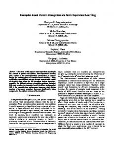
The contraction coefficient of the maps 1, . . ., A, is k 苸 (0,.]. In this study, we set k = .. The exact assignment i → ti of symbols i to vertices ti is not important, as long as the assignment is unique. Given an L-block u = u1u2 . . . uL 苸 AL, its spatial image, T(u) 苸 X, is found as follows: 1. Start in x0 = {.}D, the centre of the hypercube X. 2. Sliding through the L-block u left-to-right, for n = 1,2, . . ., L, iteratively move to xn = i(xn⫺1), provided the nth symbol un is i. 3. The image of the L-block u under the map T corresponds to the point we move to after observing the last symbol uL, i.e. T(u) = xL. As an example, consider an L-block u = . . . 142 over a four-symbol alphabet A = {1,2,3,4}, the last three symbols of which are 142. Let the four affine maps on the unit square X = [0,1]2, corresponding to the symbols in A, be defined as (k = .) 1(x) = .x + .(0,0), 2(x) = .x + .(1,0) 3(x) = .x + .(0,1), 4(x) = .x + .(1,1) Here, symbols 1, 2, 3 and 4, are associated with the unit square corners t1 = (0,0), t2 = (1,0), t3 = (0,1) and t4 = (1,1), respectively. Each map i(x), i = 1,2,3,4, first contracts the unit square [0,1]2 into the subsquare [0,.]2, and then shifts the subsquare towards the corresponding corner ti of the unit square. This is illustrated in Fig. 1. Imagine we have already processed the first L ⫺ 3 symbols u1u2 . . . uL⫺3 in the L-block u, so that, starting in x0 = (.,.), we ended up in a point xL⫺3 = T(u1u2 . . . uL⫺3) in the unit square X. Under

287

the map 1(x), the black unit square at the top left is contracted and then shifted, so that it fills the subsquare position associated with symbol 1. The shift vectors ti are schematically shown as the corresponding symbols i appearing at the corners of the unit square. The point xL⫺2 = T(u1u2 . . . uL⫺31) lies somewhere in the black subsquare at the corner marked by symbol 1. The whole process is iteratively repeated. The next symbol in u is 4. Again, the unit square is contracted into [0,.]2, but this time the contracted subsquare is shifted to the upper right corner of the unit square. Upon seeing the last symbol in u, 2, the result of the previous step is contracted into [0,.]2 and shifted to the lower right corner of the unit square. The points xL⫺1 = T(u1u2 . . . uL⫺314) and xL = T(u1u2 . . . uL⫺3142) lie inside the (increasingly shrinking) black subsquares in the corresponding plots. Note that by iteratively making contractions and shifts, we effectively code the history of recently seen symbols into subsquares of [0,1]2. Black subsquares inside unit squares in Fig. 1 correspond to seen strings schematically written on top of the squares. For example, the black square at the top left of Fig. 1 codes the state of total ignorance – every string over A could have been seen. The black subsquare inside the unit square labelled by *1 corresponds to all strings ending with symbol 1. The black ‘subsubsquare’ in the unit square labelled by *14 lies in the subsquare corresponding to strings ending with 4 (shaded area) and codes all strings ending with 14. Likewise, the black region in the unit square labelled by *142 corresponds to all strings ending with 142. Two properties of such IFS-driven spatial representations of symbolic sequences are of importance to us. First, if histories of the last symbols in two L-blocks u,v, are the same, i.e. if the strings u and v share a common suffix, their representations T(u) and T(v) lie close to each other. Secondly, the longer is the common suffix shared by u and v, the smaller is the region containing the points T(u) and T(v). For a rigorous treatment of fractal representations of symbolic sequences driven by iterative function systems [30]. We now describe predictive models that we call Fractal Classification Machines (FCM). These models are designed to efficiently use deep memory when inferring the next symbol. The inference is viewed as a classification task. The FCMs operate as follows: 1. Create a set D of training examples for a classifier operating on X by sliding a window of length L through the training sequence S = s1s2 . . . SN: (a) for each position p = 1,2, . . ., N–L, of the window, transform the L-block = spsp+1%sp+L−1 u = u1u2%uL = Sp+L−1 p

Fig. 1. Illustration of the iterative function system behind the spatial representation of symbolic streams. Each symbol 1, 2, 3 and 4 is associated with a unique corner of the black unit square at the top left. Upon seeing symbol 1, the unit square is contracted and shifted towards to corner associated with symbol 1. This process is iteratively repeated as more new symbols arrive. Increasingly longer sequences are coded in the shrinking copies of the original black unit square. In each construction step, the resulting unit square is labelled by the suffix coded by the black subsquare.

appearing in the window into the point T(u). (b) the set D contains all couples (T(u), s), such that u 苸 [S]L is an L-block in S, and s is the symbol following u in S. In other words, the set ), si+L)兩i = 1, 2, %, N − L} D = {(T(Si+L−1 i consists of labelled points T(u) that are spatial rep-

288

resentations of L-blocks u 苸 [S]L in S. The points are labelled with the corresponding next symbols in S. 2. Upon seeing a new history of L symbols, v = v1v2 . . . vL, 苸 AL, we make a guess about the next symbol by (a) mapping the L-block v into T(v), and (b) predicting the next symbol as the class label for T(v) returned by the K-Nearest-Neighbour (KNN) classifier [32] operating on the set D. The KNN classifier finds K points yi 苸 X, such that (yi, ␬i) 苸 D, i = 1,2, . . ., K, that are closest (in Euclidean distance) to T(v). Then, it consults the corresponding labels ␬1, ␬2, . . ., ␬K 苸 A. The class assigned to T(v) is the symbol appearing most often among the labels ␬1, ␬2, . . ., ␬K. The radius of the neighbourhood of T(v) in X involved in predicting the next symbol depends on the density of labelled points from D around T(v) and on the parameter K determining the number of labelled samples from D we wish to consult. For fixed K, the neighbourhoods around T(v) will be small in dense regions that correspond to Lblocks sharing a long common suffix. In other words, if the last L symbols v = v1v2 . . . vL happen to share a deep suffix with a subset of L-blocks seen in the training sequence, then our decision about the next symbol will be based upon that subset, which effectively amounts to a prediction with a deep memory. If, on the other hand, the region around T(v) is relatively sparse, then the effective memory involved in predicting the next symbol will be shorter. Also, the smaller is the parameter K, the smaller neighbourhoods around T(v) are considered, and hence the deeper is the memory used for prediction. In this sense, FCMs using relatively small values for the parameter12 K correspond to variable memory length Markov models with a preference for deeper memory. For a different variant of finite-memory fractal-based predictive models constructed by vector quantising the L-block representations in the set D [1,16,33].

P. Tin¯ o et al.

{Vt} calculated from the observed option prices by inverting the Black–Scholes formula (see the appendix). The basic trading strategy is to buy (sell) at-the-money straddles whenever volatility is predicted to increase (decrease). Since at-the-money straddles are approximately delta-neutral, there is no need to delta-hedge, and the strategy is thus a pure volatility trading strategy. In detail, every day, a constant amount of money is invested to buy (sell) the straddles, and on the next day, the straddles are sold (bought). If a model is uncertain about the sign of the volatility change (equal evidence for increase and decrease), the invested money is put into the bank at an annualised interest rate of 4%. The second data set contains intra-day bid-ask prices of (American-style) options on the FTSE 100 between 29 May 1991 and 29 December 1995 (which covers a period of 1161 trading days). The option prices are recorded synchronously with the FTSE 100 and time-stamped to the nearest second. Since our trading strategy is set up on a daily basis, we have to fix a reference point in time on each trading day. This reference point is 3 pm on normal trading days, and 12 pm on days where the stock exchange closes earlier. To trade straddles as in the DAX experiment, we extract the first quotes of call and put options with the same strike price that is as close as possible to the FTSE 100 at that time. For these options, which are roughly at-the-money, we calculate the average of bid and ask prices as a proxy of a reasonable option price. Then the prices of call and put options are added to obtain the straddle price. During this procedure, prices are carefully checked for outliers, recording errors, unusually large bid-ask spreads, and other sources of possible contamination. The final data set may thus be assumed to contain prices at which transactions could have been made at the market over the experimental time period. The series of returns rt of the financial indexes DAX and FTSE 100 obtained from daily index values xt via rt = logxt − logxt−1

(4)

are shown in Fig. 2.

4. DATA, VOLATILITY MEASURE AND TRADING STRATEGY We encourage readers not familiar with option contracts and option pricing to consult the appendix prior to reading this section. Our first data set consists of daily closing values of the DAX and daily closing prices of (European) call and put options on the DAX, from August 22 1991 until June 9 1998, which covers a period of 1700 trading days. In particular, the prices of the first in-the-money and the first outof-the-money call and put option are available.13 As a volatility measure, we chose the implied volatilities

12 13

In our experiments, K 苸 {3,5, . . ., 11}. The at-the-money point is assumed to be the closing value of the DAX.

5. EXPERIMENTAL SETUP Given the series {Vt} of estimated daily volatilities, we create a new series {Dt} of daily volatility differences Dt = Vt ⫺ Vt⫺1. On the basis of the series {Dt}, we construct, select and test predictive models used in our trading strategy. As mentioned in the introduction, to deal with nonstationarity in {Dt}, we use the sliding window technique. At each position, the sliding window of length 630 contains the training set (the first 500 points – roughly two years), followed by a validation set (125 point – roughly six months), and a test set (5 points – one week). Predictive models are estimated on the training set. Within each model class, the best performing candidate with respect to profit is selected on the validation set, and finally, the profit of the selected model is determined on the test set. Then the


Fig. 2. Series of daily returns of the financial indexes DAX and FTSE 100.

time window is shifted by five days, predictive models are re-estimated, etc. 5.1. Quantising Real-valued Time series into Symbolic Streams

再

1 (down), if Dt ⬍ 0 2 (up),

otherwise

(5)

Quantisation using four symbols is more involved, since we have to determine the positions of the cut values separating ‘normal’ from ‘extremal’ volatility differences Dt. The sequence {Rt} over the alphabet A = {1,2,3,4} is constructed as follows: for each position ␶ of the sliding window {Dt}␶␶⫹629: 1. We quantise the training set {Dt}␶␶⫹499 into the symbolic stream {Rt}T⫹499 , ␶

冦

1 (extreme down), if Dt ⬍ ␪1 ⬍ 0

Rt =

2 (normal down),

if ␪1 ⱕ Dt ⬍ 0

3 (normal up),

if 0 ⱕ Dt ⬍ ␪2

4 (extreme up),

if ␪2 ⱕ Dt

Q% of volatility decreases are considered extremal. The upper (100 ⫺ Q)% volatility decreases are viewed as normal. Analogically, Pˆ (·兩D ⱖ 0) captures the distribution of non-negative volatility differences in the training set. The upper Q% of volatility increases are considered extremal. The lower (100 ⫺ Q)% volatility increases are viewed as normal. In our experiments, we use the quantile values Q 苸 {10,20,30, . . ., 90}. 2. The validation symbolic sequence {Rt}␶␶⫹624 ⫹500 is obtained, for each Q 苸 {10,20,30, . . ., 90}, by quantising the realvalued validation set {Dt}␶␶⫹624 ⫹500 using the corresponding cut values ␪1, ␪2 determined on the training set. 3. For each predictive symbolic model, the optimal value Q* of Q 苸 {10,20,30, . . ., 90} is determined on the validation set: (a) both the training and validation sets are quantised using the same Q; (b) the model is fitted on the training set; (c) Q* is the value of Q which leads to the highest validation set profit. ␶⫹629 4. The test set {Dt}␶␶⫹629 ⫹625 is then quantised into {Rt}␶⫹625 using the cut values ␪1, ␪2 (determined on the training set) that correspond to the quantile Q*. 5.2. Predictive Models

Symbolic models operate on quantised versions of the realvalued series {Dt} of daily volatility differences. In particular, we perform quantisation into symbolic streams {Qt} and {Rt} over two and four symbols, respectively. The sequence {Qt} over the binary alphabet A = {1, 2} is obtained from {Dt} as follows: Qt =

289

(6)

The parameters ␪1 and ␪2 correspond to Q% and (100 ⫺ Q)% sample quantiles of the marginal empirical distributions Pˆ (·兩D ⬍ 0) and Pˆ (·兩D ⱖ 0), respectively, over the volatility differences D. The empirical distributions are calculated from the real-valued training set {Dt}␶␶⫹499. So Pˆ (·兩D ⬍ 0) describes the distribution of negative volatility differences in the training set, and the lower

To make predictions about the nature of the volatility move for the next day that will be used in our strategy for trading the straddles, we use the following predictive model classes: 쐌 MM(5) – Markov Models (MM) of order up to 5 (one week). This model class includes MMs of order 0,1,2, . . ., 5 (see Section 2). The model order for the test set is determined on the validation set. 쐌 MM(10) – MMs up to order 10 (two weeks). The class includes MMs of order 0,1,2, . . ., 10. As in the previous class, the model order is determined on the validation set. 쐌 PST(1) – Variable memory Length Markov Models (VLMM) with the associated Prediction Suffix Trees (PST) constructed using the ratio-related parameter scheme ⑀grow = ␳ 苸KL, ␳ = 1 (see Section 2). The case of ␳ = 1 is equivalent to the PST construction procedure introduced in Ron et al [15]. Maximum memory depth is set to L = 15 (three weeks). We build PSTs of various sizes by varying the threshold parameter ⑀KL as follows:14 ⑀KL 苸 {0.01, 0.005, 0.001, 0.0005, 0.0001, 0.00005, 0.00001}. The optimal value of ⑀KL is determined on the validation set. 쐌 PST(50) – regularised VLMMs with the associated PSTs constructed using the ratio coefficient ␳ = 50. All the remaining construction details are the same as in the class PST(1). 쐌 FCM – Fractal Classification Machines using deep memory in an efficient way (see Section 3). To test for 14 These parameter values were experimentally found to give a reasonable range of PST sizes.

290

P. Tin¯ o et al.

deeper memory structures, we set the maximum memory depth to L = 15 (three weeks). The parameter K can take on values K = 3,5, . . ., 11. The optimal number of nearest neighbours, K, is determined on the validation set. 쐌 NN – time-delay neural networks15 with a single linear output unit, three hidden units and inputs corresponding to the last 1, 3, 6 or 10 points from the training set. The transfer function of the hidden units is the standard 1⫺e⫺2x . The networks are tangent hyperbolic ␯(x) = 1⫹e⫺2x trained (using conjugate gradient) on the real-valued series {Dt} of daily volatility differences to predict the volatility difference for the next day. The optimal size of the network input is determined on the validation set. 쐌 NN-symb – time-delay neural networks with categorical output. The architectures of neural networks in this class are the same as those in the previous class NN, except for the output layer. Here, we have two output units with 1 . The the logistic sigmoid transfer function ␴(x) = 1⫹e⫺x output units correspond to the symbols 1 and 2 used in the two-symbol quantisation scheme. The networks are trained (again, using conjugate gradient) on the realvalued series {Dt} as input to predict the direction of the volatility move for the next day, i.e. 1 (decrease), or 2 (increase). 쐌 GARCH – GARCH(1,1) models [22] with a Gaussian distribution and a t-distribution. This model class was included as a benchmark, since it has been used in similar studies (e.g. [21,23]). In contrast to the previous model classes, the GARCH models are not trained on the precomputed series {Dt} of differences of historical volatilities. Instead, the GARCH models try to reconstruct the volatilities from the series of returns {rt} (Eq. (4)). Basic to these models is the notion that the series of returns {rt} can be decomposed into a predictable component ␮t and an unpredictable component et, which is assumed to be zero mean Gaussian (or t-distributed) noise of finite variance ␴2t : rt = ␮t⫹et. The models are thus characterised by time-varying conditional variances ␴2t , and are therefore well suited to explain volatility clusters typically present in the series of returns. The conditional mean is modeled as a linear function of the previous value: ␮t = art⫺1 ⫹ b. For the GARCH(1,1) model, the conditional variance ␴2t is given by

␴ = a0 + a e 2 t

2 1 t−1

+ a2␴

2 t−1

(7)

At each sliding window position, the GARCH(1,1) models with a Gaussian and a t-distribution are fit, in the maximum likelihood framework, to the series of returns corresponding to the training set. The optimal form of the noise distribution (Gaussian vs. t-distribution) is then determined on the validation set. The GARCH model makes a prediction

15

Time-delay neural networks can be considered as non-linear autoregressive filters.

about the direction of the volatility change based on the sign of ␴2t ⫺ ␴2t⫺1. Given historical data, the models predict the sign of the next volatility change as follows: 쐌 MMs and PSTs trained on sequences over – 2 symbols: predict decrease (increase) when the model predicts symbol 1 (2) with higher probability than symbol 2 (1); if the two probabilities coincide, output don’t know (equal evidence for decrease and increase) – 4 symbols: predict decrease (increase) when the sum of the predictive probabilities for symbols 1 and 2 (3 and 4) is greater than that for symbols 3 and 4 (1 and 2); if the two sums of probabilities coincide, declare don’t know. 쐌 FCMs on sequences over – 2 symbols: predict decrease (increase) when FCM classifies the spatial image T(v) of the recent history of symbols v as class 1 (2); FCMs cannot make a don’t know statement, since we use only odd values for the parameter K in the K-nearest neighbour classification – 4 symbols: predict decrease (increase) when, out of the K nearest neighbours of T(v), the number of points labelled with 1 or 2 (3 or 4) is greater than the number of points labelled by 3 or 4 (1 or 2).16 쐌 NNs predict decrease (increase) provided the output is negative (positive). Otherwise, declare don’t know. Since prior to training, the network weights are randomly initiated, we stabilise the network classification decisions by training a committee of 10 networks (for each input size – 1, 3, 6 and 10). Given an input, each member of the committee makes its prediction (decrease, increase, or don’t know). The overall output of the committee is then based on the majority vote. 쐌 NNs with categorical output (NN-symb) predict decrease (increase), when the activation of the output unit corresponding to symbol 1 (2) is greater than that of the other unit. If the activations are the same, declare don’t know. The committee technique described for the class NN is used also in this class. 5.3. Taking the Non-stationarity Seriously

At each position of the time-window, the models are fitted to data that start 2. years before their actual use for volatility predictions on the test set. This can be dangerous, especially when sudden large ‘stationarity breaks’ are present in the data (see Pesaran and Timmermann [34]). On the other hand, as discussed in the introduction, using a shorter sliding window can lead to undesirable overfitting effects. Our idea is to use yet another model class, Simple, that is a small collection of simple, fixed predictors requiring no

16 Note that in this case, FCM may predict an increase, even though the largest number of neighbors belong to, say, class 1. What is important are the summed class counts for down and extreme down (up and extreme up).


training on the training set. A suitable candidate model to be applied on the test set is selected on the validation set. The class Simple avoids using the training data since they form the oldest part in each sliding window. Of course, the price to pay is the fixed nature of the models in Simple. However, in financial prediction tasks, simple, short memory models often outperform more sophisticated predictors. Our choice of models for the class Simple is a collection of four simple-minded predictors operating on the series of volatility differences quantised using the two-symbol scheme: always predict 1 (decrease), always predict 2 (increase), copy the last symbol and reverse the last symbol (i.e. predict the other symbol). We hope to build a more powerful prediction strategy by combing the model classes M summarised in Section 5.2 with the class Simple. At each position of the time-window and for each model class M, we switch between the winner candidate of M and the winner from Simple in two ways: 1. Select between the two candidates based on the mean profit achieved on the validation set. We denote this technique by Comb-Val. This may not always work, since the consecutive validation sets are highly overlapping and a good validation set profit can be generated on an older part of the set, while the more recent profits can be negative. Similarly, a bad validation set performance may be caused by negative profits on an older part of the validation set, while the model performance on the more recent days may be quite good. What matters is the slope of average validation set profits corresponding to recent time-window positions. The slope tells us whether in the history of recent mean validation set profits there is a tendency towards improving the model performance, or not. Moreover, the magnitude of the slope reflects the strength of such a tendency. 2. Therefore, we compute the mean (per-day) validation set profits of the winner candidates from M over the last eight time-window positions (two months of test data). We do the same for the Simple model class. In both cases, we compute the slope in the recent history of eight mean validation set profits by regressing the last eight mean validation set profits using a linear regression. Note that if one of the more recent validation set profits is unusually high (e.g. due to some abrupt change in the market conditions), the linear regression will yield a steep slope, but the ‘outlier’ character of such a profit will be reflected in a broad confidence interval for the slope. Therefore, we determine the 95% confidence interval for the slopes and consider only the slope corresponding to the lower boundary of the confidence interval. If both slopes are positive, we select the candidate with the higher slope; if they are negative, we choose between the winner from M and Simple based in the current mean validation set profit (strategy Comb-Val). If the slopes are of different sign, use the candidate corresponding to the positive slope. We denote this method by Comb-LR.

291 5.4. Performance Measures

For each model class, we evaluate the overall test set profit by concatenating the test set profits for all time-window positions. All profits are expressed as the percentage of money we invest each day; 0 means no profit. A big advantage of this approach is that all results are scalable and readily interpretable for any amount of money we wish to invest. The first quantity we report is the mean of the series of concatenated test set profits, i.e. the mean profit per-day before transaction costs. Many studies in the literature on automatic trading report standard deviations and t-test-related significance results for the series of daily profits. There are two difficulties with such reports: 1. The unconditional distribution of daily profits is usually far from Gaussian. In particular, it is fat-tailed, i.e. it has excess kurtosis. In this case, the application of t-tests is not justified. On the other hand, using standard nonparametric tests based on ordering the joint series, like the Wilcoxon or Mann and Whitney U-tests [35], may not be economically meaningful. Consider comparing two series of profits that are equal up to the last profit, which is 0 in the first series and a very large loss of money in the second series. The non-parametric test would still claim that the two series are not significantly different. 2. Standard deviations computed from the series of daily profits provide an estimate of the risk involved in investing your money, if you wanted to trade just for one day. This is not what a reasonable trader would do. He or she may be interested in assessing the risk involved in trading for some fixed, longer period of time. Therefore, we partition the time series of daily profits into non-overlapping blocks of length ᐉ, and compute a new series of average daily profits achieved within each block. Since the daily test set profits are virtually uncorrelated,17 if the block length ᐉ is long enough, by the central limit theorem, the average block-profits18 are approximately Gaussian-distributed.19 Hence we can subject the series of average block-profits to t- and paired t-tests. The significance level for both tests is set to 95%. The standard deviation computed from the series of average block-profits estimates the risk involved in trading over a period of ᐉ days. The mean remains unchanged, since the average of the average block-profits is the average profit per-day. There is an upper bound on the block length ᐉ, too. Large ᐉ means smaller number of blocks in the partition of the daily profits, and hence smaller number of average block-profits for computation of the standard deviation and significance tests. Considering the lengths of the series of daily profits in the

17

At the 95% confidence level. The average profits per-day computed within the blocks. 19 The central limit theorem is formulated under asymptotical considerations: when the number of i.i.d. random variables approaches infinity, the distribution of their average is Gaussian. However, the distributions of the averages approach the Gaussian distribution very fast, as the number of variables increases (40 random variables are usually sufficient). 18

292

P. Tin¯ o et al.

DAX and FTSE experiments, we set the block length ᐉ to 60 (3 months) and 40 (2 months), respectively. To account for Transaction Costs (TC), we report the maximum amount20 that we can subtract from each daily profit, so that the average block-profits still have a significantly positive mean (under the t-test).

into a single profit series. This series is then partitioned into several non-overlapping blocks of constant length. For each block we compute the average profit per-day. Finally, we report various statistics computed on thus obtained series of average block-profits.

5.5. Summary of the Experimental Setup

6. RESULTS AND DISCUSSION

The overall picture of our experimental setup is shown in Fig. 3. A sliding window contains a training, a validation and a test sequence. Sequences of daily volatility differences appear in the sliding window in the (original) real-valued form, or as symbolic streams produced in the quantisation step. At each sliding window position, and for each model class M, the models from M are trained on the training sequence. Then the models are used to predict the signs of volatility differences on the validation set. These predictions are used as trading signals in our trading strategy, thereby producing a series of validation set profits. Based on the average validation set profit, we select the candidate of the model class M to be used on the test set.21 The selected candidate is then used to predict the signs of volatility differences on the test set, which are in turn plugged into the trading strategy to produce the test set profits. Also, at each position of the sliding window and for each model class M, we save the average profit achieved on the validation set by the selected candidate from M. The series of average validation set profits are used in methods Comb-Val and Comb-LR that combine simple strategies from Simple with the more complex model classes studied in this paper. After the sliding window reaches its final position, for each model class, we concatenate all the daily test set profits

Tables 1–3 present results for both the DAX and FTSE 100 experiments. The performances of symbolic models operating on the binary sequences and sequences over the four-symbol alphabet are shown in Tables 1 and 2, respectively. The results of the models operating on the real-valued sequences are reported in Table 3. Shown are the average profits perday (before transaction costs) achieved by the base model classes and the two associated combination strategies importing simple methods into the more sophisticated base model classes (see Section 5.3). Standard deviations reflect the variations among the average block-profits. Furthermore, we show significance results obtained by running paired t-tests on the average block-profits. In particular, we compare each predictor with the class Simple, and we also compare the combined strategies (switching between the base model class and Simple) with the base model class: (⫺) means that the model class performance is significantly worse than that of Simple, (⫹) appears where a combined strategy significantly outperforms the base model class, (*) indicates that the realised profit is significantly higher than the profit of the simple strategy. Finally, we report the highest Transaction Costs (TC) that can be taken out from daily profits, so that the average block-profits still have a significantly positive mean (under the t-test). To test the usefulness of our notion of volatility for automatic trading strategies, we report profits for the hypothetic Always Correct Predictor (ACP), i.e. the predictor that always knows in advance the sign of the next volatility difference. Several observations can be made based on the experimental results:

Fig. 3. An illustration of the experimental setup used in the DAX and FTSE 100 experiments.

20

Expressed, as in the case of daily profits, as the percentage of money we invest every day. 21 When quantisation into four symbols is used to pre-process the data, the optimal quantisation quantile is also determined on the validation set.

1. The profits gained by the hypothetic Always Correct Predictor (ACP in Table 1) show that, theoretically, predicting daily volatility changes (with volatilities estimated by implied volatilities) provides a good basis for automatic trading strategies buying/selling straddles. We also tried another popular measure of volatility – the average of the past squared returns with exponentially declining weights – also known as RiskMetrics [36,37]. Such volatility measures were advocated as being wellsuited for the purpose of trading options on financial indexes by Figlewski [38] (see also Schmitt and Kaehler [39]). Interestingly enough, compared with implied volatilities, we got almost the same (DAX experiment) or less favourable (FTSE 100 experiment) results when using the RiskMetrics notion of volatility. 2. In general, profits generated by automatic trading of straddles are higher in the FTSE 100 experiment than


3.

4.

5.

6.

in the DAX experiment (see Tables 1, 2 and 3), suggesting that the option market for the DAX seems to be more efficient than that for the FTSE 100. As typical in financial prediction tasks, simple-minded predictors in the class Simple are difficult to beat by more complicated models, and should definitely be considered in studies like this one. In general, the binary quantisation scheme leads to better results than the more refined four-symbol scheme (see Tables 1 and 2). This is primarily due to the short lengths of the training sequences – a burden typical of daily financial data. We are highly sceptical about using more than four symbols in the quantisation scheme. In applications like this one, we advise to start with two symbols, and if desired, carefully and in a controlled way, add further quantisation levels. On average, the binary Markov Models (MMs) (see the rows corresponding to MMs in Table 1) outperform the continuous-valued neural networks and GARCH models (Table 3). This confirms, in a realistic trading setting, the previous findings [2,3,7–10,33] that quantising realvalued time series in the financial domain may be beneficial. Comparing ‘pure’ model performances without combing

293

with the class Simple, the highest per-day profits are obtained by the binary Markov Models (MMs) with memory depth up to one week (class MM(5)). Higher order MMs (from the class MM(10)) are prone to overfitting (each of our training sets contained only 500 items). 7. Apart from the 4-symbol scheme in the DAX experiment, Prediction Suffix Trees (PST) do not outperform the fixed-order MMs (see Tables 1 and 2). This illustrates the phenomenon we addressed earlier [1,16], that there are many practical problems in fitting Variable memory Length Markov Models (VLMM). One-parameter construction schemes, like that presented in Ron et al [15] and used here (see Section 2), operate only on small subsets of potential VLMMs. Especially when trained on relatively short sequences generated by processes with a rather shallow memory, VLMMs tend to overestimate the data structure. Even the regularisation procedure using ⑀grow = 50⑀KL (see Section 2), which we found useful in other contexts [16], did not improve the VLMM profits. Simply stated, VLMMs are ‘too sophisticated’ for financial forecasts of the kind studied in this paper. 8. Neural networks tend to overestimate the structure in the training data. Forcing them to predict only the

Table 1. Profits of the symbolic models operating on the binary sequences in the DAX and FTSE 100 experiments. Combined strategies are referred to by the employed selection method. Combined strategies using simply the validation set performances and those using the slopes of linear regression on the past validation set performances are referred to as Comb-Val and CombLR, respectively. For comparison, we also report profits that would be made by the Always-Correct-Predictor, ACP, perfectly predicting all the volatility changes. To make a more realistic assessment of the achieved profits, we also report the maximal Transaction Costs (TC) that one can subtract from each daily profit, so that when subjected to the t-test (p = 0.05), the average block-profits are still significantly positive Model class

DAX % profit per-day Mean

FTSE 100 Highest TC for signif. pos. mean

Std.

% profit per-day Mean

Std.

Highest TC for signif. pos. mean

ACP

1.310

0.652

1.034

2.706

1.109

2.132

Simple

0.423

0.521

0.21

1.676

1.222

1.05

MM (5) Comb-LR Comb-Val

0.262 0.497 0.430

0.603 0.485 0.458

0.01 0.30 0.24

1.551 1.611 1.551

0.833 0.884 0.833

1.12 1.16 1.12


0.208 0.473 0.425

0.668 0.613 0.578

– 0.22 0.19

1.490 1.550 1.489

0.894 0.942 0.894

1.03 1.07 1.03

PST (1) Comb-LR Comb-Val

0.013⫺ 0.307⫺ 0.449⫹

0.584 0.535 0.509

– 0.08 0.23

0.703⫺ 1.604⫹ 1.640⫹

1.312 1.235 1.195

0.03 0.97 1.03

PST (50) Comb-LR Comb-Val

⫺0.013⫺ 0.394⫹ 0.421⫹

0.568 0.479 0.509

– 0.19 0.20

1.493 1.405 1.485

0.878 0.826 0.876

1.04 0.98 1.04

FCM Comb-LR Comb-Val

⫺0.243⫺ 0.371⫹ 0.471⫹

0.451 0.417 0.404

– 0.19 0.30

0.568⫺ 1.644⫹ 1.538⫹

0.918 0.642 1.055

0.10 1.30 1.00

294

P. Tin¯ o et al.

Table 2. Profits and affordable Transaction Costs (TC) of the symbolic models operating on the sequences over the foursymbol alphabet in the DAX and FTSE 100 experiments (implied volatility) Model class



Std.

% profit per-day Mean

Std.



0.043⫺ 0.335 0.311

0.679 0.604 0.592

– 0.08 0.07

1.381 0.959⫺ 1.381

1.357 1.094 1.357

0.68 0.40 0.68

PST(1) Comb-LR Comb-Val

0.172 0.507 0.537

0.671 0.528 0.583

– 0.28 0.29

0.541⫺ 0.967⫺ 1.138⫺

0.592 0.903 1.126

0.24 0.50 0.56

PST(50) Comb-LR Comb-Val

⫺0.008⫺ 0.275⫺ 0.307⫺

0.736 0.597 0.616

– 0.02 0.04

1.012⫺ 1.122 1.044

0.958 1.135 0.944

0.52 0.54 0.56

FCM Comb-LR Comb-Val

⫺0.205⫺ 0.351⫹ 0.414⫹

0.490 0.499 0.514

– 0.14 0.19

0.385⫺ 1.038⫺ ⫹ 1.125⫺ ⫹

1.233 1.013 0.942

– 0.52 0.64

Table 3. Profits and affordable Transaction Costs (TC) of the models operating on the real-valued sequences in the DAX and FTSE 100 experiments (implied volatility) Model class


Std.

NN Comb-LR Comb-Val

0.0326⫺ 0.397 0.405⫹

0.576 0.599 0.554

NN-symb Comb-LR Comb-Val

0.123 0.410 0.375

GARCH Comb-LR Comb-Val

0.079(⫺) 0.408 0.437(⫹)


% profit per-day


Mean

Std.

– 0.15 0.18

1.331 1.562 1.432

1.095 1.121 1.131

0.77 0.99 0.85

0.773 0.574 0.550

– 0.17 0.15

1.541 1.470 1.429

0.777 0.973 1.033

1.14 0.97 0.90

0.420 0.671 0.684

– 0.13 0.15

0.092 0.116 0.175

1.394 1.056 1.123

– – –

principal trends (increase/decrease) in the series of daily volatility differences leads to better profits (compare entries in Table 3 corresponding to NN and NN-symb). However, detailed values of volatility differences presented at networks’ inputs are not necessary, and can actually be misleading. Our results indicate that nothing is lost by using simple Markov models fed by the quantised inputs (MM(5) entry in Table 1). 9. In most cases, the combination strategies Comb-LR and Comb-Val work well, increasing the mean and/or decreasing the variance of the block profits. Sometimes, a combination of the base model class with the Simple class

achieves better results than those achieved by the two model classes themselves (e.g. Comb-LR technique using binary Markov models in the DAX experiment, see Table 1). As an illustration, we show in Fig. 4 cumulative profits (expressed in percentage of invested money) in the DAX experiment, achieved by the class MM(10) of Markov models up to order 10, the class Simple, and the combination Comb-LR of MM(10) and Simple. In general, none of the combination methods Comb-LR, Comb-Val, seems to outperform the other one. 10. By their nature, Fractal Classification Machines (FCMs) are forced to use deep memory. Maximum memory depth


Fig. 4. Cumulative profits gained by the class MM(10) of Markov models of maximal order 10, the class Simple, and the combination Comb-LR of MM(10) and Simple in the DAX experiment. The profits are expressed in percentage of invested money.

is set to 15, which would be inconceivable with classical Markov Models (MMs), given the short length of the training sequences. Inevitably, FCMs suffer more from overfitting than MMs, where for each sliding window position, the order can be selected between 0 and 5 (10), depending on the validation set performance. PSTs are also constructed with maximum memory depth 15, but the individual prediction trees can be very shallow, depending on the construction parameters’ values. We used FCMs to test how good the combination strategies are in switching between the long-memory FCM predictions and the short-memory predictions of Simple. In the DAX and FTSE 100 experiments, under the binary quantisation scheme, the combination schemes Comb-Val and Comb-LR, respectively, work very well (see the Comb-Val and Comb-LR FCM entries in Table 1 for DAX and FTSE 100 experiments, respectively). This indicates that a profitable series of volatility predictions can be obtained by switching between the two extremes, i.e. long-memory and shortmemory regimes. In combination with Simple, FCMs can be very powerful. Hence, to make profitable volatility predictions, we do not have to use models with a wide spectrum of memory depths. It is sufficient to switch between shallow memory models (such as those in the class Simple) and models like FCMs that use deep memory in an efficient way. 11. It may be interesting to analyse the data by plotting and comparing characteristics of the selected candidates from the predictive model classes used in the technical trading. For example, in Fig. 5 corresponding to the DAX experiment, we show the evolution of memory depths in the classes MM(5) and MM(10) of binary Markov models of maximal order 5 and 10, respectively (upper graph). For each trading day, we show the order

295

of the Markov model that was selected on the corresponding validation set as the candidate from the class MM(5) (MM(10)).22 Models from the class MM(10) tend to use either a shallow (order 0–1) or a rather deep (order 8–10) memory. Very few intermediate memory lengths are used. Note the sharp changes from lowor no-memory regimes to deep memory contexts in the plot for the model class MM(10). The history of active strategies from the class Simple (always predict Up (U), always predict Down (D), copy the last symbol (C) and reverse the last symbol (R)) is shown in the lower graph of Fig. 5. For each trading day, the active strategy was selected based on the validation set performance. Note that there seems to be a correlation between memory depths selected in the class MM(5) and strategies picked up from the class Simple. Roughly, in periods dominated by MM orders 1 and higher (days 1–70 and 700–970), strategies always predict Up and reverse the last symbol are selected. In periods dominated by memoryless MMs23 (order 0), the strategies always predict Down and copy the last symbol seem to be preferred. Such an analysis is beyond the scope of this paper, but it is an interesting direction for future research. 12. Schmitt and Kaehler24 [39] distinguish three groups of investors: market makers, other registered traders (traders) and non-members of the exchange, with transaction costs25 per straddle of 0.1%, 0.5% and 1%, respectively. To be on the safe side, we double the transaction costs, i.e. we assume that market makers, traders and non-members pay 0.2%, 1% and 2%, respectively, of their profit as transaction costs. The experimental profits suggest that the option market for the DAX is not efficient from the point of view of market makers, but it is efficient from the standpoint of registered traders and non-members. The option market for the FTSE 100 seems to provide the market makers and registered traders with an opportunity to generate (in an automatic way) an excess profit. The market is efficient for non-members of the exchange. We stress that we provide a rather pessimistic assessment of profits. Consider the following example: we buy a straddle on day t; according to our strategy we will sell it the next day; but on day t ⫹ 1 we may decide to buy the same straddle again. In this case, it would be better to keep the straddle until we decide, based on the volatility prediction, to sell it.

22 The MM order determines how far into the past the model looks in order to predict the nature of the next volatility move. MM of order 0 simply predicts the most frequent symbol in the training set. MM of order 1 looks back one day and based on the nature of the most recent volatility change determines the next volatility move. The predictive probabilities (conditional on what happened in the previous day) are calculated on the training set. MM of order 2 considers the last 2 volatility changes, etc. 23 MMs that just count the numbers of Ups and Downs in the training set. 24 Schmitt and Kaehler traded straddles on the DAX index at the German Futures and Options Exchange (Deutsche Terminbo¨ rse – DTB). The transaction cost estimates reported [39] and used here are based on the information provided by DTB. We assume similar transaction costs for trading straddles on the FTSE 100 at LIFFE.

296

P. Tin¯ o et al.

Fig. 5. Characteristics of representatives of the binary model classes MM(5), MM(10), and Simple in the DAX experiment. For trading day we plot the MM order (upper graph), and the selected strategy from Simple (lower graph). The strategies always Up, always Down, reverse last, copy last are denoted by U, D, R and C, respectively.

This way we could avoid having to pay the transaction costs every day. Also, traders like us, that trade on a daily basis and are willing to invest potentially large amounts of money,26 usually negotiate at the stock exchange a special discount rate for the transaction costs. 13. It may seem, as suggested by one of the anonymous reviewers, that the length of the test period for each time-window position (five days) is too short and may result in unstable overall trading results. However, the stability of the results is not lost because the training sets in neighbouring time-window positions are highly overlapping. This means that there will be little difference between deterministically constructed models (classes MM, PST, FCM) built in neighbouring time-window positions. There is a potential for instability in the class NN, since the neural networks are randomly initiated, but the model construction instability is decreased by using committees of networks as opposed to predicting with a single neural network. 26

The actual invested amount of money is not specified in the experiments, since we report our profits as a percentage of the invested money.

To support our arguments, we run a new set of experiments with time-windows containing test sets of length 20 (1 month) and 40 (2 months). Note that by prolonging the test period, the number of experimental time-window positions is reduced (see Fig. 3). The predictive model classes considered in the new experiments were the Markov Models (MM) and Neural Networks (NN). Compared with our original (5-day-test-set) experiments, standard deviations of the block-profits are roughly the same. In fact, they are slightly higher in the DAX experiment (0.6–0.8) and in a wider range in the FTSE 100 experiment (0.6–1.2). In the DAX experiment, the mean profits significantly decreased with increasing test set length. This pulled the highest affordable Transaction Costs (TC) to the negative range, even for the compound models using the class Simple. In the FTSE 100 experiment, the mean profits were in the same range as in our original experiments.

7. CONCLUSION We considered a realistic trading setting, where straddles are traded based on predictions of differences of daily vola-


tilities of the underlying. When dealing with daily financial time series, typically, one has to cope with relatively short training sets. In two independent and controlled experiments, we showed that in such cases, quantisation of realvalued sequences can help to analyse patterns underlying the evolution of the system, which could otherwise be masked by large amounts of noise and/or few dominant outliers. We proposed a data-driven parametric quantisation scheme. Using fewer symbols (quantisation levels) is preferable. In general, symbolic Markov Models (MMs) were able to achieve larger profits than the models operating on realvalued sequences. The model order of MMs was selected on an independent validation set. To deal with non-stationarity in the daily data, we used the sliding window technique and proposed to add a special class of fixed, simple symbolic predictive models. Such models avoid using older, and potentially misleading parts of the sliding window devoted to the training data. We presented two techniques for incorporating these simple predictors into more sophisticated models that are fitted on the training set. This approach proved to be of great benefit for most of the studied model classes. We also studied the memory structure in the time series of daily volatility differences using a novel variation on our own fractal-based symbolic predictive models introduced earlier [1,16]. Such models use deep memory in an efficient way. Two memory regimes, characterised by deep and shallow memory, seem to dominate the studied financial time series. Our experiments show that market makers involved in trading options on the DAX and the FTSE 100 can generate, in an automatic way, an excess profit. However, for nonmembers of the exchange, the option markets on the DAX and the FTSE 100 are efficient. The option market for the DAX seems more efficient than that for the FTSE 100. Except for the GARCH models, the predictive model classes used in this paper have a bounded (although potentially long) memory. We are currently investigating the trading potential of models with theoretically unbounded memory, such as recurrent neural networks. Acknowledgements

This work was supported by the Austrian Science Fund (FWF) within the research project ‘Adaptive Information Systems and Modeling in Economics and Management Science’ (SFB 010). The Austrian Research Institute for Artificial Intelligence is supported by the Austrian Federal Ministry of Science and Transport. Many thanks go to R. Tompkins for valuable discussions on trading options and for suggesting a regime-shifting model for predicting the daily volatility differences. We are thankful to the anonymous reviewers for many useful suggestions that helped to improve the paper presentation.

References 1. Tin˘ o P, Dorffner G. Building predictive models from fractal representations of symbolic sequences. Advances in Neural Information Processing Systems 12, MIT Press, 2000; 645–651

297 2. Giles CL, Lawrence S, Tsoi AC. Rule inference for financial prediction using recurrent neural networks. Proceedings of the conference on Computational Intelligence for Financial Engineering, New York City, NY, 1997; 253–259 3. Giles CL, Lawrence S, Tsoi AC. Noisy time series prediction using a recurrent neural network and grammatical inference. Machine Learning, 2001; 44: 161–183 4. Crutchfield JP, Young C, Computation at the onset of chaos. In: Zurek WH (ed) Complexity, Entropy, and the physics of Information, SFI Studies in the Sciences of Complexity, vol 8, Addison-Wesley, 1990; 223–269 5. Katok A, Hasselblatt B. Introduction to the Modern Theory of Dynamical Systems. Cambridge University Press, 1995 6. Buhlmann P, Wyner AJ. Variable length Markov chains. Annals of Statistics 1999; 27: 480–513 7. Papageorgiou CP. High frequency time series analysis and prediction using markov models. Proceedings of the Conference on Computational Intelligence for Financial Engineering, New York City, NY, 1997; 182–185 8. Papageorgiou CP. Mixed memory markov models for time series analysis. Proceedings of the conference on Computational Intelligence for Financial Engineering, New York City, NY, 1998; 165–170 9. Apte C, Hong SJ. Predicting equity returns from securities data. In: Fayyad UM, Piatetsky-Shapiro G, Smyth P, Uthurusamy R (eds), Advances in Knowledge Discovery and Data Mining, AAAI/MIT Press, 1994; 541–560 10. Buhlmann P. Extreme events from return-volume process: a discretization approach for complexity reduction. Applied Financial Economics 1998; (8): 267–278 11. Saul LK, Jordan MI. Mixed memory Markov models. Proceedings 6th International Workshop on Artificial Intelligence and Statistics, Fort Lauderdale, FL, 1998 12. Kohonen T. The self-organizing map. Proceedings of the IEEE 1990; 78(9): 1464–1479 13. Kohavi R, Sahami M. Error-based and entropy-based discretization of continuous features. In: Simondis E, Han J, Fayyad U (eds), Proceedings of the Second International Conference on Knowledge Discovery in Databases, AAAI Press, 1996; 114–119 14. Bengio Y, Simard P, Frasconi P. Learning long-term dependencies with gradient descent is difficult. IEEE Trans Neural Networks 1994; 5(2): 157–166 15. Ron P, Singer Y, Tishby N. The power of amnesia. Advances in Neural Information Processing Systems 6, Morgan Kaufmann, 1994; 176–183 16. Tin˘ o P, Dorffner G. Predicting the future of discrete sequences from fractal representations of the past. Machine Learning 2001 17. Singh S. A long memory pattern modeling and recognition system for financial forecasting. Pattern Analysis and Applications 1999; 2(3): 264–273 18. Singh S. Pattern modeling in time-series forecasting. Cybernetics and Systems – An International Journal 2000; 31(1): 49–66 19. van Biljon D. Predicting stock market prices with hidden markov models. MS thesis, Department of Computer Science, University of Stellenbosch, Stellenbosch, South Africa, 1999 20. Gregoir S, Lenglart F. Measuring the probability of a business cycle turning point by using a multivariate qualitative hidden markov model. Technical Report DP 9848, Economics Research Library, University of Minnesota, 1988 21. Noh J, Engle RF, Kane A. Forecasting volatility and option prices of the s&p 500 index. Journal of Derivatives 1994; (3): 17–30 22. Bollerslev T. A generalized autoregressive conditional heteroscedasticity. Journal of Econometrics 1986; 31: 307–327 23. Dockner EJ, Strobl G, Lessing A. Volatility forecasts and the profitability of option trading strategies. Technical Report, University of Vienna, Austria, 1988

298 24. White H. Economic prediction using neural networks: the case of IBM daily stock returns. Proceedings 2nd Annual IEEE Conference on Neural Networks II, 1988; 451–458 25. LeBaron B. Technical trading rule profitability and foreign exchange intervention. Journal of International Economics 1999; 49: 125–143 26. Guyon I, Pereira F. Design of a linguistic postprocessor using variable memory length markov models. International Conference on Document Analysis and Recognition, Monreal, Canada, IEEE Press, 1995; 454–457 27. Ron D, Singer Y, Tishby N. The power of amnesia. Machine Learning 1996; 25: 117–150 28. Weinberger MJ, Rissanen JJ, Feder M. A universal finite memory source. IEEE Trans Information Theory 1995; 41(3): 643–652 29. Rissanen J. A universal data compression system. IEEE Trans Information Theory 1983; 29(5): 656–664 30. Tin˘ o P. Spatial representation of symbolic sequences through iterative function system. IEEE Systems, Man and Cybernetics, A: Systems and Humans 1999; 29(4): 386–392 31. Barnsley MF. Fractals Everywhere. Academic Press, New York, 1988 32. Duda RO, Hart PE. Pattern Classification and Scene Analysis. Wiley, New York, NY, 1973 33. Tin˘ o P, Schittenkopf C, Dorffner G, Dockner EJ. A symbolic dynamics approach to volatility prediction. In: Abu-Mostafa YS, LeBaron B, Lo AW, Weigend AS (eds), Computational Finance, MIT Press, Cambridge, MA, 2000; 137–151 34. Pesaran MH, Timmermann A. Model instability and choice of observation window. Technical Report 99–19, Cambridge University, Cambridge, UK, 1999 35. Mann HB, Whitney DR. On a test of whether one of two random variables is stochastically larger than the other. Annals Mathematical Statistics 1047; 18 36. Morgan Guaranty Trust. RiskMetrics – Technical Document, Morgan Guaranty Trust Company Global Research, New York, 3rd ed, 1995 37. Boudoukh J, Richardson M, Whitelaw RF. Investigation of a class of volatility estimators. Journal of Derivatives 1997; 1: 63–71 38. Figlewski S. Forecasting volatility. Financial Markets, Institutions & Instruments 1997; 6(1): 1–88 39. Schmitt C, Kaehler J. Delta-neutral volatility trading with intraday prices: an application to options on the Dax. Technical Report No. 96–25, Zentrum fu¨ r Europa¨ ische Wirtschaftsforschung, 1996 40. Black F, Scholes M. The pricing of options and corporate liabilities. Journal of Political Economy 1973; 81: 637–654 41. Tompkins R. Options Explained. Macmillan, 1994

Appendix A: option pricing A holder of a European call option on an underlying asset S (e.g. a stock) has the right, but not the obligation, to buy the underlying (asset) at a specified price K (the strike price) at a specified time T in the future (at maturity). The strike price K and the maturity time T of the option are fixed when the option contract is signed at time t ⱕ T. If the price ST of the underlying at the maturity time T is larger than the agreed strike price K, the option holder will exercise his right to buy the underlying, thereby realizing a profit of ST ⫺ K ⬍ 0. If ST ⬍ K, his option is worthless. Therefore, the option payoff at the maturity time T is given by max {ST ⫺ K, 0}.

P. Tin¯ o et al.

The fair price C of a call option depends on the assumptions about the stochastic process driving the price St of the underlying asset S until maturity, i.e. for t ⱕ T. Black and Scholes [40] pioneered the field of option pricing by deriving a closed-form expression for the fair price C of a European call option. They assumed that the price process St of the underlying asset S follows a geometric Brownian motion with volatility ␴. Although real market dynamics are much more complicated, their famous formula

冉

冑

冊

C = StN(d1) − Ke−r(T−t)N d1 − ␴ T − t

d1 = N(d) =

冉冊

␴2 St ln + r + (T − t) K 2

冕

␴ 冑T − t

d

−⬁

1

冑 2␲

(8)

(9)

x2

e− 2 dx

(10)

where r denotes the riskless interest rate, is still applied by many traders at financial markets around the world. All variables in the Black–Scholes formula are explicitly known except for the volatility ␴ which must be estimated from the market data. A European put option gives the option holder the right to sell the underlying asset S at maturity time T for a specified (strike) price K, thereby yielding a profit max {K ⫺ ST, 0}. The option is thus worthless if the asset price at maturity, ST, is higher than the strike price K. In the Black– Scholes world, the fair price P of a put option is given by P = C + Ke−r(T−t) − St

(11)

where C is the price of the call option with the same strike price K and the same maturity time T. Depending on the value St of the underlying asset S at time t ⬍ T and the agreed strike price K, a call option is called in-the-money and out-of-the-money, if St ⬎ K and St ⬍ K, respectively. A put option is called in-the-money and out-of-the-money, if St ⬍ K and St ⬎ K, respectively. An option is called at-the-money, if St = K. A combination of a call option and a put option with the same strike price K and maturity time T is called a straddle on the underlying asset S, and its price is given by S = C ⫹ P. If a straddle is at-the-money, which roughly means that St = K, it is delta-neutral, i.e. small price changes ⌬St of the underlying asset S have a negligible effect on the straddle price S. In other words, the owner of the straddle is not exposed to market risk (with respect to price fluctuations). However, the straddle price does depend on changes in the volatility ␴ in prices St of the underlying asset S (the larger ␴, the larger S). Indeed, the sensitivity of straddle prices with respect to volatility ␴ is maximal for at-the-money straddles. Therefore, buying (selling) at-the-money straddles if volatility is expected to increase (decrease), is a volatility trading strategy which is mainly independent of the direction of price changes (see Tompkins [41] for more details). One of the popular approaches to estimating the


(inherently unobservable) volatility ␴ from historical data of the underlying asset prices St is to keep track of the prices of options on the underlying asset S that appeared in the past, and then invert an option pricing model (such as the Black–Scholes model given by Eqs (8)–(10)) to calculate the volatility parameter ␴. Volatility estimated in this manner is known as implied volatility. The volatility measure used in this study is the implied volatility estimated by inversion of the Black–Scholes model. In the Black– Scholes world, the volatility ␴ is assumed to be constant, and therefore one should obtain the same value of the implied volatility for options with different strike prices. In reality, however, volatility is not constant but often has the shape of a ‘smile’, if plotted against the strike prices. One way to deal with this inconsistency is to average the implied volatilities over a range of strike prices. For the DAX, the average value of the implied volatilities of the first in-themoney and the first out-of-the money call and put option is calculated. For the FTSE 100, the average value of the implied volatilities of the call and put option closest to the at-the-money point is used. So the average value of 4 (2) implied volatilities is calculated for the DAX (FTSE 100) every day. The definition of an American option is similar to the definition of a European option. The only difference is that the owner has the right to exercise his option whenever he or she wants, i.e. he or she can exercise the option before maturity time T. The pricing of American options is more

299

difficult, but one can use the prices of the corresponding European options as a rough approximation.

Peter Tin˘ o studied at Slovak Technical University (STU) and obtained his PhD (1997) from Slovak Academy of Sciences. He taught at STU and worked at the NEC Research Institute in Princeton NJ, USA and the Austrian Research Institute for AI in Vienna, Austria. He is currently a research fellow with the Neural Computation Research Group at Aston University, UK. His scientific interests are in visualisation, probabilistic modelling of static and dynamic data and dynamical systems.

Christian Schittenkopf studied at University of Innsbruck, Austria, and Technical University of Munich, Germany. He worked on his PhD (1997) at Siemens AG, Corporate Technology in Munich. Since 1998 he has been involved with the Austrian Research Institute for AI in Vienna, Austria. His research interests are in neural networks, probabilistic modelling of financial data and option pricing.

Georg Dorffner studied at Vienna University of Technology, Austria, and Indiana University, USA. He obtained his PhD (1989) from Indiana University. At present he is associate professor at the Department of Medical Cybernetics and AI, University of Vienna, and heads the Neural Networks Group at the Austrian Research Institute for AI in Vienna. His research interests are in neural networks, time series analysis and economic modelling, signal processing and connectionist models of conceptual development and language.

Correspondence and offprint requests to: P. Tin˘ o, Neural Computing Research Group, Aston University, Aston Triangle, Birmingham B4 7ET, UK. Email: p.tino얀aston.ac.uk

Volatility Trading via Temporal Pattern Recognition in ... - Springer Link

Volatility Trading via Temporal Pattern Recognition in ... - Springer Link

Suggest Documents

Serial-pattern structure and temporal-order recognition - Springer Link

Towards Spatio-Temporal Pattern Recognition Using ... - Springer Link

Quantum Pattern Recognition - Springer Link

Quantitative determination and pattern recognition ... - Springer Link

Volatility Trading

Temporal and spatial pattern of infant mortality in ... - Springer Link

Spatio-temporal pattern of viral meningitis in Michigan ... - Springer Link

Spatio-temporal pattern changes of land space in ... - Springer Link

Progress in Pattern Recognition, Image Analysis ... - Springer Link

Application of pattern recognition in arson investigation - Springer Link

Invariant Recognition of Spatio-Temporal Patterns in ... - Springer Link

Volatility in Returns from Trading

Review Spam Detection via Temporal Pattern Discovery

Video Segmentation via Temporal Pattern Classification - FXPAL

Vascular Pattern Localization via Temporal Signature

Video Segmentation via Temporal Pattern Classification - UFSM

Exemplar-based Pattern Recognition via Semi ... - CiteSeerX

Pattern Recognition Via Vasconcelos' Genetic ... - Semantic Scholar

The Intraday Pattern of Trading Activity, Return Volatility - CiteSeerX

Trading Market Volatility

Trading Volatility - Eurex Group

1 Volatility Trading Strategies

Trading Volatility - Eurex Group

Trading among Untrusted Partners via Voucher ... - Springer Link