Department of ECE, Florida Institute of Technology. Melbourne, FL 32901, USA. Madan Bharadwaj. School of EE & CS, University of Central Florida. Orlando, FL ...
Exemplar-based Pattern Recognition via Semi-Supervised Learning Georgios C. Anagnostopoulos Department of ECE, Florida Institute of Technology Melbourne, FL 32901, USA
Madan Bharadwaj School of EE & CS, University of Central Florida Orlando, FL 32816, USA
Michael Georgiopoulos School of EE & CS, University of Central Florida Orlando, FL 32816, USA
Stephen J. Verzi Department of Computer Science, University of New Mexico Albuquerque, NM 87131, USA
Gregory L. Heileman Department of EECE, University of New Mexico Albuquerque, NM 87131, USA
Abstract* – The focus of this paper is semi-supervised learning in the context of pattern recognition. Semi-supervised learning (SSL) refers to the semi-supervised construction of clusters during the training phase of exemplar-based classifiers. Using artificially generated data sets we present experimental results of classifiers that follow the SSL paradigm and we show that, especially for difficult pattern recognition problems featuring high class overlap, for exemplar-based classifiers implementing SSL i) the generalization performance improves, while ii) the number of necessary exemplars decreases significantly, when compared to the original versions of the classifiers.
I. INTRODUCTION Exemplar-based classifiers (EBC) are pattern recognizers that encode their accumulated evidence with the use of exemplars. These exemplars, whose geometric representation is usually a geometric shape (like a hyper-rectangle, a hypersphere, a hyper-ellipsoid and others) embedded in the classification problem’s input domain, are formulated via clustering of training patterns attributed with the same class label. In essence, these classifiers use exemplars to summarize training data belonging to the same class and then utilize a similarity or proximity measure to classify a previously unseen test pattern. The associations of exemplars to class labels are typically one-to-one and in exemplar-based Michael Georgiopoulos and Madan Bharadwaj acknowledge the partial support from the National Science Foundation through the CRCD grant number 0203446 titled "Machine Learning Advances for Engineering Education."
neural networks they are recorded via interconnection weights wj,k relating the neuron containing the information of the jth exemplar to the kth class label, whenever wj,k≠0. The aforementioned summarization of input patterns corresponds to a form of local learning, since the information regarding a cluster of patterns is represented by a single exemplar rather than being distributed. Therefore, EBCs readily lend themselves to efficient, incremental, online learning. An example of exemplar-based recognizers is the family of ART neural classifiers that are based on the principle of adaptive resonance theory (ART) studied in [1]. In the context of ART, exemplars are called categories. Typically, EBCs feature finite, stable learning, with a zero post-training error, that is, their training phase completes after a finite number of epochs and, if the training set is propagated one more time through the classifiers after training has completed, they classify all training patterns correctly. This occurs because of the supervised learning scheme they employ, when forming and expanding exemplars to signify clusters of similar data. Apart from the satisfaction of a similarity or proximity condition, a specific training pattern can influence the formation of a specific exemplar only if both of them are associated with the same class label. Therefore, it is not unusual that for some classification tasks EBCs are forced to employ a large number of exemplars to attain the final, zero post-training error (referred to as category proliferation problem in the ART literature).
In this paper we introduce the concept of semi-supervised learning (SSL) for EBCs, which aims to conserve the property of stable learning, while achieving a non-zero posttraining error to avoid training over-fitting and, thus, loss of good generalization performance. As it will be demonstrated via our experimental results, EBCs following the SSL paradigm not only exhibit improved classification accuracy over their fully supervised counterparts, but also utilize less exemplars in order to cope with their classification tasks, especially when dealing with problems of high class overlap. Moreover, additional advantages that SSL provides are the capability of dealing with inconsistent training patterns and the capability of coping with non-stationary classification environments. The rest of the paper is organized as follows: Section II provides more material on the motivation behind SSL, how it can be implemented in general and, finally, the three neural architectures that we have considered equipping with SSL capabilities. Section III details our experimental setting using artificial data sets, reports comparative experimental results related to the latter architectures and states some major observations regarding the utility of SSL. Finally, Section IV summarizes our findings and underlines the discovered importance of SSL. II. SEMI-SUPERVISED LEARNING A. Motivation behind Semi-supervised Learning Semi-supervised learning (SSL) refers to the semisupervised manner, according to which exemplars are formed during training to identify clusters. According to the typical, fully supervised learning scheme of EBCs, training patterns that are rendered to be pertinent to an exemplar by virtue of their position in the feature domain can be associated with or can influence the structure of this exemplar only if both of them correspond to the same class label. Furthermore, training is considered incomplete, if there is at least one exemplar that mispredicts the class label of a training pattern. Therefore, while in fully supervised learning mode, an exemplar is not allowed to commit any misclassification error. Eventually, after completion of the learning process, a typical EBC will feature a zero post-training error. The fact that, under fully supervised learning, EBCs trained to completion attain a zero post-training error may signify that these classifiers have been over-trained. For any classifier and/or pattern recognition problem the difference between test set performance and the post-training accuracy is minimized, in general, for a non-zero post-training error (see [2] and [3]). Additionally, as we have mentioned in the previous section, it might be the case that for some classification tasks EBCs using a fully supervised learning mode are forced to employ a large number of exemplars to train to perfection. Instead, a learning scheme that would allow exemplars to occasionally misclassify training patterns by permitting
training patterns, under certain circumstances, to modify exemplars associated with not necessarily the same class, would also increase the post-training error, potentially increase the performance on the test set and, in general, reduce the amount of exemplars utilized by the classifier. While it is highly desirable to achieve better accuracy on previously unseen patterns by allowing the post-training error to increase, it is also desirable to preserve the stable learning property of EBCs. A learning scheme that has accomplished both objectives is presented in [4], where it is applied to a variation of the Ellipsoid ARTMAP (EAM) classifier (see [5] and [6]), originally named as Boosted EAM. Throughout the rest of text we will refer to the latter architecture as semisupervised EAM (ssEAM). B. Implementation of Semi-supervised Learning Semi-supervised EAM, which extends the main idea behind Boosted ARTMAP-S described in [7], features a tunable network parameter ε∈[0,1] called category prediction error tolerance. This parameter regulates the amount of permissible misclassification error during training for all exemplars (categories) maintained by the classifier. Whenever a category is formed it is attributed an initial class label, which is identical to the class label of the training pattern that initiated the category creation. In ssEAM every category is guaranteed that it will not exceed a prediction error of 100ε % with respect to its initial class label. For ε = 0, ssEAM operates in fully supervised learning mode and behaves like the original EAM classifier; no misclassification errors are allowed. At the other extreme, when ε = 1, ssEAM allows for every category a maximum misclassification error of 100% with respect to its initial class label. In other words, for ε = 1, ssEAM forms categories/clusters without taking into account the class label information of the training patterns. Therefore, in this case we say that ssEAM operates in a fully unsupervised learning mode; for intermediate settings of ε (between 0 and 1) we say that ssEAM operates in semi-supervised learning mode. Ultimately, the role of ε is to determine the level of ssEAM’s post-training error and, consequently, the level of generalization performance, although this particular objective is being accomplished in a rather indirect manner. It is worth mentioning that ssEAM stores category-class label association frequencies in weights wj,k like the ones we have described in the previous section. The interested reader will find more implementation details regarding ssEAM in [6]. Semi-supervised EAM’s learning scheme is conceptually general enough and can be readily applied to other EBCs to maintain stable learning. Apart from EAM, we also implemented semi-supervised learning to two additional neural, exemplar-based classifiers: Fuzzy ARTMAP (FAM) [8] and the planar Restricted Coulomb Energy (RCE) classifier [9]. The semi-supervised variations of these two classifiers will be denoted as ssFAM and ssRCE respectively.
While EAM’s exemplars are geometrically represented as arbitrarily oriented hyper-ellipsoids, for FAM they are axesparallel hyper-rectangles and for RCE they are either hyperspheres or polytopes depending on the particular geometry chosen. EAM and FAM feature two common network parameters, namely ρ∈[0,1] and a>0, that primarily determine the maximum size of learned categories; EAM has an extra parameter µ∈[0,1], which influences the shape of its categories. Finally, RCE features only one network parameter, R>0, that specifies the maximum size of its exemplars. Note that ssFAM and ssRCE feature ε∈[0,1] as their category prediction error tolerance just as ssEAM does. Since by varying the value of ε one can obtain a semisupervised classifier exhibiting different degrees of posttraining error, a natural question arises: how should the best value of ε be chosen so that we get an optimal test set classification accuracy? For the experiments presented in the next section we employ cross-validation (see [10]) as the procedure to identify the optimal ε value. The exploration of various ε choices and their effect on classification performance in conjunction with cross-validation-based parameter selection will lead us to the identification of the best performing classifiers that utilize a minimal amount of exemplars (classifiers of low hypothesis complexity). Therefore, this procedure can be viewed as a structural risk minimization process (see again [2] and [3]). Before leaving this section, it is worth mentioning a few additional advantages that are gained via the utilization of an SSL scheme. Consider the case, where the training set contains two identical patterns with conflicting class labels (inconsistent patterns). It is shown in [6] that for ε >0.5 ssEAM can successfully deal with this issue. Stated more generally, SSL is able to accommodate the case, where inconsistent patterns are present in the training set. Additionally, consider the case, where the classification problem at hand is of non-stationary nature, i.e., decision boundaries between classes are changing over time. Again, for ε >0.5, classifiers such as ssEAM, ssFAM and ssRCE will be able track this change, since for this particular value of ε exemplars are allowed to adjust class label associations accordingly. III. EXPERIMENTS In order to show the utility of SSL we conducted a collection of experiments using ssEAM, ssFAM and ssRCE on artificially generated data sets. The advantage of using artificial databases is that we can generate as many training, cross-validation, and test data, as we desire. We experimented with various values of the network parameter including 11 values for ε ranging from 0 to 1 with the extreme values corresponding to the fully supervised and the fully unsupervised learning modes respectively. Through this extensive experimentation we chose the network that achieved the maximum generalization performance on the
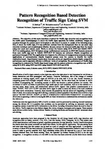
cross-validation set. Working with simulated data allowed us to generate enough validation data-points so that we can safely state that the best (with respect to generalization) network parameter values found are indeed optimal. The other advantage of the artificial databases is that we can experiment with different input domain dimensionalities, the number of output classes and the amount of inter-class overlap. Specifically, as it will become apparent from the experimental results, the optimum epsilon value is dependent on the amount of inter-class overlap that is present in the data. A. Artificial Databases In this paper we kept the dimensionality of the input patterns fixed, and equal to 2, and we experimented with the number of output classes (2, 4, or 6) and the amount of overlap amongst data belonging to different classes (overlap values of 5%, 15%, 30% and 40% were used). The artificial databases consist of Gaussianly distributed data. Input patterns were drawn from either 2 or 4 or 6 classes. Qualitatively the overlap can be classified as low (5%), medium (15%) or high (30% or 40%). The amount of overlap of the simulated data was defined to be the error rate of the optimum Bayes classifier designed as pertinent to the data. For instance, if the Bayes classifier for a simulated data set exhibited a misclassification rate of x%, then the amount of overlap corresponding to this data-set was defined to be x%. For each one of the above 12 sets of artificial data (3 different number of classes × 4 different degrees of class overlap) we generated a training set, a validation set and a test set of 500, 5,000 and 5,000 data-points respectively. In Fig. 1 we show a scatter plot of the training data used for a 2, 4 and 6 class problem with 5% overlap.
Fig. 1. Scatterplots of data points for 2 class, 4 class and 6 class problems with 5% overlap.
B. Observations The major observations from our experiments are identified and elaborated below. Higher overlap data domains are well suited for the semisupervised learning approach. The validity of the above statement can be gathered from the plots in Fig. 2, where the x-coordinate represents the PCC XV (percent correct classification on the cross-validation set) value, while the ycoordinate represents the corresponding PCC Train (percent
Fig. 2. The plots represent the Percentage of Correct Classification on the Cross-validation set (PCC XV) versus the Percentage of Correct Classification over the training set (PCC Train). The best PCC XV values occur at PCC Train values that are less than 100%. This effect is amplified when the data overlap in data increases. Generalization performance is enhanced when there is some residual training error present after training is completed.
and RCE networks (again, they are omitted due to lack of space). Epsilon vs PCC Test performance for EAM for 4 class data of varying overlaps
95
90 PCC Test - Percentage correct classification on test set
correct classification on the training set) value. It is worth noting from these figures that, as the amount of overlap amongst the data increases, the best PCC XV values occurs at values of PCC Train that are further away from the 100% training performance that completely supervised networks (such as EAM) enforce. This is a manifestation of the overtraining issue associated with neural networks that has been often been reported in the literature. As we see from Fig. 2 the issue of over-training and its detrimental effects gradually becomes more pronounced as the amount of overlap in a problem increases. In other words, training the network to perfection affects the generalization performance of the network more severely for higher overlap values than for lower overlap values. It is worth mentioning that although the results in Fig. 2 correspond to EAM, similar type of results and associated conclusions correspond to FAM and RCE networks (they are omitted due to lack of space).
05% overlap
85
80 15% overlap
75
70
65 25% overlap
60 30% overlap
55
50
The “best epsilon value” migrates from lower to higher values for increasing data overlap. In Fig. 3 we depict the PCC Test and the PCC XV for epsilon values ranging from 0 to 1 with step 0.1. Note that a value of ε equal to 0 represents EAM. As it can be seen from the figure the best ε value for the low overlap case (overlap of 5%) is equal to 0.1, while the best ε value for the high overlap case (overlap of 40%) is equal to 0.8. This result is intuitively pleasing. For low overlap data overlapping data are scarcely witnessed. As a result, there is a lesser need for categories to expand and allow high errors in the training, in an effort to avoid overtraining. On the other hand high overlap data cause overtraining. By incorporating higher ε values when data overlap is high, categories are allowed to expand in a way that patterns of the erroneous label are incorporated within them, thus sidestepping the over-training issue. Hence, by avoiding over-training, higher generalization performances are observed for higher ε values when the data overlap is high. Once more, although the figures depict the results pertaining to EAM networks, similar types of results are valid for FAM
40% overlap
45
0
0.1
0.2
0.3
0.4
0.5
0.6
0.7
0.8
0.9
1
Epsilon
Fig. 3. Percentage of Correct Classification on Test set (PCC Test) versus epsilon for ssEAM. As the data overlap increases, the best epsilon value migrates towards 1, indicating the need for less supervision.
Better compression rates are achieved at higher epsilon values. This is an obvious result because higher ε values allow more error during training with the direct effect of creating fewer categories. In Fig. 4 we depict the number of categories created by ssEAM for different ε values and for the 2 class 40% overlap dataset. What is worth mentioning regarding this figure is that the ε value that achieves the highest generalization performance on the test set does not necessarily create a network with the highest number of categories. On the contrary, the number of categories created at the value of ε that maximizes generalization is relatively small, at times amongst the smallest number observed for all ε values.
Categories created and PCC vs Epsilon
PCC Test vs Epsilon for FAM and EAM 74
54 247
ssEAM ssFAM
result on 4 class 25% overlap data
53 72
52 185
Percentage Correct Classification
best classification 165
51
good compression 142
PCC Test
50 Actual number of categories created by EAM
49
86 48 64 47
68
66
64
35 26
46
45
70
optimum epsilon
8
26
PCC Test Categories
62
6
60
0
0.1
0.2
0.3
0.4
0.5
0.6
0.7
0.8
0.9
1
Epsilon
0
0.1
0.2
0.3
0.4
0.5 Epsilon
0.6
0.7
0.8
0.9
1
Fig. 4. Categories created and Percentage Correct Classification over Testing set (PCC Test) against epsilon. Note the drastic fall in the number of categories created from 247 by EAM to 35 by the best ssEAM. The epsilon parameter ushers not only better classification but also good compression.
Fig. 6. Percentage Correct Classification on Test set (PCC Test) of ssEAM and ssFAM against epsilon. An optimum epsilon value for one type of network is generally a good epsilon value for another type of network too.
Performance gains are universal. In the previous plots we have depicted the performance of the best possible network for each specific ε (the one achieving the highest generalization performance on the validation set with respect to the remaining network parameters; e.g., ρ, a, µ and order of training pattern presentation for EAM). Fig. 5 depicts the generalization performance of the best network, and the average performance of all the networks that we have experimented with. What is worth mentioning from this figure is that the peak average performance of all the networks coincides with the performance of the best network at the optimal ε value.
Furthermore, beyond this optimum ε value we notice that the average generalization performance of all the networks exhibits a monotonically decreasing behavior with increasing ε values.
PCC Test and Average PCC XV vs Epsilon for ssFAM on a 4 class 15% overlap dataset
90
The optimal epsilon value for one network is a good epsilon value for the other networks too. For illustration purposes please refer to Fig. 6, where the performance results of all ssFAM and ssEAM with a 4-class problem and 25% overlap is depicted. This result is an additional testament to the goodness of the best ε value for a particular data set. Hence, the best ε value obtained for a particular data set can be considered more or less independent of the semisupervised classifier that is employed for classification purposes.
80
Percentage correct classification
70
60
50
40 Best PCC Test for each epsilon value
30
Average PCC XV (average over 20,000 experiments) for each epsilon
20
10
0
0
0.1
0.2
0.3
0.4
0.5 Epsilon
0.6
0.7
0.8
0.9
1
Fig. 5. PCC Test of best ssEAM network and average PCC XV versus epsilon. The peaks coincide, assuring that the gains witnessed are universal and not limited to the best network alone.
Optimizing with respect to epsilon makes good sense. If we compare the performance of semi-supervised networks with fully supervised networks across all the experiments that we have performed we observe the following: the generalization performance of the best semi-supervised network outperformed the generalization performance of the best fully supervised network by 0.14% in the worst case and by 11.06% in the best case with an average of around 6.5% performance enhancement. Furthermore, the ratio of utilized categories achieved by the best semi-supervised networks compared to the best fully supervised network was around 10. Similar types of qualitative results were observed, when the best ssFAM was compared to the best FAM and the best ssRCE was compared with the best RCE.
TABLE 1: BEST EAM, ssEAM, FAM AND ssFAM FOR ALL DATASETS IN TERMS OF PCC TEST Best Best ssEAM Best Best ssFAM Overlap EAM @optimum epsilon FAM @optimum epsilon 2 class 5%
89.3
15%
76.1
25%
63.2
30%
62.1
40%
54.2
95.22 @ 0.4 * 85.24 @ 0.7 * 75.36 @ 0.6 70.46 @ 0.4 60.5 @ 0.8 *
89.9 74.9 63 61.7 53.3
95.1 @ 0.1 * 85.02 @ 0.2 * 75.18 @ 0.4 70.28 @ 0.6 * 60.22 @ 0.7
4 class 5%
91.3
15%
75.8
25%
60.8
30%
58.6
40%
47.3
91.8 @ 0.1 81.5 @ 0.4 70.24 @ 0.5 67.2 @ 0.6 58.32 @ 0.8
92.3 75.5 62 57.6 48.6
94.14 @ 0.1 84.74 @ 0.2 72.06 @ 0.5 63.52 @ 0.5 55.64 @ 0.7
6 class 5%
88.4
15%
78.1
25%
61.5
30%
56.7
40%
46.2
89.07 @ 0.1 78.24 @ 0.2 66.07 @ 0.3 62.69 @ 0.5 49.96 @ 0.7 *
85.6 69.3 58.4 58.2 42.2
86.91 @ 0.1 74.34 @ 0.2 61.99 @ 0.6 60.05 @ 0.2 52.68 @ 0.3
* - Indicates presence of more than one optimum value of epsilon.
Finally, in Table I we list for every pattern recognition task we considered in our experiments the test performance of the best EAM, ssEAM, FAM and ssFAM classifier. As it can be witnessed, semi-supervised classifiers outperform their fully supervised counterparts in all experiments. The difference in test performance is especially pronounced, when the degree of class overlap is higher than low (5%).
IV. CONCLUSIONS In this paper we have presented the concept of semisupervised learning (SSL) as it is applied to exemplar-based classifiers (EBC). SSL refers to the semi-supervised construction of clusters during the training phase of these classifiers. We have demonstrated the merits of SSL by conducting a series of experiments using artificially generated data sets and implementing SSL-variants of Ellipsoid ARTMAP, Fuzzy ARTMAP and the planar Restricted Coulomb Energy classifier. Apart from lending the capability of coping with inconsistent training patterns and non-stationary pattern recognition problems, EBCs that follow the SSL paradigm exhibit improved generalization performance, while employing only a small number of exemplars, when compared to their fully supervised versions. REFERENCES [1]
S. Grossberg, “Adaptive pattern recognition and universal encoding II: feedback, expectation, olfaction, and illusions,” Biological Cybernetics, vol. 23, pp. 187-202, 1976. [2] V.N. Vapnik, The Nature of Statistical Learning Theory, Springer Verlag, New York, NY, 1995. [3] V.N. Vapnik, Statistical Learning Theory, John Wiley & Sons, New York, NY, 1998. [4] G.C. Anagnostopoulos, M. Georgiopoulos, S.J. Verzi, and G.L. Heileman, “Reducing generalization error and category proliferation in Ellipsoid ARTMAP via tunable misclassification error tolerance: Boosted Ellipsoid ARTMAP,” Proceedings of the IEEE-INNS-ENNS International Joint Conference on Neural Networks (IJCNN ’02), vol. 3, pp 2650-2655, Honolulu, Hawaii, July 2002. [5] G.C. Anagnostopoulos and M. Georgiopoulos, “Ellipsoid ART and ARTMAP for incremental unsupervised and supervised learning,” Proceedings of the IEEE-INNS-ENNS International Joint Conference on Neural Networks (IJCNN ’01), vol. 2, pp. 1221-1226, Washington, Washington D.C., July 2001. [6] G.C. Anagnostopoulos, “Novel approaches in Adaptive Resonance Theory for machine learning,” Doctoral Dissertation, University of Central Florida, Orlando, Florida, 2001. [7] S.J. Verzi, G.L. Heileman, M. Georgiopoulos and M. J. Healy, “Rademacher penalization applied to Fuzzy ARTMAP and Boosted ARTMAP,” Proceedings of the IEEE-INNS-ENNS International Joint Conference on Neural Networks (IJCNN ’01), vol. 2, pp. 1191-1196, Washington, Washington D.C., July 2001. [8] G.A. Carpenter, S. Grossberg, N. Markuzon, J.H. Reynolds and D.B. Rosen, “Fuzzy ARTMAP: A neural network architecture for incremental supervised learning of analog multidimensional maps,” IEEE Transaction on Neural Networks, vol. 3:5, pp. 698-713, 1992. [9] M.H. Hassoun, Fundamentals of Artificial Neural Networks, MIT Press, Cambridge, Massachusetts, 1995. [10] M. Stone, “Cross-validatory choice and assessment of statistical predictions,” Journal of the Royal Statistical Society, vol. B36, pp. 111133, 1974.