Wavelet Algorithms for High-Resolution Image Reconstruction

Wavelet Algorithms for High-Resolution Image Reconstruction Raymond H. Chan, Tony F. Chany, Lixin Shenz, Zuowei Shenz April 29, 2002

Abstract

High-resolution image reconstruction refers to reconstructing high-resolution images from multiple low-resolution, shifted, degraded samples of a true image. In this paper, we analyze this problem from the wavelet point of view. By expressing the true image as a function in L2(R2 ), we derive iterative algorithms which recover the function completely in the L2 sense from the given low-resolution functions. These algorithms decompose the function obtained from the previous iteration into dierent frequency components in the wavelet transform domain and add them into the new iterate to improve the approximation. We apply wavelet (packet) thresholding methods to denoise the function obtained in the previous step before adding it into the new iterate. Our numerical results show that the reconstructed images from our wavelet algorithms are better than that from the Tikhonov least squares approach. Extension to super-resolution image reconstruction, where some of the low-resolution images are missing, is also considered.

1 Introduction Many applications in image processing require deconvolving noisy data, for example the deblurring of astronomical images [11]. The main objective in this paper is to develop algorithms for these applications using wavelet approach. We will concentrate on one such application, namely, the high-resolution image reconstruction problem. High-resolution images are often desired in many situations, but made impossible because of hardware limitations. Increasing the resolution by image processing techniques [1, 3, 9, 14, 15, 22, 23, 24] is of great importance. Here we consider creating high-resolution images of a scene from the low-resolution images of the same scene. When we have a full set of low-resolution images, the problem is referred to as high-resolution image reconstruction; and when only some of the low-resolution images are available, the problem is called super-resolution image reconstruction. In both cases, the low-resolution images are obtained from sensor arrays which are shifted from each others with subpixel displacements. The reconstruction of the high-resolution image can be modeled as solving a linear system Lf = g, where L is the convolution operator, g is a vector formed from the low-resolution images, and f is the desired high-resolution image, see [1]. In this paper, we look at this problem from the wavelet point of view and analyze the process through multiresolution analysis. The true image can be considered as a function f in L2 (R2 ) and Department of Mathematics, the Chinese University of Hong Kong, Shatin, NT, P. R. China. Research supported in part by HKRGC Grant CUHK4212/99P and CUHK Grant DAG 2060183. y Department of Mathematics, University of California, Los Angeles, Los Angeles, CA 90024-1555, USA. Research supported in part by the ONR under contract N00014-96-1-0277 and by the NSF under grant DMS-9973341 z Department of Mathematics, National University of Singapore, 2 Science Drive 2, Singapore 117543. Research supported in part by the Centre of Wavelets, Approximation and Information Processing (CWAIP) funded by the National Science and Technology Board, the Ministry of Education under Grant RP960 601/A. 

1

the low-resolution images can be thought of as the low-frequency samples of f obtained by passing f through some lowpass lters. Thus the problem can be posed as reconstructing a function from the given multiple low-frequency samples of f . To recover f , we deconvolve iteratively the high-frequency components of f which are hidden in the low-frequency samples. Our iterative process decomposes the function obtained in the previous iteration into dierent frequency components in the wavelet transform domain and then adds them to the new iterate to improve the approximation. In this setting, it is easy to apply wavelet methods to denoise the function obtained in the previous step before adding it into the new iterate. The high-resolution image reconstruction problem is closely related to the deconvolution problem. In the recent works of [12] and [13], an analysis of minimizing the maximum risk over all the signals in a set of signals is given. Then, it was applied to estimate the risk of the wavelet thresholding method used on the deconvoluted signals. Their wavelet thresholding algorithm is proven to be close to the optimal risk bound when a mirror wavelet basis is used. The main diculty in denoising deconvoluted signals is that when the convolution lowpass lter has zeros at high frequency, the noise variance in the solution has a hyperbolic growth [12]. To overcome this diculty, a mirror wavelet basis is constructed to de ne a sparse representation of all the signals in the set of given signals and to nearly diagonalize the covariance operator of the noise in the deconvoluted solution in order to reach the optimal risk bound. The approach here is dierent. The highpass lters are added to perturb the zeros of the convolution kernel to prevent the noise variance from blowing up. Our wavelet (packet) thresholding method, which is a wavelet denoising method, is built into each iterative step so as to remove the noise from the original data. It also keeps the features of the original signal while denoising. In this sense, our method is more related to the Tikhonov least squares method where a regularization operator is used to perturb the zeros of the convolution kernel and a penalty parameter is used to damp the high-frequency components for denoising. Since the least squares method penalizes the high-frequency components of the original signal at the same rate as that of the noise, it smoothens the original signal. In contrast, our thresholding method penalizes the high-frequency components of the signal in a rate signi cantly lower than that of the noise, and hence it will not smoothen the original signal in general. Moreover, there is no need to estimate the regularization parameter in our method. Our numerical tests show that the reconstructed images are of better quality. Also our algorithms can easily be extended to the super-resolution case. The outline of the paper is as follows. In x2, we give a mathematical model of the high-resolution image reconstruction problem. In x3, we derive our algorithms. Extensions to the super-resolution case are also discussed there. Numerical examples are given in x4 to illustrate the eectiveness of the algorithms. After the concluding remarks, we provide in the Appendix an analysis of our algorithms via the multiresolution analysis.

2 The Mathematical Model Here we give a brief introduction to the mathematical model of the high-resolution image reconstruction problem. Details can be found in [1]. Suppose the image of a given scene can be obtained from sensors with N1  N2 pixels. Let the actual length and width of each pixel be T1 and T2 respectively. We will call these sensors low-resolution sensors. The scene we are interested in, i.e. the region of interest, can be described as:  S = (x1 ; x2 ) 2 R2 j 0  x1  T1 N1; 0  x2  T2 N2 : Our aim is to construct a higher resolution image of the same scene by using an array of K1  K2 low-resolution sensors. More precisely, we want to create an image of S with M1  M2 pixels, where 2

M1 = K1 N1 and M2 = K2 N2 . Thus the length and width of each of these high-resolution pixels will be T1 =K1 and T2 =K2 respectively. To maintain the aspect ratio of the reconstructed image, we consider only K1 = K2 = K . Let f (x1 ; x2 ) be the intensity of the scene at any point (x1 ; x2 ) in S. By reconstructing the high-resolution image, we mean to nd or approximate the values

K 2 Z (i+1)T1 =K Z (j+1)T2 =K f (x ; x )dx dx ; 0  i < M ; 0  j < M ; 1 2 1 2 1 2 T1 T2 iT1 =K jT2 =K

which is the average intensity of all the points inside the (i; j )th high-resolution pixel:

T

 T  T T 1 2 2 i K ; (i + 1) K  j K ; (j + 1) K ; 0  i < M1 ; 0  j < M2 : 1

(1)

In order to have enough information to resolve the high-resolution image, there are subpixel displacements between the sensors in the sensor arrays. Ideally, the sensors should be shifted from each other by a value proportional to the length and the width of the high-resolution pixels. More precisely, for sensor (k1 ; k2 ), 0  k1 ; k2 < K , its horizontal and vertical displacements dxk1 k2 and dyk1 k2 with respect to the point (0; 0) are given by

dxk1 k2









= k1 + 1 ?2 K TK1 and dyk1 k2 = k2 + 1 ?2 K TK2 :

For this low-resolution sensor, the average intensity registered at its (n1 ; n2 )th pixel is modeled by:

gk1 k2 [n1 ; n2 ] = T 1T 1

2

ZT

x 1 (n1 +1)+dk1 k2

T1 n1 +dxk1 k2

ZT

y 2 (n2 +1)+dk1 k2

T2 n2 +dyk1 k2

f (x1 ; x2 )dx1 dx2 + k1 k2 [n1 ; n2 ]:

(2)

Here 0  n1 < N1 and 0  n2 < N2 and k1 k2 [n1 ; n2 ] is the noise, see [1]. We remark that the integration is over an area the same size of a low-resolution pixel. Notice that using the mid-point quadrature rule and neglecting the noise k1 k2 [n1 ; n2 ] for the moment,   1 1 y x gk1 k2 [n1 ; n2 ]  f T1 (n1 + 2 ) + dk1 k2 ; T2 (n2 + 2 ) + dk1 k2  T 1 T 1 2 1 = f K (Kn1 + k1 + 2 ); K (Kn2 + k2 + 2 ) : Thus if we intersperse all the low-resolution images gk1 k2 to form an M1  M2 image g by assigning

g[Kn1 + k1 ; Kn2 + k2 ] = gk1 k2 [n1 ; n2 ]; then

T



(3)

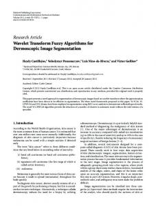
g[i; j ]  f K (i + 12 ); TK2 (j + 12 ) ; 0  i < M1 ; 0  j < M2 which is the value of f at the mid-point of the (i; j )th high-resolution pixel in (1). Thus g is an approximation of f . Figure 1 shows how to form a 4  4 image g from four 2  2 sensor arrays fgk1 k2 g1k1 ;k2=0 where all gk1 k2 have 2  2 pixels. The image g, called the observed high-resolution image, is already a better image (i.e. better approximation to f ) than any one of the low-resolution samples gk1 ;k2 themselves, see Figures 4 (a){(c) in x4. 1

3

a1

a2

b1

b2

a3

a4

b3

b4

g00

g01

............. ..........

c1

c2

d1

d2

c3

c4

d3

d4

a1

b1

a2

b2

c1

d1

c2

d2

a3

b3

a4

b4

c3

d3

c4

d4

g

g10

g11 .

Figure 1: Construction of the observed high-resolution image. To obtain an even better image than the observed high-resolution image g, one will have to solve (2) for f . According to [1], we solve it by rst discretizing it using the rectangular quadrature rule. Or equivalently, we assume that for each (i; j )th high-resolution pixel given in (1), the intensity f is constant and is equal to f [i; j ] for every point in that pixel. Then carrying out the integration in (2), and using the re-ordering (3), we obtain a system of linear equations relating the unknown values f [i; j ] to the given low-resolution pixel values g[i; j ]. This linear system, however, is not square. This is because the evaluation of gk1 k2 [n1 ; n2 ] in (2) involves points outside the region of interest S. For example, g0;0 [0; 0] requires the values f (x1 ; x2 ) where x1 < 0 and x2 < 0, i.e. it involves f [?1; ?1]. Thus we have more unknowns than given values, and the system is underdetermined. To compensate for this, one imposes boundary conditions on f for xi outside the domain. A standard way is to assume that f is periodic outside:

f (x + iT1 N1 ; y + jT2 N2 ) = f (x; y);

i; j 2 Z;

see for instance [8, x5.1.3]. Other boundary conditions, such as the symmetric (also called Neumann or re ective) boundary condition and the zero boundary condition, can also be imposed, see [1, 18]. We emphasize that these boundary conditions will introduce boundary artifacts in the recovered images, see for examples Figures 4 (d){(f) in x4. For simplicity, we will only develop our algorithms for periodic boundary conditions here. For other boundary conditions, similar algorithms can be derived straightforwardly. Using the periodic boundary condition and ordering the discretized values of f and g in a rowby-row fashion, we obtain an M1 M2  M1 M2 linear system of the form:

Lf = g:

(4)

L = L x Ly

(5)

The blurring matrix L can be written as

4

where is the Kronecker tensor product and Lx is the M1  M1 circulant matrix with the rst row given by   1 1; : : : ; 1; 1 ; 0; : : : ; 0; 1 ; 1; : : : ; 1 : K 2 2 Here the rst K=2 entries are equal to 1. We note that the last K=2 nonzero entries are there because of our periodic assumption on f . The M2  M2 blurring matrix Ly is de ned similarly. We note that the matrix L is a block-circulant-circulant-block (BCCB) matrix. Thus (4) can be solved by using three 2-dimensional Fast Fourier Transforms (FFTs) in O(M1 M2 log(M1 M2 )) operations, see for instance [8, x5.2.2]. As examples, the matrices Lx for the cases of 2  2 and 4  4 sensor arrays are given respectively by: 3 22 2 1 1 2 3 22 1 66 2 2 2 1 1 77 1 77 77 66 1 2 2 2 1 66 1 2 1 1 1 7 6 6 L2  4 66 . . . . . . . . . 77 and L4  8 66 . . . . . . . . . . . . . . . 777 : (6) 7 6 5 4 1 2 2 2 17 1 2 1 64 1 1 2 2 25 1 1 2 2 1 1 2 2 Because (2) is an averaging process, the system in (4) is ill-conditioned and susceptible to noise. To remedy this, one can use the Tikhonov regularization which solves the system (L L + R)f = L g:

(7)

Here R is a regularization operator (usually chosen to be the identity operator or some dierential operators) and > 0 is the regularization parameter, see [8, x5.3]. If the boundary condition of R is chosen to be periodic, then (7) is still a BCCB system and hence can be solved by 3 FFTs in O(M1 M2 log(M1 M2 )) operations. If the symmetric boundary condition is used, then (7) is a block Toeplitz-plus-Hankel system with Toeplitz-plus-Hankel blocks. It can be solved by using three 2-dimensional fast cosine transforms (FCTs) in O(M1 M2 log(M1 M2 )) operations, see [18]. We note that (7) is derived from the least squares approach of solving (4). In the next section, we will derive algorithms for nding f by using the wavelet approach. They will improve the quality of the images when compared with (7).

3 Reconstruction In this section, we analyze the model given in x2 using the wavelet approach. Since (2) is an averaging process, the matrices in (6) can be considered as a lowpass ltering acting on the image f with a tensor product re nement mask, say a. Let  be the tensor product bivariate re nable function with such a re nement mask. Here, we recall that a function  in L2 (R2 ) is re nable if it satis es

=4

X

2Z2

a()(2
?):

The sequence a is called a re nement mask, or lowpass lter. The symbol of the sequence a is de ned as X ba(!) := a()e?i! : 2Z2

5

The function  is stable if its shifts (integer translates) form a Riesz system, i.e. there exist constants 0 < c  C < 1, such that for any sequence q 2 `2 (Z2),

X ckqk  q()(
? )  C kqk : 2

Stable functions  and

d

2

2Z

2

(8)

2

are called a dual pair when they satisfy  h; d (
? )i = 01;;  2= Z0;2 n f(0; 0)g:

We will denote the re nement mask of d by ad . For a given compactly supported re nable stable function  2 L2 (R2 ), de ne S ()  L2 (R2 ) to be the smallest closed shift invariant subspace generated by  and de ne S k () := fu(2k
) : u 2 S ()g; k 2 Z: Then the sequence S k (), k 2 Z, forms a multiresolution of L2 (R2 ). Here we recall that a sequence S k () forms a multiresolution when the following conditions are satis ed: (i) S k ()  S k+1 (); (ii) [k2ZS k () = L2(R2 ) and \k2ZS k () = f0g; (iii)  and its shifts form a Riesz basis of S (), see [5]. The sequence S k (d ), k 2 Z, also forms a multiresolution of L2 (R2 ). The tensor product of univariate re nable functions and wavelets used in this paper will be derived from the following examples. Example 1 ([5, p.277]). For 2  2 sensor arrays, using the rectangular rule for (2), we get L2 in (6). Correspondingly, the re nement mask m is the piecewise linear spline, i.e. m(?1) = 41 ; m(0) = 12 ; m(1) = 14 ; and m() = 0 for all other . The nonzero terms of the dual mask of m used in this paper are: md (?2) = ? 18 ; md (?2) = 14 ; md (0) = 34 ; md (1) = 14 ; md (2) = ? 81 : In general, the tensor product bivariate lters for the dilation 2I , where I is the identity matrix, are generated as follows. Let  and d be a dual pair of the univariate re nable functions with re nement masks m and md respectively. Then, the biorthonormal wavelets and d are de ned by X X := 2 r()(2
?); and d := 2 rd ()d (2
?); where

2Z

2Z

r() := (?1) md (1 ? ); and rd () := (?1) m(1 ? )

are the wavelet masks, see for example [5] for details. The tensor product dual pair of the re nement symbols are given by ba(!) = m b (!1 )mb (!2), bad (!) = mb d(!1 )mb d(!2 ), and the corresponding wavelet symbols are bb(0;1) (!) = m b (!1)rb(!2 ), bbd(0;1) (!) = mb d(!1 )rbd(!2), bb(1;0) (!) = rb(!1 )mb (!2), bbd(1;0) (!) = rbd(!1 )mb d (!2 ), bb(1;1) (!) = rb(!1 )rb(!2 ), bbd(1;1) (!) = rbd (!1 )rbd(!2 ), where ! = (!1 ; !2 ). Although we only give here the details of re nable functions and their corresponding wavelets with dilation 2I , the whole theory can be carried over to the general isotropic integer dilation matrices. The details can be found in [10] and the references therein. In the next example, we give the re nable and wavelet masks with dilation 4I that are used to generate the matrices for 4  4 sensor arrays. 6

Example 2. For 4  4 sensor arrays, using the rectangular rule for (2), we get L in (6). The 4

corresponding mask is

m() = 18 ; 14 ; 14 ; 14 ; 18 ;  = ?2; : : : ; 2;

with m() = 0 for all other . It is the mask of a stable re nable function  with dilation 4 (see e.g. [16] for a proof). The nonzero terms of a dual mask of m is 1 ; 1 ; 5 ; 1 ; 5 ; 1 ; ? 1 ;  = ?3; : : : ; 3: md() = ? 16 8 16 4 16 8 16 The nonzero terms of the corresponding wavelet masks (see [20]) are r1 () = ? 18 ; ? 14 ; 0; 14 ; 81 ;  = ?2; : : : ; 2; 1 ; ? 1 ; 5 ; ? 1 ; 5 ; ? 1 ; ? 1 ;  = ?2; : : : ; 4; r2 () = ? 16 8 16 4 16 8 16 1 ; 1 ; ? 7 ; 0; 7 ; ? 1 ; ? 1  = ?2; : : : ; 4: r3 () = 16 8 16 16 8 16 The dual wavelet masks are

r1d () = (?1)1? r3 (1 ? ); r2d () = (?1)1? m(1 ? ); r3d () = (?1)1? r1 (1 ? ); for appropriate . In the next two subsections, we will use the wavelet approach to design algorithms for recovering the high-resolution image from the low-resolution images of a true image. In x3.1, we rst consider the true image as a representation of a function in certain subspace of L2 (R2 ) and using wavelet means we recover this function from the given set of low-resolution images. In x3.2, we translate the wavelet algorithms into matrix terminologies.

3.1 Function Reconstruction

Since S k (d ), k 2 Z, forms a multiresolution of L2 (R2 ), we can assume without loss of generality that the pixel values of the original image are the coecients of a function f in S k (d ) for some k. The pixel values of the low-resolution images can be considered as the coecients of a function g in S k?1 (d ) and its 1=2k translates, i.e. g is represented by d (2k?1 (
? =2k )) with  2 Z2. The lowresolution images keep most of the low-frequency information of f and the high-frequency information in f is folded by the lowpass lter a. Hence, to recover f , the high-frequency information of f hidden in the low-resolution images will be unfolded and combined with the low-frequency information to restore f . We will unfold the high-frequency content iteratively using the wavelet decomposition and reconstruction algorithms. For 2  2 sensor arrays, the multiresolution analysis S k (d ) used is from a re nable function with dilation matrix 2I . In general, K  K sensor arrays can be analyzed by the multiresolution analysis generated by a re nable function with dilation matrix K
I . For simplicity, we give the analysis for the case that the dilation matrix is 2I and k = 1. A similar analysis can be carried out for more general cases. Let f 2 S 1 (d ). Then,

f=

X

hf; 2(2
?)i2d (2
?) := 2

2Z2

7

X

2Z2

v()d (2
?):

(9)

The numbers v(),  2 Z2, are the pixel values of the high-resolution image we are seeking, and they form the discrete representation of f under the basis 2d (2
?),  2 Z2. The given data set a  v() is the observed high-resolution image. By using the re nability of d , one nds that a  v is the coecient sequence of the function g represented by d (
? =2),  2 Z2, in S 1 (d ). We call this g the observed function and it is given by X (10) g := (a  v)()d (
? =2): 2Z2

The observed function can be obtained precisely once a  v is given. When only a  v is given, to recover f , one rst nds v from a  v; then, derives f using the basis 2d (2
?),  2 Z2, as in (9). Here we provide an iterative algorithm to recover v. At step (n + 1) of the algorithm, it improves the high-frequency components of f by updating the highfrequency components of the previous step. The algorithm is presented in the Fourier domain where the problem becomes: for a given ad  v = bavb, one needs to nd vb in order to restore f . Our algorithm will make use of the following fact from the biorthogonal wavelet theory: for a given tensor product bivariate re nement mask a corresponding to a stable re nable function , one can nd a tensor product dual mask ad and the corresponding wavelet masks b and bd ,  2 Z22, such that the symbols of the re nement masks and wavelet masks satisfy the following equation:

badba +

X bdb b b = 1:

 2Z nf(0;0)g 2 2

(11)

We note that when the re nable function  (of the convolution kernel a) and its shifts form an orthonormal system (e.g. in the Haar case), then (11) holds if we choose bad = ba and bbd = bb . This leads to orthonormal wavelets. When  and its shifts form only a Riesz system, one has to use biorthogonal wavelets.  v + (P bbdbb )vb. Hence we have the following algorithm. By (11), we have bv = bad ad

Algorithm 1.

(i) Choose vb0 2 L2 [?; ]2 ;

(ii) Iterate until convergence:

0 1 X bbdbb A vbn: vbn = bad ad v+@ +1

 2Z nf(0;0)g 2 2

(12)

 v = badbavb in the right hand side of (12) represents the approxiWe remark that the rst term bad ad mation of the low-frequency components of f whereas the second term improves the high frequency approximation. Given bvn , fn is de ned via its Fourier transform as: fbn(
) := vbn (
=2)bd (
=2) 2 S 1 (d ): (13) We now show that the functions fn converge to the function f in (9). Proposition 1. Let  and d be a pair of dual re nable functions with re nement masks a and ad and let b and bd ,  2 Z22 n f(0; 0)g, be the wavelet masks of the corresponding biorthogonal wavelets. Suppose that 0  badba  1 and its zero set has measure zero. Then, the sequence vbn de ned in (12) converges to vb in the L2 -norm for any arbitrary vb0 2 L2 [?; ]2 . In particular, fn in (13) converges to f in (9) in the L2 -norm. 8

Proof. For an arbitrary vb0 2 L2 [?; ]2 , applying (12), we have

1n 0 X bbdbb A (vb ? vb ): bv ? vbn = @ 0

 2Z22nf(0;0)g

It follows from 0  badba  1 and (11) that

X bbdbb  1:    2Z nf ; g 2 2

(0 0)

Since badba  0 and its zero set has measure zero, the inequality

X bbdbb < 1    2Z nf ; g 2 2

(0 0)

holds almost everywhere. Hence,

0 1n X bbdbb A (vb ? vb ) ! 0; @ 0

 2Z nf(0;0)g 2 2

as n ! 1 a.e.:

By the Dominated Convergence Theorem (see e.g. [19]), vbn converges to vb in the L2 -norm. Since d (
? ) is a Riesz basis of S 0 (d ), from (8), 2d (2
?) is a Riesz basis of S 1 (d ). Hence by (8) again,

kfn ? f k = k 2

X

2Z

 Ck

(vn () ? v())2(2
?)k2

2

X

(vn () ? v())k2 = 2C kvbn ? vbk2 ?! 0:

2Z2

Remark 1. The symbols of the re nement masks and the corresponding dual masks used in this paper are tensor products of univariate ones that satisfy the assumptions of this proposition. Remark 2. The above convergence result is also applicable to the super-resolution case. Assume for simplicity that a  v is downsampled to four sub-samples a  v( ? 2),  2 Z . For the super-resolution case, one only has some of the sub-samples, a  v( ? 2),  2 A  Z . In this case, one rst applies 2 2

2 2

an interpolatory scheme (e.g. [10]) to obtain the full set of the sample w approximately. Let the `2 solution of the equation a  z = w be u. Then, a  u( ? 2) = a  v( ? 2) for  2 A. Applying Algorithm 1 to a  u, the above proposition asserts that it converges to u.

When there are noise in the given data a  v, one may subtract some high-frequency components from vbn at each iteration to reduce the noise, since noise is in the high-frequency components. Then we get the following modi ed algorithm: 9

Algorithm 2.

(i) Choose vb0 2 L2 [?; ]2 ;

(ii) Iterate until convergence:

1 0 X bbdbb A vbn; vbn = bad ad  v + (1 ? ) @ +1

 2Z nf(0;0)g 2 2

0 < < 1:

(14)

In this denoising procedure, the high-frequency components are penalized uniformly by the factor (1 ? ). This smoothens the original signals while denoising. To remedy this, we now introduce a wavelet thresholding denoising method. It is based on the 2 observation that bb c vn = b\   vn ,  2 Z2 n f(0; 0)g, is the exact wavelet coecients of the wavelet decomposition (without downsampling) of the function fn , the nth approximation of f . A further decomposition of b  vn , by using the lowpass lter a and the highpass lters b several times, will give the wavelet coecients of the decomposition of fn by the translation invariant wavelet packets de ned by the biorthogonal lters a, ad and b and bd (see e.g. [17] and [25]). More precisely, by using (11) we have

bb vbn = bad J (ba)J bb vbn + X badj J ?1 j =0

X bdb j b b b (ba) b vbn ;

2Z22nf(0;0)g

where J is the number of levels used to decompose bb vbn . For each j and 2 Z22 nf(0; 0)g, bb (ba)j bb vbn is the coecients of the wavelet packet (see e.g. [25]) down to the j th level. A wavelet thresholding denoising procedure is then applied to bb (ba)j bb vbn , the coecients of the wavelet packet decomposition of fn , before b  vn is reconstructed back by the dual masks. This denoises the function fn. Our method keeps the features of the original signal. Moreover, since we do not downsample (by a factor of 2) in the decomposition procedure, we are essentially using a translation invariant wavelet packet system [17], which is a highly redundant system. As was pointed out in [4] and [17], a redundant system is desirable in denoising, since it reduces the Gibbs oscillations. Another potential problem with Algorithm 2 is that at each iteration, vbn+1 inherits the noise from the observed data ad  v present in the rst term on the right hand side of (14). If the algorithm converges at the n0 -th step, then vbn0 still carries the noise from ad  v. One can eliminate part of these noise by passing the nal iterate vbn0 through the wavelet thresholding scheme we mentioned above (see Step (iii) below). We summarize our thresholding method in the following algorithm.

Algorithm 3.

(i) Choose vb0 2 L2 [?; ]2 ;

(ii) Iterate until convergence:

bvn

+1

where

v+ = bad ad

X bd b  b T b vbn ;

 2Z22nf(0;0)g

 J X  d j ba T (bb vbn) = bad (ba)J bb vbn + J ?1 j =0

X bd b j b  b D b (ba) b vbn ;

2Z22nf(0;0)g

and D is a thresholding operator (see for instant (19) below).

10

(iii) Let vbn0 be the nal iterate from Step (ii). The nal solution of our Algorithm is:

 J

vbc = bad (ba)J vbn0 +

X  d j ba

J ?1 j =0

X bd b j  b D b (ba) vbn ;

2Z22nf(0;0)g

0

where D is the same thresholding operator used in Step (ii).

In both the regularization method (Algorithm 2) and the thresholding method (Algorithm 3), the nth approximation fn is denoised before it is added to the iterate to improve the approximation. The major dierence between Algorithms 2 and 3 is that Step (ii) in Algorithm 2 is replaced by Step (ii) of Algorithm 3 where the thresholding denoising procedure is built in.

3.2 Image Reconstruction

Let us now translate the results above from wavelets notations into matrix terminologies. Denote by L, Ld , Hd and H the matrices generated by the symbols of the re nement and wavelet masks For the periodic boundary conditions, the matrix L is already given in ba, abd, bb and bbd respectively. (5) and the matrices Ld , Hd and H will be given in detail in x4. Using these matrices, (11) can be written as:

Ld L + Also (12) can be written as:

fn

+1

X

 2Z22nf(0;0)g

Hd H = I:

0 1 X Hd H A fn = Ld g + @  2Z22nf(0;0)g

(15)

(16)

where g ( a  v) is the observed high-resolution image given in (4) and fn are the approximations of f at the nth iteration. Rewriting (16) as 0 1

fn ? @ +1

X

 2Z22nf(0;0)g

Hd H A fn = Ld g;

one sees that it is a stationary iteration for solving the matrix equation

2 0 13 X 4I ? @ HdH A5 f = Ld g:  2Z22nf(0;0)g

Therefore by (15), we get the matrix form of Algorithm 1.

Algorithm 1 in Matrix Form: LdLf = Ld g: We note that there is no need to iterate on (16) to get f . 11

(17)

In a similar vein, one can show that Algorithm 2 is actually a stationary iteration for the matrix equation 0 1

@Ld L +

X

 2Z22nf(0;0)g

Hd H A f = Ld g:

By (15), this reduces to the following algorithm.

Algorithm 2 in Matrix Form:



Ld L +

I  f = 1 Ld g: 1? 1?

(18)

Again there is no need to iterate on (14) to get f . For periodic boundary conditions, both the matrices L and Ld in (18) are BCCB matrices of size M1 M2  M1 M2 and hence (18) can be solved eciently by using three 2-dimensional FFTs in O(M1 M2 log(M1 M2 )) operations, see [8, x5.2.2]. For symmetric boundary conditions, both matrices L and Ld are block Toeplitz-plus-Hankel matrices with Toeplitz-plus-Hankel blocks. Thus (18) can be solved by using three 2-dimensional FCTs in O(M1 M2 log(M1 M2 )) operations (see [18]). It is interesting to note that (18) is similar to the Tikhonov least squares method (7), except that instead of L , we use Ld . In (16), it is easy to further decompose H fn ,  2 Z22 n f(0; 0)g, by applying the matrices L and H , 2 Z22 n f(0; 0)g, to obtain the wavelet packet decomposition of fn. Then we can apply the threshold denoising method we have discussed in x3.1. To present the matrix form of Algorithm 3, we de ne Donoho's thresholding operator. For a given , let D((x1 ; : : : ; xl ; : : : )T ) = (t(x1 ); : : : ; t (xl ); : : : )T ; (19) where the thresholding function t is either (i) t (x) = xjxj>, referred to as the hard threshold, or (ii) t (x) = sgn(x) max(jxj ? ; 0), the soft threshold.

Algorithm 3 in Matrix Form:

(i) Choose an initial approximation f0 (e.g. f0 = Ld g);

(ii) Iterate until convergence:

fn = L d g + +1

Here

T (H fn

) = (Ld )J (L)J (H

f

 n) +

X  2Z22nf(0;0)g

X

J ?1 j =0

(Ld )j

p

HdT (H fn ) :

X

2Z22nf(0;0)g

?

H d Dn; H (L)j H fn




(20)

with Dn; given in (19) and n; = n; 2 log(M1 M2 ) where n; is the variance of H fn estimated numerically by the method provided in [7]. (iii) Let fn0 be the nal iterate from Step (ii). The nal solution of our Algorithm is

fc

= (Ld )J (L)J

fn0 +

X

J ?1 j =0

(Ld )j

X

2Z22nf(0;0)g

where Dn0 is the thresholding operator used in Step (ii).

12

?




H dDn0 H (L)j fn0 ;

According to [7], the choice of n; in Step (ii) is a good thresholding level for orthonormal wavelets as well as biorthonormal wavelets. The computational complexity of Algorithm 3 depends on the number of iterations required for convergence. In each iteration, we essentially go through a J -level wavelet decomposition and reconstruction procedure once, therefore it needs O(M1 M2 ) operations. As for the value of J , the larger it is, the ner the wavelet packet decomposition of fn will be before it is denoised. This leads to a better denoising scheme. However, a larger J will cost slightly more computational time. From our numerical tests, we nd that it is already good enough to choose J to be either 1 or 2. The variance n; is estimated by the method given in [7] which uses the median of the absolute value of the entries in the vector H fn . Hence the cost of computing n; is O(M1 M2 log(M1 M2 )), see for instance [21]. Finally, the cost of Step (iii) is less than one additional iteration of Step (ii). One nice feature of Algorithm 3 is that it is parameter-free | we do not have to choose the regularization parameter as in the Tikhonov method (7) or Algorithm 2. For the super-resolution case, where only some of the sub-samples a  v( ? 2),  2 A  Z22, are available, we can rst apply an interpolatory scheme (e.g. interpolatory subdivision scheme in [6] and [10]) to obtain the full set of the sample w approximately. Then, with w as the observed image, we nd an approximation solution u from either Algorithm 2 or Algorithm 3. To tune up the result, we can compute Lu to obtain a  u( ? 2),  2 Z2, and replace the component a  u( ? 2),  2 A, by the sample data, i.e. a  v( ? 2),  2 A. With this new observed high-resolution image, we again use either Algorithm 2 or Algorithm 3 to get the nal high-resolution image f .

4 Numerical Experiments In this section, we implement the wavelet algorithms developed in the last section to 1D and 2D examples and compare them with the Tikhonov least squares method. We evaluate the methods using the relative error (RE) and the peak signal-to-noise ratio (PSNR) which compare the reconstructed signal (image) fc with the original signal (image) f . They are de ned by RE = kf k?f kfck2 2

and for 1D signals and

2 PSNR = 10 log10 kf k2 2 ;

kf ? fck

2

2 PSNR = 10 log10 255 NM2 ;

kf ? fck

2

for 2D images respectively, where the size of the signals (images) is N  M . In our tests, N = 1 for 1D signals while N = M for 2D images. For the Tikhonov method (7), we will use the identity matrix I as the regularization operator R. For both (7) and Algorithm 2, the optimal regularization parameters  are chosen by trial and error so that they give the best PSNR values for the resulting equations. For Algorithm 3, we use the hard thresholding for D in (19) and J = 1 in (20), and we stop the iteration as soon as the values of PSNR peaked.

4.1 Numerical Simulation for 1D Signals

To emphasize that our algorithms work for general deblurring problems, we rst apply our algorithms to two 1D blurred and noisy signals. The blurring are done by the lter given in Example 2. The 13

matrices Ld , L, Hd and H ,  = 1; 2; 3; are generated by the corresponding univariate symbols of cd, mb , rbd and rb respectively (with either periodic or symmetric the re nement and wavelet masks m boundary conditions). For example, the matrix L for the periodic boundary condition is given by the matrix L4 in (6) (cf. x4.2.1 for how to generate the other matrices). The Tikhonov method (7) and Algorithm 2 reduce to solving the linear systems (L L + I )f = L g and



Ld L +



I f = 1 Ld g 1? 1?

respectively. For Algorithm 3, Steps (ii) and (iii) become

fn

+1

1 0 X X = Ld g + Hd @Ld LH fn + H d D (H H fn )A ; fc

3

3

 =1

=1

fn0 +

= Ld L

X 3

 =1

n;

Hd Dn; (H fn0 ) :

The 1D signals in our test are taken from the WaveLab Toolbox at \http://www-stat.stanford. edu/~wavelab/" developed by Donoho's research group. Figure 2(a) shows the rst original signal f . Figure 2(b) depicts the blurred and contaminated signal with white noises at SNR = 25. The results of deblurring by (7), Algorithm 2 and Algorithm 3 with periodic boundary conditions are shown in Figures 2(c){(e) respectively. It is clear from Figure 2 that Algorithm 3 outperforms the other two methods. When the symmetric boundary condition is used, the numerical results for each algorithm are almost the same as that of the corresponding algorithms with the periodic boundary condition. Hence, we omit the gures here. The similarity of the performance for the two dierent boundary conditions is due to the fact that for the given lter, the extensions of the signal by both boundary conditions are very close (note that the original signal has almost the same values at the two end points). In the second example (Figure 3), the dierent boundary conditions lead to dierent extensions of the signal. It is therefore not surprising to see in Figure 3 that the symmetric boundary condition gives better PSNR values and visual quality than those of the periodic one. We omit the gures generated by Algorithm 2 for this example. The numerical results from both tests show clearly that Algorithm 3 (the thresholding method) outperforms the regularization methods (the least squares method and Algorithm 2).

4.2 High-Resolution Image Reconstruction

This section illustrates the eectiveness of the high-resolution image reconstruction algorithm derived from the wavelet analysis. We use the \Boat" image of size 263  263 shown in Figure 4(a) as the original image in our numerical tests. To simulate the real world situations, the pixel values of the low-resolution images near the boundary are obtained from the discrete equation of (2) by using the actual pixel values of the \Boat" image instead of imposing any boundary conditions on these pixels.

4.2.1 2  2 Sensor Array For 2  2 sensor arrays, (2) is equivalent to blurring the true image with a 2-dimensional lowpass lter a which is the tensor product of the lowpass lter given in Example 1. Gaussian white noises are added to the resulting blurred image, and it is then chopped to size 256  256 to form our observed 14

high-resolution image g. We note that the four 128  128 low-resolution frames can be obtained by downsampling g by a factor of 2 in both the horizontal and the vertical directions. The vector g is then used in the Tikhonov method (7), Algorithm 2 and Algorithm 3 to recover the high-resolution image vector f . We recall from x2 that the matrix system relating g and f is not a square system; and in order to recover f , we impose boundary assumptions on f to make the matrix system a square system, see (4). We have tested both periodic and symmetric boundary conditions for all three methods. For simplicity, we will only present the details for the periodic case. The case for the symmetric boundary condition can be derived analogously, see [18, 2]. In what follows, all images are viewed as column vectors by reordering the entries of the images in a row-wise order. For the periodic boundary conditions, both the Tikhonov method and Algorithm 2 are BCCB systems and hence can be solved eciently by three 2-dimensional FFTs, see [8, x5.2.2]. For symmetric boundary conditions, the systems can be solved by three 2-dimensional FCTs, see [18]. For Algorithm 3, we have L = L2 L2 , H(0;1) = L2 H2 , H(1;0) = H2 L2 , H(1;1) = H2 H2 , Ld = Ld2 Ld2 , H(0d ;1) = Ld2 H2d , H(1d ;0) = H2d Ld2 , and H(1d ;1) = H2d H2d . Here L2 is given in (6) and 2 6 2 ?1 ?1 2 3 66 2 6 2 ?1 ?1 77 66 ?1 2 6 2 ?1 77 6 77 ?1 2 6 2 ?1 Ld2  81 666 (21) 77 ; ... ... ... ... ... 66 7 ?1 2 6 2 ?1 77 64 ?1 ?1 2 6 2 5 2 ?1 ?1 2 6

2 66 66 6 H  81 666 66 64 2

3

2 ?6 2 1 1 77 2 1 3 1 2 ?6 2 1 1 ? 2 7 1 2 ?6 2 1 6 ?2 1 77 1 77 ... ... ... ... ... 77 ; H2d  1 666 1 ?2 1 77 : (22) 6 7 75 4 ... ... ... 1 2 ?6 2 1 7 4 7 1 1 2 ?6 2 7 1 ?2 1 2 1 1 2 ?6 5 ?6 2 1 1 2

Tables 1 and 2 give the PSNR and RE values of the reconstructed images for dierent Gaussian noise levels, the optimal regularization parameter  for the Tikhonov method and Algorithm 2 and also the number of iterations required for Step (ii) in Algorithm 3. For the periodic boundary condition, Algorithm 2 and Algorithm 3 are comparable and both are better than the Tikhonov method. For the symmetric boundary condition, Algorithm 3 performs better than both the Tikhonov method and Algorithm 2. In general, symmetric boundary conditions perform better than the periodic ones.

4.2.2 4  4 Sensor Array

We have done similar numerical tests for the 4  4 sensor arrays. The bivariate lters are the tensor product of the lters in Example 2. The observed high-resolution image is generated by applying the bivariate lowpass lter on the true \Boat" image. Again, true pixel values are used and no boundary conditions are assumed. After adding the noise and chopping to size 256  256, we obtain the observed 15

Least Squares Model Algorithm 2 Algorithm 3   SNR(dB) PSNR RE PSNR RE PSNR RE Iterations 30 30.00 0.0585 0.0291 32.31 0.0449 0.2596 32.34 0.0447 2 40 30.39 0.0560 0.0275 32.67 0.0430 0.2293 32.53 0.0438 2 Table 1: The results for the 2  2 sensor array with periodic boundary condition. Least Squares Model Algorithm 2 Algorithm 3 SNR(dB) PSNR RE  PSNR RE  PSNR RE Iterations 30 32.55 0.0437 0.0173 33.82 0.0377 0.0364 34.48 0.0350 9 33.88 0.0375 0.0132 34.80 0.0337 0.0239 35.23 0.0321 12 40 Table 2: The results for the 2  2 sensor array with symmetric boundary condition. high-resolution image g. The image g can be downsampled by a factor of 4 in both the horizontal and the vertical directions to generate the sixteen 64  64 low-resolution frames. We emphasize that the process is the same as obtaining the low-resolution frames via (2). The vector g is then used in the Tikhonov method, Algorithm 2 and Algorithm 3 to recover f . Again, all three methods here make use of either the periodic or the symmetric boundary conditions to form the coecient matrix L. The matrices L4, Ld4 , H and Hd ,  = 1; 2; 3; can be generated by the corresponding lters in Example 2 like what we did in x4.2.1. Least Squares Model Algorithm 2 Algorithm 3   SNR(dB) PSNR RE PSNR RE PSNR RE Iterations 30 25.09 0.1031 0.0448 26.45 0.0882 0.2354 26.58 0.0868 3 40 25.13 0.1026 0.0444 26.47 0.0880 0.2313 26.59 0.0867 3 Table 3: The results for the 4  4 sensor array with periodic boundary condition. From Tables 3 and 4, we see that the performance of Algorithm 3 is again better than that of the least squares method and Algorithm 2 in all the cases. Figure 4 depicts the reconstructed high-resolution image with noise at SNR = 30dB. As is shown in the gures, the periodic boundary condition introduces boundary artifacts in the recovered f , while the symmetric one has less boundary artifacts. A careful comparison between Figures 4(g){(i) reveals that Algorithm 3 gives better denoising performance than the other two methods.

4.3 Super-Resolution Image Reconstruction

In this test, we tried a partial set of the low-resolution images indexed by A  Z24. The following procedure is used to approximate the original high-resolution image f : Step 1: From the given partial set of low-resolution images, we apply an interpolatory subdivision scheme such as those in [6, 10] to obtain an approximate observed high-resolution image w. Step 2: Using w as the observed high-resolution image, we solve for the high-resolution image u by using the least squares model, Algorithm 2 or Algorithm 3. 16

Least Squares Model Algorithm 2 Algorithm 3   SNR(dB) PSNR RE PSNR RE PSNR RE Iterations 30 29.49 0.0621 0.0125 29.70 0.0601 0.0158 30.11 0.0579 30 40 30.17 0.0573 0.0089 30.30 0.0566 0.0101 30.56 0.0549 45 Table 4: The results for the 4  4 sensor array with symmetric boundary condition. Step 3: After obtaining u, we re-formulate a set of low-resolution frames from u by passing it through the lowpass lter and then replacing those in the set A by the given ones. Then we have a new observed high-resolution image g; Step 4: With this new observed high-resolution image g, we solve for the nal high-resolution image f by using the least squares model, Algorithm 2 or Algorithm 3. In our test, the interpolatory lter from [6] is used in Step 1 and the subset A is chosen to be f(0; 0); (0; 2); (1; 1); (1; 3); (2; 0); (2; 2); (3; 1); (3; 3)g, see Figure 5. As in x4.2.2, the tensor product of the lowpass lter m in Example 2 is used to generate the low-resolution images, and white noises at SNR = 40dB are added. Table 5 shows the results of the least squares model, and Algorithms 2 and 3 with symmetric boundary conditions. The optimal  in Step 2 and Step 4 are 0:0121 and 0:0105 for the least squares method and 0:0170 and 0:0161 for Algorithm 2 respectively. The total number of iterations for Algorithm 3 in Step 2 and Step 4 is 35. Figure 6(a) is the approximation of the observed low-resolution image after the interpolatory subdivision scheme (i.e. it is the vector w in Step 1) and Figure 6(b) is the resulting picture from our super-resolution algorithm with Algorithm 3 (i.e. the vector f in Step 4). Algorithm 3 Least Squares Model Algorithm 2 PSNR RE PSNR RE PSNR RE 27.44 0.0787 27.82 0.0753 28.03 0.0734 Table 5: The results of the super-resolution image reconstruction.

5 Concluding Remarks Using examples in high-resolution image reconstruction, we have shown that our new wavelet thresholding algorithm is better than the traditional Tikhonov least squares algorithm. We emphasize that the main issue here is essentially deconvolving noisy data by wavelet approach. Our new algorithm works not only for high-resolution image reconstruction, but also for more general deblurring problems, as the 1-D examples in x4.1 have shown.

Appendix. Analysis via Residuals

In this appendix, we explain through the residual analysis, why (17) is the right equation to solve for the image reconstruction problem. For this, we rst derive (17) by analyzing the observed function g given in (10). Since d is re nable and since S 1 (d ) is a half integer shift invariant space, d (
? =2),  2 Z2, are in S 1 (). Hence, g is in S 1(d ) and can be written as X g=2 h()d (2
?): 2Z2

17

By substituting d (
) and its half integer translates in (10) by

X

d = 2

2Z2

ad ()d (2
?)

and its (1=2)-integer shifts, we see that h = ad (?
)  a  v. Therefore, the solutions of

ad (?
)  a  z = ad (?
)  a  v;

(23)

are possible approximations of v since the given observed function g can be generated from this solution. In fact, (17) is the corresponding matrix equation for (23). On the other hand, recovering the original image from the observed high-resolution image a  v is to deconvolve the equation

a  z = a  v:

(24)

In fact, (4) is the matrix representation of this equation. Here, we give some residual analysis on the dierence between using (24) and (23), when only numerical approximation solutions can be obtained. Let v1 be a numerical solution of (24) and v2 be a numerical solution of (23). De ne

f1 := 2 and

f2 := 2

X

2Z2

X

2Z2

v1 ()d (2
?); v2 ()d (2
?):

Then f1 and f2 are the approximations of f corresponding to v1 and v2 . Then,

g1 = and

g2 = 2

X

(a  v1 )()d (
? =2)

2Z2

X

(ad (?
)  a  v2 )()d (2
?)

2Z2

are the observed functions of f1 and f2 respectively, which are the approximations of g, the observed function of f . Since only g is available, we may compare the dierence between g and g1 and also the dierence between g and g2 in terms of the residual errors of v1 and v2 respectively. Since the system d (2
?),  2 Z2, is a Riesz basis of S 1 (d ), we will have

ckad (?
)a  v ? ad (?
)  a  v2 k2  kg ? g2 k2  C kad (?
)a  v ? ad (?
)  a  v2k2 : (25) The upper bound of (25) indicates that the corresponding g2 is a good approximation of g as long as v2 has a small residual error. The lower bound of (25) asserts that any good approximation of g must come from the solutions of (23) which have small residual errors. More precisely, let

f3 := 2

X

2Z2

v3 ()d (2
?);

be an arbitrary approximate solution of f , and g3 be the corresponding observed function. If kg ? g3 k2 is small, the lower bound estimate of (25) asserts that kad (?
)  a  v ? ad (?
)  a  v3 k2 must be small. 18

On the other hand, since the system d (
? =2),  2 Z2, normally is not a Riesz system (only the upper Riesz bound in (8) holds for this system), we only have

kg ? g k  C ka  v ? a  v k : 1 2

1 2

(26)

This indicates that those solutions of (24) with small residual errors will have their observed function close to g. However, the lack of lower bound estimate for (26) indicates that not all good approximations of g necessarily come from the solutions of (24) with small residual errors.

References [1] N. Bose and K. Boo, High-Resolution Image Reconstruction with Multisensors, International Journal of Imaging Systems and Technology, 9 (1998), 294{304. [2] C. Brislawn, Classi cation of Nonexpansive Symmetric Extension Transforms for Multirate Filter Banks, Appl. Comput. Harmon. Anal., 3 (1996), 337{357. [3] D. Capel and A. Zisserman, Super-Resolution Enhancement of Text Image Sequences, in Proc. International Conference on Pattern Recognition, 2000. [4] R. Coifman and D. Donoho, Wavelet and Statistics, Springer Lecture Notes in Statistics 103. New York: Springer-Verlag, 1994, 125{150. [5] I. Daubechies, Ten Lectures on Wavelets, CBMS Conference Series in Applied Mathematics, Vol. 61, SIAM, Philadelphia, 1992. [6] G. Deslauriers and S. Dubuc, Symmetric Iterative Interpolation Processes, Constr. Approx., 5 (1989), 49{68. [7] D. Donoho, De-Noising by Soft-Thresholding, IEEE Trans. Inform. Theory, 41 (1995), 613{627. [8] R. Gonzalez and R. Woods, Digital Image Processing, Addison-Wesley, 1993. [9] J. Goyette, G. Lapin, M. Kang and A. Katsaggelos, Resolution Improvement of Autoradiographs Using Image Restoration Techniques, IEEE Engineering in Medicine and Biology Magazine, 13 (1994), 571{574. [10] H. Ji, S. Riemenschneider and Z. Shen, Multivariate Compactly Supported Fundamental Re nable Functions, Dual and Biorthogonal Wavelets, Studies in Appl. Math., 102 (1999), 173{204. [11] S. Jeeries and J. Christou, Restoration of Astronomical Images by Iterative Blind Deconvolution, Astrophysics J., 415 (1993), 862{874. [12] J. Kalifa, S. Mallat, Thresholding Estimators for Inverse Problems and Deconvolutions, submitted to Annals of Statistics. [13] J. Kalifa, S. Mallat, B. Roug, Minimax Deconvolution in Mirror Wavelet Bases, submitted to IEEE Trans. Image Process.. [14] E. Kaltenbacher and R. Hardie, High Resolution Infrared Image Reconstruction using Multiple, Low Resolution, Aliased Frames, Proc. of IEEE 1996 National Aerospace and Electronic Conf. NAECON, 2 (1996), 702{709. 19

[15] S. Kim, N. Bose, and H. Valenzuela, Recursive Reconstruction of High Resolution image from Noisy Undersampled Multiframes, IEEE Trans. Acoust., Speech, and Signal Process., 38 (1990), 1013{1027. [16] W. Lawton, S. Lee and Z. Shen, Stability and Orthonormality of Multivariate Re nable Functions, SIAM J. Matrix Anal. Appls., 28 (1997), 999{1014. [17] S. Mallat, A Wavelet Tour of Signal Processing, Academic Press, 2nd edition, 1999. [18] M. Ng, R. Chan, and W. Tang, A Fast Algorithm for Deblurring Models with Neumann Boundary Conditions, SIAM J. Sci. Comput., 21 (2000), 851{866. [19] W. Rudin, Real and Complex Analysis, New York: McGraw-Hill, 1987. [20] Z. Shen, Extension of Matrices with Laurent Polynomial Entries, Proceedings of the 15th IMACS World Congress on Scienti c Computation Modeling and Applied Mathematics, Ashim Syclow eds., 1 (1997), 57{61. [21] S. Skiena, The Algorithm Design Manual, Telos/Springer-Verlag, 1997. [22] R. Schultz and R. Stevenson, Extraction of High-Resolution Frames from Video Sequences, IEEE Trans. Image Proces., 5 (1996), 996{1011. [23] A. Tekalp, M. Ozkan, and M. Sezan, High-Resolution Image Reconstruction from LowerResolution Image Sequences and Space-Varying Image Restoration, In Proc. IEEE Int. Conf. Acoust., Speech, and Signal Process., III, pp. 169{172, San Francisco, CA, March 1992. [24] R. Tsai and T. Huang, Multiframe Image Restoration and Registration, Advances in Computer Vision and Image Processing, 1 (1984), 317{339. [25] M. V. Wickerhauser, Adapted Wavelet Analysis from Theory to Software, Massachusetts: A. K. Peters, 1994.

20

50

50

40

40

30

30

20

20

10

10

0

0

−10

−10

−20

−20

−30

0

0.1

0.2

0.3

0.4

0.5

0.6

0.7

0.8

0.9

−30

1

0

0.1

0.2

0.3

0.4

(a) 50

40

40

30

30

20

20

10

10

0

0

−10

−10

−20

−20

0

0.1

0.2

0.3

0.4

0.6

0.7

0.8

0.9

1

0.6

0.7

0.8

0.9

1

(b)

50

−30

0.5

0.5

0.6

0.7

0.8

0.9

−30

1

0

0.1

0.2

0.3

0.4

(c)

0.5

(d) 50

40

30

20

10

0

−10

−20

−30

0

0.1

0.2

0.3

0.4

0.5

0.6

0.7

0.8

0.9

1

(e) Figure 2: (a) Original signal; (b) Observed signal, blurred by the lter a in Example 2 and contaminated by white noise at SNR = 25; (c) Reconstructed signal from the least squares method with the identity regularization (PSNR = 43:19dB, RE = 0:0987,  = 0:0402); (d) Reconstructed signal from Algorithm 2 (PSNR = 44:44dB, RE = 0:0855,  = 0:2205); (e) Reconstructed signal from Algorithm 3 after 12 iterations (PSNR = 45:75dB, RE = 0:0735). 21

30

30

20

20

10

10

0

0

−10

−10

−20

−20

0

0.1

0.2

0.3

0.4

0.5

0.6

0.7

0.8

0.9

1

0

0.1

0.2

0.3

0.4

(a) 30

20

20

10

10

0

0

−10

−10

−20

−20

0.1

0.2

0.3

0.4

0.5

0.6

0.7

0.8

0.9

1

0

0.1

0.2

0.3

0.4

(c) 30

20

20

10

10

0

0

−10

−10

−20

−20

0.1

0.2

0.3

0.4

0.5

0.7

0.8

0.9

1

0.5

0.6

0.7

0.8

0.9

1

0.6

0.7

0.8

0.9

1

(d)

30

0

0.6

(b)

30

0

0.5

0.6

0.7

0.8

0.9

1

0

(e)

0.1

0.2

0.3

0.4

0.5

(f)

Figure 3: (a) Original signal; (b) Observed signal, blurred by the lter a in Example 2 and contaminated by white noise at SNR = 25; (c) Reconstructed signal from the least squares method with the identity regularization and periodic boundary conditions (PSNR = 45:80dB, RE = 0:1183,  = 0:0619); (d) Reconstructed signal from Algorithm 3 with periodic boundary condition and after 2 iterations (PSNR = 48:90dB, RE = 0:0828); (e) Reconstructed signal from the least squares method with the identity regularization and symmetric boundary condition (PSNR = 47:86dB, RE = 0:0933,  = 0:0421); (f) Reconstructed signal from Algorithm 3 with symmetric boundary condition and after 5 iterations (PSNR = 50:92dB, RE = 0:0657). 22

(a)

(b)

(c)

(d)

(e)

(f)

(g)

(h)

(i)

Figure 4: (a) The original \Boat" image; (b) Low-resolution 6464 image from the (0; 0)th sensor; (c) Observed high-resolution 256  256 image (with white noise at SNR=30dB added); (d) Reconstructed 256  256 image from the least squares method with periodic boundary condition; (e) Reconstructed 256  256 image from Algorithm 2 with periodic boundary condition; (f) Reconstructed 256  256 image from Algorithm 3 with periodic boundary condition; (g) Reconstructed 256  256 image from the least squares method with symmetric boundary condition; (h) Reconstructed 256  256 image from Algorithm 2 with symmetric boundary condition; (i) Reconstructed 256  256 image from Algorithm 3 with symmetric boundary condition. 23

(0,0)

(0,1)

(0,2)

(0,3)

(1,0)

(1,1)

(1,2)

(1,3)

(2,0)

(2,1)

(2,2)

(2,3)

(3,0)

(3,1)

(3,2)

(3,3)

Figure 5: The 4  4 sensor array.

(a)

(b)

Figure 6: (a) Approximation of the observed low-resolution image; (b) The reconstructed highresolution image using Algorithm 3.

24