Feb 17, 2010 - What follows is an attempt to ... The problem is basically this: with equal samples sizes, you can ... you have unbalanced data, and the different techniques (types of ... You let your predictor take credit for the overlap it shares with other .... One way to approach the issue is to note that the âtotalsâ columns in.
Working with unbalanced cell sizes in multiple regression with categorical predictors Ista Zahn February 17, 2010
Contents 1 The issues 1.1 Formulating hypotheses . . . . . . . . . . . . . . . . . . . . . . . . . 1.2 What does it mean to “control for” or “ignore”? . . . . . . . . . . . . 2 A worked-out example 2.1 Descriptive statistics . . . . . . . . . . 2.2 Inferential statistics . . . . . . . . . . 2.2.1 An unweighted means analysis 2.2.2 A weighted means analysis . .
. . . .
. . . .
. . . .
. . . .
. . . .
. . . .
. . . .
. . . .
. . . .
. . . .
. . . .
. . . .
. . . .
. . . .
. . . .
. . . .
. . . .
2 2 3 4 5 6 8 11
3 Summary and conclusions
13
4 Aknowledgements
13
References
13
List of Tables 1 2 3 4 5 6 7 8 9
Hypothetical Salary Data (in Thousands) for Female and Male employees . . . . . . . . . . . . . . . . . . . . . . . . . . . . . . . . . . . Means and standard deviations for the salary data . . . . . . . . . . Correlations among the contrast-coded variables . . . . . . . . . . . Regression coefficients for gender and education predicting salary using unweighted means . . . . . . . . . . . . . . . . . . . . . . . . . Type III ANOVA table for the gender and education data . . . . . . Type II ANOVA table for the gender and education data . . . . . . Regression coefficients for gender and education predicting salary controlling for main effects but not the interaction (Type II approach) Type I ANOVA table for the gender and education data . . . . . . . Regression coefficient for gender predicting salary (Type I approach)
1
4 5 8 9 9 10 11 12 12
There are some fairly nuanced issues that arise when analyzing data with categorical predictors and unbalanced cell sizes. In my opinion, many textbooks fail to present these issues clearly. What follows is an attempt to clarify the issues, using an example-based approach.
1
The issues
The problem is basically this: with equal samples sizes, you can easily construct uncorrelated contrast codes, and the interpretation of the coefficients is unambiguous and straightforward. With unequal cell sizes, contrast-coded variables will be correlated even when the design matrix is orthogonal. This means that in the unbalanced case, one has to decide how to treat the overlapping variance shared by the contrast coded variables. Textbooks often discuss this problem under headings like weighted vs. unweighted and types of sums of squares (SS). This focus on the different techniques that can be used to analyze unbalanced designs can sometimes lead students to ask questions like “which type of SS should I use”. In fact, the real issue is that there are different hypotheses that can be tested when you have unbalanced data, and the different techniques (types of SS etc.) simply refer to some of these different hypotheses. In my view, it is better to talk straightforwardly about the actual hypotheses rather than focus on the terminology. On the other hand, it’s important to know a number of terms so that you’ll be able to understand them when you encounter them in the literature or in your day-to-day research activities. In this article I’ve tried to explain the meaning of several key terms, while emphasizing the benefits of talking directly about hypotheses.
1.1
Formulating hypotheses
As noted above, the central issue revolves around the question “what is the hypotheses you want to test?” If you can answer this question clearly, the battle is half won. In the examples that follow, I use example data from 2X2 between-participants designs. Obviously your data will not always be this simple, but understanding the possible hypotheses in this simple case will hopefully help you generalize to other situations as well. So what hypotheses can we ask in the 2X2 between participants case? Well, among other things we can ask: 1. What is the effect of variable 1 on y, ignoring variable 2? 2. What is the effect of variable 2 on y, ignoring variable 1? 2
3. What is the effect of variable 1 on y, controlling for variable 2? 4. What is the effect of variable 2 on y, controlling for variable 1? 5. Does the effect of variable 1 on y depend on the level of variable 2? It happens that when we have equal numbers of observations in each cell, question 1 is the same as question 3, and question 2 is the same as 4. Because of this, it is less likely that one will accidentally test a hypothesis other than the one they are interested in. However, when there are unequal numbers of observations in each cell, question 1 is not the same as question 3, and question 2 is not the same as 4. In this case, it is important to clearly understand which hypothesis you want to test, and to make sure you are testing what you think you are.
1.2
What does it mean to “control for” or “ignore”?
“Ignoring” means that you do not take the overlapping variance into account. You let your predictor take credit for the overlap it shares with other predictors. “Controlling for” means the same thing in this context that it usually does in multiple regression. That is, it means that we are testing the effect of a variable after taking out the variance due to another variable. Another way to say it is that we are testing the effect of variable 1 after removing the overlap between variable 1 and variable 2. It follows that one way to understand the unequal cell size issue is to clearly understand what the overlapping variance represents. The overlapping variance represents the extent to which variable 1 can be predicted from variable 2. For example, if you are studying depressed vs. not-depressed persons, and males vs. females, it may be the case that more females than males fall into the depressed category. This means that if you know that a person is depressed, the probability that the person is also a female is > 50%, i.e., depression is correlated with gender. So do you want to control for gender when predicting something from the depressed vs. not depressed variable? If you do not control for it, than you are giving the depressed variable credit for all the variance that it shares with gender. If you control for gender when predicting your outcome from the depressed/not depressed variable, then you are testing whether depressed status predicts the outcome over and above the effect of gender. Because we are talking about categorical variables, there is another way to describe the difference between predicting your outcome from depression and prediction your outcome from depression controlling for gender. In the 3
Table 1: Hypothetical Salary Data (in Thousands) for Female and Male employees
1 2 3 4 5 6 7 8 9 10 11 12 13 14 15 16 17 18 19 20 21 22
Salary
Gender
Education
con.gender
con.education
con.gen.x.edu
24 26 25 24 27 24 27 23 15 17 20 16 25 29 27 19 18 21 20 21 22 19
Female Female Female Female Female Female Female Female Female Female Female Female Male Male Male Male Male Male Male Male Male Male
Degree Degree Degree Degree Degree Degree Degree Degree No degree No degree No degree No degree Degree Degree Degree No degree No degree No degree No degree No degree No degree No degree
1 1 1 1 1 1 1 1 1 1 1 1 −1 −1 −1 −1 −1 −1 −1 −1 −1 −1
1 1 1 1 1 1 1 1 −1 −1 −1 −1 1 1 1 −1 −1 −1 −1 −1 −1 −1
1 1 1 1 1 1 1 1 −1 −1 −1 −1 −1 −1 −1 1 1 1 1 1 1 1
first case, you are testing whether depression is associated with the outcome in a population that has the same proportional group size as your sample. In the second case, you are testing whether depression is associated with the outcome in a population that has equal numbers in each group.
2
A worked-out example
These issues may be harder to understand in the abstract than they are in a concrete, specific case. In my experience, working through a good example can be a very good way of understanding these issues. In this section, I work through an example taken verbatim from Maxwell and Delaney (?, pp. 273-281).
4
Table 2: Means and standard deviations for the salary data Gender
Degree N
No degree N
Total N
Female Male
8 3
25 (1.51) 27 (2)
4 7
17 (2.16) 20 (1.41)
12 10
22.3 (4.27) 22.1 (3.70)
Total
11
25.5 (1.81)
11
18.9 (2.21)
22
22.2 (3.93)
The example is as follows: Suppose we are interested in whether or not there is gender discrimination with respect to employee salaries at a particular firm. We collect the data displayed in Table 1 from a random sample of employees, and begin our analysis. The example data set is summarized in Table 2.
2.1
Descriptive statistics
There are important conceptual issues that can be illuminated simply by looking at the means of the 4 groups created by crossing gender with education status. Additional issues specific to hypothesis testing will be discussed later: for now, let’s take a look at this hypothetical data set and see what we can learn from it. One way to approach the issue is to note that the “totals” columns in Table 2 are not the simple averages of the two averages. They are the weighted means, meaning that cells with larger n’s are weighted more heavily than cells with smaller n’s. For example, if we calculate the average of the female group based on the average of the female/education and female/no education groups, we get a value of 21, which is a full 1.333 points lower than the marginal mean of 22.333 displayed in Table 2. When cell sizes are equal, these two methods of calculating means will be equal, but they are clearly not in the present example. So we have a decision to make: which means should we use? It turns out that the question of which mean to use is equivalent to the question of which hypothesis to test described in Section 1.1. If we use the mean of all females to represent the female group mean (i.e., the marginal means displayed in Table 2), we are testing the effects of Gender at the levels of Education that exist in our sample. That is, we are ignoring the 5
Education variable, and simply describing the levels of salary that exist for men and women. If we use the mean of the means, we are testing the effects of gender controlling for education. This will be allow us to make meaningful inferences about the relation between gender and salary in a population with equal numbers in each group. Hopefully the issue is now becoming clearer. If we calculate the Female mean salary based on the average salary of all females, we get a value of 22.333. The corresponding mean for males is 22.1. These are in fact the means of females and males in this sample, and they indicate that females in this company are more highly paid than males. The problem is that the apparent female advantage may not be due to gender, but rather to the fact that females in this sample are much more likely to hold college educations. Plotting the data as in Figure 1 makes this obvious. So, we can calculate the marginal means based in the mean of the group means (also known as “unweighted” means). In this case we get a mean for females of 21 and a mean for males of 23.5, which suggests that being female is associated with lower rather than higher pay. The “unweighted” approach to calculating the marginal means is not necessarily better than the “weighted” approach. Both ways of calculating the marginal means are legitimate, and it is up to you, the researcher, to have a clear sense of what kind of question you are asking. If you go with the unweighted approach, you are saying that you don’t care that females at the firm make more money than males: you want to know the association between gender and salary, after removing any confounding of gender with education. If you go with the weighted approach, you are saying that you don’t care whether the differences between males’ and females’ salary can be explained by education: you just want to know who gets paid more, men or women.
2.2
Inferential statistics
Hopefully the preceding section helped you to understand the issues that arise when analyzing unbalanced data sets. Unfortunately, the story is not over, because one needs to be careful to conduct the appropriate test of their hypotheses when working with unbalanced data. In this section, I work through an analysis of the gender and education data described above in order to illustrate how to test these different hypotheses. As a first step to analyzing these data using multiple regression, we can construct numerical contrast codes. Contrast codes for these variables can be constructed as shown below.
6
Salary: main effects and 2−way interactions Salary ~ Gender | Education Salary ~ Education | Education 28 26 ●
24
Education Degree No degree
22
Salary
20 ●
18 16
Salary ~ Gender | Gender
Salary ~ Education | Gender 28 26
Gender
24
●
Female Male
22 ●
20 18 16 Female
Male
Gender
Degree
No degree
Education
Figure 1: Salary as a function of Education, gender, and the gender X education interaction. The upper-left panel displays the difference between the average female salary and average male salary at each level of education, and suggests that being female is associated with lower salary. The lowerleft panel displays the gender effect ignoring education, and suggests that males make slightly less than females (medians are represented by dots). The right-hand panels display the analogous information for the education effect.
7
Salary
Table 3: Correlations among the contrast-coded variables Salary Salary con.gender con.education con.gen.x.edu
Group Female with education Female without education Male with education Male without education
.03 .86*** .17
con.gender
.37 -.04
con.education
.10
con.gender
con.education
con.gen.x.edu
1 1 −1 −1
1 −1 1 −1
1 −1 −1 1
Note that the contrasts in this matrix are orthogonal, but that the contrast coded variables themselves are correlated, as shown in Table 3. These correlations are a direct consequence of the unequal cell sizes in this data set. Because the contrast-coded variables overlap, the semi-partial correlations will differ from the raw correlations, and the SS for each term will differ depending on which other contrast-coded variables are in the model. 2.2.1
An unweighted means analysis
In this section I analyze the gender and education data using an unweighted means analysis. This is equivalent to saying that I want to control for gender when interpreting the effect of education, and that I want to control for education when interpreting the effect of gender. This is the appropriate analysis if you want to know if females are underpaid relative to males given the observed levels of education in the sample. Another way to say this is that we don’t want the gender variable contaminated by the variance it shares with education: we want to know what the effect of gender is holding education constant. The analysis proceeds very straightforwardly: simply regress salary onto the three contrast codes representing gender, education, and the gender by education interaction. The result is displayed in Table 4, and the interpretation is straightforward: Gender is negatively associated with salary, and education is positively associated with salary. The interaction is not significant. 8
Table 4: Regression coefficients for gender and education predicting salary using unweighted means Estimate
Std.Error
22.25 −1.25 3.75 0.25
0.3844 0.3844 0.3844 0.3844
(Intercept) con.gender con.education con.gen.x.edu
tvalue 57.8799 −3.2517 9.7550 0.6503
P r(> |t|) 0.0000 0.0044 0.0000 0.5237
R2 = 0.8456
Table 5: Type III ANOVA table for the gender and education data
(Intercept) con.gender con.education con.gen.x.edu Residuals
SumSq
Df
F value
9305.7902 29.3706 264.3357 1.1748 50.0000
1 1 1 1 18
3350.0845 10.5734 95.1608 0.4229
P r(> F ) 0.0000 0.0044 0.0000 0.5237
In the ANOVA tradition, the analysis just described is referred to as a Type III sums of squares analysis. This is simply another way of saying that all the contrast codes were entered at the same time, i.e. that each reported effect is controlling for the others. A Type III ANOVA table gives essentially the same information as the regression analysis with all the contrast codes entered simultaneously, although the information is reported in a different format (see Table 5). The fact that the interaction term is not significant raises an additional issue: if there is no interaction, why not let the two main effect terms take credit for any overlap between them and the interaction term? Type II squares is similar to Type III, except that the main effects are interpreted without controlling for their overlap with the interaction term. The main effects are calculated controlling for the other main effect. If there is no interaction in the population this approach can give more sensitive tests of the main effects hypotheses, but will give biased estimates of the main effects if there is an interaction in the population. A Type II ANOVA table is presented as Table 6.
9
Table 6: Type II ANOVA table for the gender and education data
con.gender con.education con.gender:con.education Residuals
SumSq
Df
F value
P r(> F )
30.4615 272.3918 1.1748 50.0000
1 1 1 18
10.9662 98.0611 0.4229
0.0039 0.0000 0.5237
The main effects are interpreted in the same way as before, i.e., the effect of gender is controlling for the correlation between gender and education and vice-versa. To do this type of analysis in regression, simply enter the main effects in the first step of a hierarchical regression, and then enter the interaction in the second step. The resulting coefficients and significance tests are displayed in Table 7. Note that the significance tests in Table 7 are not the same as those in Table 6. The reason for this is simply that in the ANOVA analysis the error term was taken from the whole model (i.e., the significance tests were performed using model 2 error terms), while in the regression analysis the error terms used were the error terms at that particular stage of the model (i.e., model 1 error terms). Model 1 error terms may make more sense in this case because if you are assuming the interaction in the population is zero, you are also assuming any variance accounted for by the interaction term must be due to chance. In the preceding analysis, we have been trying to answer the question “what is the association between gender and salary, controlling for education?” The answer is clear enough: being female (as opposed to male) is associated with lower salary. But there is a different question that we might also be interested in. In particular, we might want to know “Who makes more money in this company: men or women?” The preceding analysis did not tell us that. To answer this question we need to employ a weighted means approach.
10
Table 7: Regression coefficients for gender and education predicting salary controlling for main effects but not the interaction (Type II approach) tvalue
P r(> |t|)
Estimate
Std.Error
Step 1: Main effects (Intercept) con.gender con.education
22.3427 −1.2692 3.7797
0.3516 0.3774 0.3758
63.5502 −3.3630 10.0565
0.0000 0.0033 0.0000
Step 2: Add interaction (Intercept) con.gender con.education con.gen.x.edu
22.2500 −1.2500 3.7500 0.2500
0.3844 0.3844 0.3844 0.3844
57.8799 −3.2517 9.7550 0.6503
0.0000 0.0044 0.0000 0.5237
Step 1 R2 = 0.842 | Step 2 R2 = 0.8456
2.2.2
A weighted means analysis
Type I SS is also sometimes called sequential sums of squares, because the terms are added to the model one at a time. Thus the first term entered into the analysis will get credit for any overlap with the other predictors. If we want to know whose salaries are higher in this fictitious company, we can perform Type I sums of squares ANOVA, making sure to enter gender into the model first. The resulting ANOVA table is displayed as Table 8. This same analysis can be done in multiple regression, simply by predicting salary from gender, without controlling for the other contrast coded variables. The resulting coefficients are displayed in Table 9. The first thing you may notice is that the significance tests are quite different from those in the ANOVA output presented in Table 8. Again, the reason for this is simply that the ANOVA approach uses the error term from the full model (model 2 error) while the regression output uses the error term from the model with gender as the only predictor. The model 2 error based significance test can be calculated by hand using the error term from the full regression presented in Table 4.
11
Table 8: Type I ANOVA table for the gender and education data Df
SumSq
M eanSq
F value
P r(> F )
1 1 1 18
0.2970 272.3918 1.1748 50.0000
0.2970 272.3918 1.1748 2.7778
0.1069 98.0611 0.4229
0.7475 0.0000 0.5237
con.gender con.education con.gen.x.edu Residuals
Table 9: Regression coefficient for gender predicting salary (Type I approach)
tvalue
P r(> |t|)
Estimate
Std.Error
Step 1: Gender alone (Intercept) con.gender
22.2167 0.1167
0.8611 0.8611
25.8001 0.1355
0.0000 0.8936
Step 2: Add education term (Intercept) con.gender con.education
22.3427 −1.2692 3.7797
0.3516 0.3774 0.3758
63.5502 −3.3630 10.0565
0.0000 0.0033 0.0000
Step 3: Add interaction term (Intercept) con.gender con.education con.gen.x.edu
22.2500 −1.2500 3.7500 0.2500
0.3844 0.3844 0.3844 0.3844
57.8799 −3.2517 9.7550 0.6503
0.0000 0.0044 0.0000 0.5237
Step 1 R2 = 0.0009 | Step 2 R2 = 0.842 | Step 3 R2 = 0.8456
12
Notice that the sign of the gender coefficient reversed in this analysis compared to the previous two. This is telling us that females actually make more money in this company than males (although the difference is not significant). If we care about that fact, than we have been using the correct technique in this section: we would have totally missed it based on the ANOVA and regression analyses performed in Section 2.2.1. If we don’t care about this, and we actually are interested in whether women are getting paid a fair wage given their level of education, we have been doing the wrong analysis in this section: the analysis conducted in the previous section indicates that the slight advantage females have is entirely due to their higher levels of education, and that controlling for this confounding variable females actually get paid less.
3
Summary and conclusions
Once you really wrap your head around these issues, you may start to wonder what all the fuss is about. At the end of the day, the issues are very similar to situations involving two continuous predictors. A part of the confusion new initiates to the unbalanced factorial design often experience is probably due to the proliferation of terms, i.e, “Types” of SS, “weighted” vs. “unweighted”, and “Model 1” vs. “model 2” error terms. Once you get past the jargon, it should become clear that the real issue is that there are different questions that one can ask, and consequently there are different analyses that need to be done in order to answer these different questions. The main thing is simply the question of what to do about shared variance: do you want to control for it, or ignore it? Hopefully this article has helped you make sense of this issue.
4
Aknowledgements
The author thanks G. Jay Kerns, Harry Reis, and William Revelle, for their valuable comments and suggestions on an earlier draft of this paper.
References
13
Appendix: R code ################################################### ### chunk number 1: Load and create example data sets ################################################### library(car)# For type II and type II SS library(Design) # for utility functions options("contrasts" = c("contr.sum", "contr.poly")) # Use orthogonal contrasts options(scipen=50) ########### strip zeros function ######### strip0