Global Journal of Pure and Applied Mathematics. ISSN 0973-1768 Volume 11, Number 4 (2015), pp. 2165-2169 © Research India Publications http://www.ripublication.com
Predicting SO2 with Multiple Linear Regression Equation in Chonburi J. Mekparyup1, K. Saithanu2* and B. Wannaphun3 1,2,3
Department of Mathematics, Faculty of Science, Burapha University 169 Muang, Chonburi, Thailand 1
[email protected], 2*corresponding author:
[email protected], 3
[email protected]
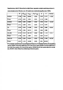
Abstract The purpose of this project was to study relationship among air pollutants, SO2, NO2 and PM10, then created a linear regression equation for predicting SO2 in the different 3 periods, January-April, May-August and SeptemberDecember. The project results found that the 3 linear regression equations, (Jan -Apr) = 2.02 + 0.0871 NO2(Jan-Apr) with the minimum percentage SO 2 of error in April of 21.9818 and the adjusted coefficient of determination of (May - Aug) =1.84 + 0.0491 PM10(May-Aug) 35.8 for the first period, SO 2
with the minimum percentage of error in May of 4.1667 and the adjusted coefficient of determination of 29 for the second period and (Sep - Dec) =4.06 – 0.0922 NO2(Sep-Dec) with the minimum percentage SO 2
of error in November of 0.000 and the adjusted coefficient of determination of 56.7 for the last period. Mathematics Subject Classification: 62J05 Keywords: multicollinearity, variance inflation factor, best subset method
INTRODUCTION Thailand has been classified by the United Nation as a developing country because it is expanding numerous manufactures caused to various pollution problems [1]. Therefore, it is particularly at the east of Thailand is facing pollution issues due to a lot of industrial estates. Chonburi, one of the eastern provinces contains many industrial factories confronting with diverse air pollution problem. It effects to health
2166
J. Mekparyup et al
problems and environmental issues. The Sulfur dioxide (SO2), Nitrogen dioxide (NO2) and Particulate matter smaller than 10 microns (PM10) are most of all common pollutants from industrial sources affected to the respiratory system especially SO2 [2][3][4]. This project proposed to estimate SO2 for planning in order to reduce the affectation to the community and the environment.
MATERIALS AND METHODS Air Quality and Noise Management Bureau, Polluation Control Department, Thialand provided SO2, NO2 and PM10 since 1996 to 2013. The four steps of this project were as follows.
1. STUDYING THE RELATIONASHIP AMONG SO2, NO2 AND PM10 The correlation coefficient (R) of each pair of SO 2, NO2 and PM10 was calculated to study the relationship among SO2, NO2 and PM10,
2. BUILDING THE MULTIPLE LINEAR REGRESSION EQUATION OF SO2 Data was separated by 3 different periods which were January to April, May to August and September to December then the multiple linear regression (MLR) equations to estimate monthly SO2 were generated [2][3][4] following Equation 1, 2 and 3 consequently.
SO2 (Jan-Apr) 01 11NO2 (Jan-Apr) 21PM10 (Jan-Apr) SO2 (Jan-Apr)
(1)
SO2 (May-Aug) 01 11NO2 (May-Aug) 21PM10 (May-Aug) SO2 (May-Aug) (2)
SO2 (Sep-Dec) 01 11NO2 (Sep-Dec) 21PM10 (Sep-Dec) SO2 (Sep-Dec)
(3)
The best subset method was used to consider appropriateness of MLR equation by Mallow C-p value, standard error of estimation (S) and the adjusted coefficient of 2 determination ( Radj ).
3. CHECKING ASSUMPTIONS OF MLR After received the best fitted MLR equation, the assumptions of MLR was testified. There are four assumptions to be checked; (I) normality of the error distribution using Anderson-Darling statistic (AD) by [5]; (II) independence of the errors using DurbinWatson statistic (DW) by [6]; (III) homoscedasticity (constant variance) of the errors using Breusch-Pagan statistic (BP) by [7]; (IV) multicollinearity among predictor variables using Variance Inflation Factor (VIF) [8].
Predicting SO2 with Multiple Linear Regression Equation in Chonburi
2167
4. DETERMINING THE APPROPRIATE OF MLR After testing all assumptions, the observation value (OBS) and predicted value (PRE) were calculated to determine the appropriateness of the three MLR equations with the percentage of error (PE) as of Equation 4.
PE
OBS PRE 100% OBS
(4)
RESULTS AND DISCUSSION Calculating correlations coefficient (R) in each period, the first period, the significant positive correlations between SO2(Jan-Apr) and NO2(Jan-Apr) was found with R=0.611 (p-value=0.000), the second period, significant positive correlation between SO2(May-Aug) and NO2(May-Aug) were displayed with R=0.550 (p-value=0.000) and the last period, the significant positive correlations between SO 2(Sep-Dec) and NO2(Sep-Dec) was recognized with R=0.406 (p-value=0.001). All above results were the same period in agreement of the previous studies [2][3][4]. Fitting MLR equation in each period using the best subsets method, the first period, (Jan-Apr) = 2.02 + 0.0871 NO2(Jan-Apr) with the the MLR equation was SO 2
2 minimum Mallow C-p= 1.1, S=1.2990 and Radj =10.2, the second period, the MLR
(May-Aug) = 1.84 + 0.0491 PM10(May-Aug) with the minimum equation was SO 2 2 Mallow C-p= 1.0, S=0.82894 and Radj =23.3 and the last period, the MLR equation
(Sep-Dec) = 4.06 + 0.0922 NO2(Sep-Dec) + 0.0343 PM10(Sep-Dec) with the was SO 2 2 minimum Mallow C-p=3.0, S=1.1094 and Radj =14.9.
Checking assumptions of all fitted MLR equations, (I) ADs were determined for testing of normality in each period and the results were satisfied with AD=0.261 (pvalue=0.963), AD=0.597 (p-value=0.116) and AD=0.306 (p-value=0.557). (II) DWs were examined for testing of independence of errors in each period and found that DW=1.7478 (DL=1.475), DW=1.67023 (DL=1.549) and DW=1.67401 (DL=1.536) so the errors were independent for all periods. (III) BPs were illustrated for testing of homoscedasticity of error variation in each period and showed BP=0.2648 (pvalue=0.6068), BP=1.3363 (p-value=0.2476) and BP=3.8669 (p-value=0.049247) so the error variances were constant. (IV) VIFs were calculated for testing of multicollinearity and all values in each period were less than 5 then there was no relationship among independent variables in all MLR equations [9]. Determining the appropriateness of all MLR equations by PE value following Equation 4, the results were displayed in Table 1. The maximum and minimum PE value was found with 80.01% in January and 0.00% in November consequently.
2168
J. Mekparyup et al Table 1. The percentage of error (PE)
Month PRE OBS PE
Jan 1.80 1 80.01
Feb 2.12 3 29.22
Mar 3.66 4 14.58
Apr 3.66 3 21.98
May 1.92 2 4.17
Jun 2.14 2 6.94
Jul 2.47 3 17.59
Aug 2.47 2 23.61
Sep 1.79 2 10.71
Oct 1.64 1 64.29
Nov 2.00 2 0.00
Dec 1.57 2 21.43
DISCUSSION The data was separated in the different 3 periods, January-April, May-August and September-December. In each period, NO2 and PM10 were considered to generate the 2 MLR equation for predicting SO2 by NO2 with S=1.2990 and Radj =10.2 for the first, 2 PM10 with S=0.82894 and Radj =23.3 for the second and both NO2 and PM10 with 2 S=1.1094 and Radj =14.9for the last. The accuracy of prediction was testified by the
percentage of error (PE) and the results found perfectly well with PE=0.00% in November.
ACKNOWLEDGEMENT We are grateful to Air Quality and Noise Management Bureau, Polluation Control Department, Thialand for kindly providing all data.
REFERENCES [1]
United Nation, (2014). Country classification. Retrieved July 4, 2014, from the United nations. Web site : http//www.un.org/en/development/desa/policy/wesp/wesp-current/ 2012County-class.pdf [2] Wheeler, A. J., Smith-Doiron, M., Xu, X., Gilbert, N. L., & Brook, J. R. (2008). Intra-urban variability of air pollution in Windsor, Ontario— measurement and modeling for human exposure assessment. Environmental Research, 106(1), 7-16. [3] Kar, S., & Mukherjee, P. (2012). Studies on Interrelations among SO2, NO2 and PM10 Concentrations and Their Predictions in Ambient Air in Kolkata.Open Journal of Air Pollution, 1, 42. [4] Kavuri, N. C., Paul, K. K., & Roy, N. (2012, December). Regression modeling of gaseous air pollutants and meteorological parameters in a steel city, Rourkela. In 2nd International Science Congress (ISC-2012), 8th-9th December 2012, Mathura, UP, India. [5] Lewis, P.A.W., 1961, ―Distribution of the Anderson-Darling Statistic,‖ The Annals of Mathematical Statistics, 32(4), 1118-1124.
Predicting SO2 with Multiple Linear Regression Equation in Chonburi [6] [7] [8] [9]
2169
Durbin, J., & Watson, G.S., 1951, ―Testing for Serial Correlation in Least Squares Regression II,‖ Biometrika, 38(2), 159-177. Breusch T.S., & Pagan, A.R., ―A Simple Test for heteroscedasticity and Random Coefficient Variation,‖ Econometrica, 47(5), 1287-1294. O’brien, R. M. (2007). A caution regarding rules of thumb for variance inflation factors. Quality & Quantity, 41(5), 673-690. Kutner, M.H., Christopher, J.N., & Neter, J., 1996, ―Applied liner regression models, 4th ed,‖ McGraw-Hill/Irwin , USA.
2170
J. Mekparyup et al