rapidly-exploring random tree (RRT) and long short-term memory (LSTM) net- ... uration space by the RRT method, a convolutional autoencoder and LSTM ...
Robot Path Planning by LSTM Network Under Changing Environment Masaya INOUE, Takahiro YAMASHITA, and Takeshi NISHIDA Kyushu Institute of Technology, 1-1 Sensui, Tobata, Kitakyushu, Fukuoka 804–8550, Japan
Abstract. We propose a novel robot path planning method that combines the rapidly-exploring random tree (RRT) and long short-term memory (LSTM) network. In this method, numerous and good paths are generated in the robot configuration space by the RRT method, a convolutional autoencoder and LSTM combination network is trained by them. The proposed method overcomes the difficulty of general methods with neural networks, i.e., “the acquisition of a large amount of training data.” Moreover, the difficulty of general random based methods, i.e., “the reproducible path generation” is resolved with high-speed.
1 Introduction Path planning is an important function for executing autonomous moving robots, and many path planning methods that satisfy various constraints, such as avoiding obstacles and energy efficiency, have been proposed. There are many random sampling algorithms widely used for robot path planning, such as the probabilistic roadmap [1], rapidly-exploring random tree (RRT) [2], and their improved algorithms. These methods are used for connecting nodes to create a path and create a strong feature so that the path can always be found under the condition that the starting point and goal point can be connected. Moreover, in situations where obstacles or other factors exist in the target area, or when the environment dynamically changes, it is difficult to set nodes to be prescribed in space. Therefore, it is known that these methods are more advantageous in such situations compared to Dijkstra’s algorithm and A* method [3] that use fixed nodes. However, since these algorithms use random numbers, some problems occur, such as fluctuations of the found path for each search time and finding a redundant path when the search time is not sufficient. On the other hand, path planning methods by machine learning such as methods using a neural network (NN) [4] and deep Q-network combining reinforcement learning [5] have been proposed. Although these methods require large amounts of learning beforehand, they can generate paths at high speed after learning. In addition, unlike the abovementioned methods, the same path is generated for the same starting point and goal point. Owing to the generalization ability of NN, path generation is possible even for conditions not used during learning. However, these methods cannot positively take into account the robot’s physicality as prior knowledge, and trial and error is required to acquire a large amount of training data for learning. It is often impossible to perform many trial and error processes on site.
Therefore, we propose a new path planning method that combines the random sampling method and NN method to overcome “the fluctuation and redundancy of found path” with the random sampling algorithm and “the acquisition of a large amount of training datasets” for the NN method. In the proposed method, a large amount of highquality paths are generated by RRT in the configuration space by considering the robot’s physicality and environment, and learning by the NN is executed using these datasets. After learning, the NN can generate a high-quality path quickly and stably. This network also develops generalization ability.
2 Problem setting First, let C be the configuration space of a robot. In this study, to simplify the analysis we set C ⊂ IR2 and the region is set as { C=
} p ≜ [p1 p2 ] p1l ≤ p1 ≤ p1u , p2l ≤ p2 ≤ p2u , T
(1)
where p1l , p1u , p2l , and p2u are constant. The starting points ps and the goal points pg of the paths are generated using random numbers in the specific regions. The regions of Cs ⊂ C and Cg ⊂ C are set as follows: } Cs = ps ≜ [p1s p2s ] p1sl ≤ p1s ≤ p1su , p2sl ≤ p2s ≤ p2su , { } T Cg = pg ≜ [p1g p2g ] p1gl ≤ p1g ≤ p1gu , p2gl ≤ p2g ≤ p2gu . {
T
We consider the problem of generating a path that connects arbitrarily set starting points ps ∈ Cs and goal points pg ∈ Cg without colliding with obstacles. Next, the path generated using the starting point and goal point pair is expressed as follows: { } (n)
(n)
(n) (n) P (n) ≜ p(n) , s , p1 , · · · , pe , · · · , pE , pg
(2)
where n = 1, · · · , N represents the path number; m = 1, · · · , E is the node number; (n) and pe ∈ C is a node of the path. The sum of the Euclidean distances between the nodes is called the total length of the path. In this research, we consider the problem based on C ⊂ IR2 ; hence, we describe the configuration space as an image with obstacles. The image is represented as matrix I (r) ∈ IRA×B composed of pixels, where r = 1, · · · , R is the index of the image, and A and B are the number of pixels of the height and width of the image, respectively. The obstacle area is represented by setting the value of matrix elements as 1, and there are no obstacles in Cs and Cg . Also, the value of matrix elements representing the region where the obstacle does not exist is 0. The path P (n) used for training must be set so that there are no obstacles on the node and the line segment connecting them.
Path generation network LSTM section Next time input..
Fll connected Copy Flattening Convolution
Output layer
....
Given: CAE section
....
.... ....
{ {
Input layer
Fig. 1. Overview of the proposed network. This shows signal flow in the recalling phase.
3 Proposed Path Planning Method 3.1 Architecture of Proposed Network The proposed network for path generation consists of the convolutional autoencoder (CAE) [7] and long short-term memory (LSTM) network [8]. The overview is shown in Fig. 1. The CAE section is integrated into the LSTM for feeding the environmental information, and the LSTM section executes the path generation. The proposed method has four phases as follows: 1. Training of the CAE section (CAE training phase). 2. Generating training data sets using trained CAE and RRT (Training data generating phase). 3. Path training by LSTM network (LSTM training phase). 4. Generating the new path (Recalling phase). This process is illustrated in Fig.2.
1.CAE Training phase
data 2. Training generating phase Paths generated by RRT
4.Recalling phase
3.LSTM Training phase Training data
Loss Weight
update
RRT algorithm
New path
Weight update
LSTM network model
LSTM network model
CAE Conv
Random environmental image
New fine path
Loss
Deconv
Defined MAP
Start and goal points pairs are randomly generated
New start and goal points
Conv
Fig. 2. Flow of the phases of the proposed method.
Conv Any MAP
3.2 CAE Section Structure of CAE Section In this section, the information of obstacles are extracted from I (r) and the size is compressed by the CAE. Then, the output from the CAE is integrated with the path information in the input layer of the LSTM section. By compressing the image I (r) , the size of the LSTM section is reduced. Furthermore, by inputting information on the environment to the LSTM, it becomes possible to generate a path suitable for various environments. If there is no CAE section, the LSTM only learns the statistics of the paths without information on obstacles and avoids it. In this a case, it is impossible to acquire latent knowledge that obstacles must be avoided. The CAE section is an LC layered convolutional NN. Convolution processing is known to be very effective in image recognition. The convolution in the lC -th layer is (lC −1) executed against the element zabd of the output tensor ZCAE ∈ IRC×V ×Q using an V ×Q×C×D element hvqcd of the filter set H ∈ IR
(lC ) uabd
=
Q C ∑ V ∑ ∑
(l −1)
(l )
(l )
C C C zsa+v,sb+q,c hvqcd + babd
(3)
c=1 v=1 q=1
( ) (lC ) (lC ) zabd = η (lC ) uabd
(4)
where V and Q are the sizes in the horizontal and vertical axis direction of the filter, respectively; c = 1, · · · , C represents the channel number of input tensor; d = 1, · · · , D is the number of filters; s is the pixel width scanned by the filter; babd is a bias; and η (lC ) (·) is called the activation function. The output tensor of the first layer corresponds to I. In addition, each element z corresponds to each pixel. During training, restoration is performed using an LC layered deconvolution layer, and the error backpropagation method is applied to the error between the restored image and original image. The deconvolution layer is the layer that performs convolution processing after padding target matrix components with arbitrary values [10]. It also has the function of restoring the compressed tensor by convolution layer. CAE Training Phase The CAE section is trained using environmental datasets with the following procedure: (1) Using randomly-positioned obstacles, a large amount of environmental images I (r) are generated. (2) The images I (r) are divided into mini-batch sets, and CAE training is executed using these. (3) Learning is aborted after sufficiently repeating (2). Training Data Generating Phase The training dataset for LSTM section is generated with the following procedure: (rn)
(1) Give I (r) (r = 1, · · · , R) and N sets of start ps (n = 1, · · · , N ) for each image.
(rn)
∈ Cs and goal pg
∈ Cg
(rn)
(rn)
(2) Generate paths P (rn) using ps and pg in I (r) by applying RRT. (3) Modify the generated paths by the trajectory refinement method. (4) Extract high-quality paths based on the number of nodes E. It should be noted that in (4), the mode value of the number of nodes of generated paths is found; paths with number of nodes that deviate from this value are deleted. With these procedures, various paths for environmental images containing various obstacles (r) are generated. Then, the image information ZCAE compressed by the CAE and path (rn) P are combined to become the training datasets of the LSTM. 3.3 LSTM Section Let us assume an LSTM network with LL layers. There are two input layers and hidden layers that receive outputs from them in this network, they are integrated in the upper hidden layer and connected to the output layer. Specifically, in the simulation described later, the input of the input layer that accepts the CAE output is called xkC ∈ IR108 , while the input of the input layer that accepts information on the route is called xkL ∈ IR4 [ ]T (r) xkC = zCAE , xkL = y (k−1)T pTg , y k = pk , (r)
(5)
(r)
where zCAE is a flattened vector of ZCAE output of the CAE section, y 0 = ps , and k represents the recalling step corresponding to node number. When xk is input into the LSTM network, the network recalls the next node of path y k . The number of cells in the input layers are 108 and 4, and they are fully connected to the corresponding hidden layers. The number of cells in each hidden layer is larger than the number of cells in the input layers (e.g., 120). The output of the hidden layers are integrated into the next hidden layer. LSTM Network The input and output vectors of the lL -th layer at time k are represented by [ ]T (lL ),k (lL ),k L ),k , u(lL ),k ≜ u(l · · · u · · · u 1 j J [ ]T z (lL ),k ≜ z1(lL ),k · · · zj(lL ),k · · · zJ(lL ),k
(6) (7)
where j is the unit number, J is the total number of units, and J is not common to all layers. The input vector is xk = u(1),k in the input layer, and the output vector is y k = z (LL ),k in the output layer. The unit number and total number of units of the (lL − 1)-th layer are represented by j − and J − , respectively. The input propagation weight from − the (lL − 1)-th layer to the l-th layer is represented by W (lL ) ∈ RJ×J . The recurrent (lL ) weight in the lL -th layer (lL = 2, · · · , LL − 1) is represented by R ∈ RJ×J . The (l) bias is represented by b , and each component is represented by w, r, and b. Here, j ′ is an arbitrary unit number corresponding to the output signal of the time k − 1 of the lL -th layer The components of u(lL ),k are given by
−
(l ),k uj L
=
J ∑
(l ) (l −1),k
wjjL− zj −L
+
J ∑
(l ) (l),k−1
rjjL′ zj ′ +
(l )
+ bj L .
(8)
j′
j−
The elements of the output vector of the l-th layer are represented by ( ) (l ),k (l ),k zj L = η (lL ) uj L .
(9)
To summarize the discussion above, the output of the l-th layer is represented as ( ) z (lL ),k = η (lL ) W (lL ) z (lL −1),k + R(lL ) z (lL ),k−1 + b(lL ) ,
(10)
and the output of the output layer is represented as ( ) y k = η (LL ) W (LL ) z (LL −1),k .
(11)
LSTM Unit The LSTM network is constructed by LSTM units [9], and the following calculation is executed for each unit. First, the forget gate opening ratio of the d-th unit is calculated as ( ) fdk = σ wdf g xk + rdf g z (k−1) + bf g , (12) where σ(·) is the logistic sigmoid function, wdf g is a weight vector corresponding to the input vector xk from the previous layer, rdf g is a weight vector corresponding to the input vector z k−1 from previous time, and bf g is a bias. Next, the opening ratio of the input gate is calculated as ( ) ikj = σ wjig xk + rjig z (k−1) + big . (13)
ForgetGate
MemoryCell
InputGate OutputGate
�summing point
�logistic sigmoid
�multiply point
�sigmoid
Fig. 3. Structure of a LSTM unit.
The signal through the input gate is
( ) Mjk = fjk · Mjk−1 + ikj · tanh wjz xk + rjz z (k−1) + bz .
(14)
This value is transmitted as the internal state of the unit at the next time. Then, the opening ratio of the output gate is calculated as ( ) okj = σ wjog xk + rjog z (k−1) + bog , (15) and the output value zjk is derived as zjk = okj · tanh(Mjk ).
(16)
LSTM Training Phase The LSTM network is trained using the path dataset as follows: (1) Shuffle the datasets {I (r) , P (rn) } and divide them into mini-batch sets. (2) Execute the following processes on the first mini-batch. 1. xk is constructed from the dataset and input into tge LSTM at time k. 2. y k is recalled by forward propagation of xk . 3. Distance between y k and P (rn) is accumulated as recalling error. 4. Construct xk+1 using y k , time step is replaced k := k + 1, and return to 2. 5. Loop until the final time. (3) Modify connection weights in the network using backpropagation through time method [8]. (4) Execute the processing of (2) and (3) for the next mini-batch, and execute all minibatches as well (This is called 1 epoch). (5) Repeat processes (1)–(4) and execute a sufficient number of epochs. 3.4 Generating the new path When a combination of an environmental image and a desired starting point and goal point is input into the network where learning has been completed, a path is generated. The network continues to generate nodes y k until it approaches the goal point. Stop the path generation when it approaches the goal point beyond a certain threshold and combine it with the goal point.
Obstacle
Obstacle
Obstacle
(a) Two-dimensional region including obstacles.
(b) Examples of environmental images.
Fig. 4. Configuration space C or environmental image I (r) .
Fig. 5. Results of generalization test of CAE.
4 Simulation 4.1 Conditions Examples of configuration space C or environmental image I (r) supposed in experiments are shown in fig. 4. The vertical and horizontal sizes of this image were set as p1 ∈ [−1, 1] and p2 ∈ [−1, 1], respectively. 4.2 Training Training of CAE Table1 shows the parameters of the constructed CAE section. With the CAE section, the environmental information I (r) ∈ IR100×100 was compressed to (r) ZCAE (A = 6, B = 6, D = 3) by three convolution processes. The training of the CAE section was executed by restoring the compressed signal in the deconvolution layer and applying the error backpropagation method to the error from the original image. In order to confirm the generalization ability of the CAE section after the training phase, the environmental image which was not used for learning was restored after compression. The results of the generalization test, shown in Fig. 5, demonstrate that the CAE section acquired the ability to extract environmental features. Training Data Generation and Training of LSTM Ten types (i.e., r = 10) of environmental images with different obstacle arrangements were prepared. We also set Table 1. Parameters of the CAE section. Setting items Size of environmental image I (r) ∈ IRA×B Number of convolutional layers LC Number of filters in each layer Number of stride sizes in each layer s Filter size (V × Q) Activation function η(·). Error function Mini-batch size Initial weights Initial bias Learning rate adjustment
Detail A = B = 100 3 12, 6, 3 1, 3, 5 V =Q=5 Rectifier function Mean squared error 200 Random number in [−0.1, 0.1) None Adam [12]
Table 2. Parameters of the LSTM network. Setting items Input dimension Output dimension Number of hidden layers Number of units in one hidden layer Activation function of output layer Error function Mini-batch size Initial weights Initial bias Learning rate adjustment
Detail 108(CAE), 4 2 2 120 Identity function Mean squared error 200 Random [−0.1, 0.1) None Adam [12]
p1sl = −1.0, p1su = −0.5, p2sl = 0.5, and p2su = 1.0 to set Cs , and p1gl = 0.5, p1gu = 1.0, p2gl = −1.0, and p2gu = −0.5 to set Cg . Next, we sampled n = 3500 combinations of start and goal points from Cs and Cg , and generated paths P (rn) using RRT implemented in the Open Motion Planning Library [11]. We carried out processing to refine the generated paths using the path pruning method, shortcut method [13], and B-spline method [14]. Through these procedures, we constructed the training dataset {I (r) , P (rn) |r = 10, n = 3500}. The main parameters of the LSTM section are listed in Table 2. 4.3 Recalling of Path Path generation in trained environment The network was trained in 10 environments, and the path generation ability of the trained network was investigated against arbitrary chosen starting and goal points in the trained environment. Examples of generated paths are shown in Fig.6. A route was generated by preparing 10,000 random pairs of starting points and goal points for each environment. Table 3 shows the success
Map1
Map2
Map3
Map4
Map5
Map6
Map7
Map8
Map9
Map10
Fig. 6. Examples of the generated paths in trained environments. The symbol ♢ represents the starting point, and the symbol⋆ represents the goal point.
Table 3. Success rates of path generation in trained environment. environment
Map1 Map2 Map3 Map4 Map5 Map6 Map7 Map8 Map9 Map10
Success rate [%] 98.23 99.99 99.61 70.13 99.97 98.31 99.32 100 94.38 99.46
rates of path generation without collision with obstacles. The success rates were over 98% in 8 out of 10 environments. Path generation in unknown environment The path generation ability of the trained network was investigated against arbitrary starting and goal points in an unknown environment. Examples of generated paths are shown in Fig.7. In the unknown environment, similar to the learned environment, the success rate was relatively high and path generation often failed when the environment was significantly different from the trained environment. Therefore, in order to verify the generalization ability of the trained network, the positions of all the obstacles in a specific trained environment were randomly fluctuated, and the change in the success rate of route generation was observed. The vertical and horizontal positions of all the obstacles in the environment shown in map 1 of Fig.6 were fluctuated from ±0.01 to ±0.2 [m] randomly and individually. The results shown in Fig.8 demonstrate that sufficiently high performance or generalization ability can be expected if fluctuations in the position of the obstacle are within 10%. It is found from these results that when the given environment is similar to the trained data set, the network realizes high path generation capability. Namely, since the network outputs the appropriate number of nodes and paths based on the training data set, it will be possible to improve the generalization ability by extending the training data set.
5 Conclusion The proposed method has the following advantages: (1) In trained environments, paths can be generated without colliding with obstacles even if the starting and goal points change. (2) Even for unknown environments similar to trained environments, the method has the ability to generalize path generation. (3) In the composition of the dataset, path selection based on arbitrary evaluation index is possible. (4) It is possible to prevent the generation of poor quality or redundant trajectory caused by the trajectory generation method such as RRT. (5) The generated path does not fluctuate unlike with methods based on random numbers. (6) Path generation after training can be done quickly. (7) It is possible to configure the proposed method as hardware that operates at low power and high speed. We proposed a method to construct an LSTM network that recalls the
(a) Examples of success.
(b) Examples of failure.
Fig. 7. Examples of the generated paths in unknown environments.
Success rate [%]
100
98.23
98.05
94.83
92.10 76.00
75
54.49
50 26.15
25 0 0
0.01
0.03
0.05
0.07
0.1
0.2
Perturbation length [m] Fig. 8. Relationship between magnitude of environmental change and collision rate.
path of a robot by training with a large number of paths generated by RRT. The simulation results confirm that the proposed network achieves high learning and generalization abilities.
References 1. Kavraki, L. E., Svestka, P., Latombe, J. -C., and Overmars, M. H., “Probabilistic roadmaps for path planning in high-dimensional configuration spaces,” IEEE Trans. on Robotics and Automation, 12.4, 566–580 (1996) 2. LaValle, S. M., Kuffner, J. J., “Rapidly-exploring random trees: Progress and prospects,” Algorithmic and Computational Robotics: New Directions, Wellesley, 293–308 (2001) 3. Choset, H., Lynch, K., Hutchinson, S., Kantor, G., Burgard, W., Kavraki, L., Thrun, S., “Principles of Robot Motion: Theory, Algorithms, and Implementations,” Cambridge: MIT Press (2005) 4. Yang, Simon X., and Max Meng. “An efficient neural network approach to dynamic robot motion planning,” Neural Networks, 13.2, 143–148 (2000) 5. Gu, Shixiang, et al. “Deep Reinforcement Learning for Robotic Manipulation with Asynchronous Off-Policy Updates.” arXiv preprint arXiv:1610.00633 (2016) 6. Bin, N., Xiong, C., Liming, Z., Wendong, X., “Recurrent neural network for robot path planning,” Parallel and Distributed Computing: Applications and Technologies. Springer Berlin Heidelberg, 188–191 (2004) 7. Masci, J., Meier, U., Cirean, D., Schmidhuber, J. , “Stacked convolutional auto-encoders for hierarchical feature extraction”, Artificial Neural Networks and Machine LearningICANN 2011, 52–59 (2011) 8. Ilya, S., Training recurrent neural networks, University of Toronto (2013) 9. Gers, F. A., Schmidhuber, J., and Cummins, F., “Learning to forget: Continual prediction with LSTM,” Neural computation, 12.10, 2451–2471, (2000) 10. Zeiler, M. D., Krishnan, D., Taylor, G. W., Fergus, R. , “Deconvolutional networks”, In Computer Vision and Pattern Recognition , 2010 IEEE Conference on , 2528–2535 (2010) 11. Sucan, Ioan A., Mark Moll, and Lydia E. Kavraki. “The open motion planning library.” IEEE Robotics & Automation Magazine 19.4, 72–82 (2012) 12. Diederik, D., Ba, J., “Adam: A method for stochastic optimization,” arXiv preprint, arXiv:1412.6980 (2014) 13. Harada, K. “Optimization in Robot Motion Planning,” JRSJ, 32.6, 508–511 (2014) 14. Harada, K., Hattori, S., Hirukawa, H., Morisawa, M., Kajita, S., Yoshida, E., “Two-stage time-parametrized gait planning for humanoid robots,” IEEE/ASME Transactions on Mechatronics, 15.5, 694–703 (2010)