Dynamic Integration of Multiple Data Mining Techniques in a ...

Header for SPIE use

Dynamic Integration of Multiple Data Mining Techniques in a Knowledge Discovery Management System Seppo Puuronen*a, Vagan Terziyanb, Artyom Kasatonovb, Alexey Tsymbalb a

Dept. of Comp. Sc. & Inf. Systems, Univ. of Jyvaskyla, P.O.Box 35, FIN-40351 Jyvaskyla, Finland bDept.

of AI & Inf. Systems, State Technical Univ. of Radioelectronics/Kharkov/Ukraine ABSTRACT

One of the most important directions in improvement of the data-mining and knowledge discovery methods is the integration of the multiple classification techniques based on ensembles of classifiers. An integration technique should solve the problem of estimation and selection of the most appropriate component classifiers for an ensemble. We discuss an advanced dynamic integration of multiple classifiers as one possible variation of the stacked generalization method using the assumption that each component classifier is best inside certain areas of the application domain. Initially we have a number of cases represented in some space. For each of these cases we know an appropriate outcome. The problem is how to derive an outcome for every new case in the same space. We have also a set of classifiers and each of them can calculate the outcome in every point (case) of the space. We assume that for each case there exists an optimal classifier in our set that can derive the outcome more precisely than using other classifiers. Thus first we have developed a learning technique to derive the “competence areas” for all classifiers in our space of cases. In the learning phase a performance matrix of each component classifier is derived and then used in the application phase to predict performances of each component classifier with new instances. Method was evaluated on three data sets taken from the UCI machine learning repository, with which well-known classifier integration methods are proven to perform badly. Results show that the dynamic integration method often significantly outperforms other integration methods. Keywords: Data mining, supervised learning, ensemble of classifiers, dynamic integration, stacked generalization

1. INTRODUCTION Data mining is the process of finding previously unknown and potentially interesting patterns and relations in large 6 databases . Currently electronic data repositories are growing quickly and contain huge amount of data from commercial, scientific, and other domain areas. The capabilities for collecting and storing all kinds of data totally exceed the abilities to analyze, summarize, and extract knowledge from this data. Numerous data mining methods have recently been developed to extract knowledge from large databases. In many cases it is necessary to solve the problem of evaluation and selection of the most appropriate data-mining method or a group of the most appropriate methods. Often the method selection is done statically without analyzing each particular instance. If the method selection is done dynamically taking into account characteristics of each instance, then data mining usually gives better results. During the past several years, in a variety of application domains, researchers try to combine efforts to learn how to create 5 and combine an ensemble of classifiers. For example, integrating multiple classifiers has been shown to be one of the four most important directions in machine learning research. The main discovery is that ensembles are often much more accurate 17 than the individual classifiers. The two advantages that can be reached through combining classifiers are shown : (1) the possibility that by combining a set of simple classifiers, we may be able to perform classification better than with any sophisticated classifier alone, and (2) the accuracy of a sophisticated classifier may be increased by combining its predictions with those made by an unsophisticated classifier.

*

Correspondence: Email: [email protected]; WWW: http://www.cs.jyu.fi; Telephone: 358 14 603 028; Fax: 358 14 603 011

We use an assumption that each data mining method has its competence area inside the application domain. The problem is then to try to estimate these competence areas in a way that helps the dynamic integration of methods. From this point of view data mining with a set of available methods has much in common with the multiple expertise problem. Both problems 18 solve the task of receiving knowledge from several sources and have similar methods of their decision. Previously we have suggested a voting-type technique and recursive statistical analysis to handle knowledge obtained from multiple medical 19 experts. We also presented a meta-statistical tool to manage different statistical techniques used in knowledge acquisition. In this paper we apply this kind of thinking to the problem of dynamic integration of classifiers. Classification is a typical data mining task consisting in explaining and predicting the value of some attribute of the data given a collection of tuples 2 with known attribute values . We discuss the problem of integrating multiple classifiers and consider basic approaches suggested by various researchers recently. Then in the third chapter, we present the dynamic classifier integration approach that uses classification error estimates. In the next chapter, we present the results of the experiments. We conclude with a summary of obtained results and with further research topics.

2. INTEGRATING MULTIPLE CLASSIFIERS: RELATED WORK Integrating multiple classifiers to improve classification has been an area of much research in machine learning and neural networks. Different approaches to integrate the multiple classifiers and their applications have been 2,5,7,9,10,11,14,16-21 considered . Integrating a set of classifiers has been shown to yield accuracy higher than the most accurate component classifier for different real-world tasks. The challenge of the problem considered is to decide which classifiers to rely on for prediction or how to combine results of component classifiers. The problem of integrating multiple classifiers can be defined as follows. Let us suppose that a training set T and a set of classifiers C are given. The training set T is: (x i , yi ), i  1,..., n , where n is the number of training instances, xi is the i-th



 



training instance presented as a vector of attributes x j , j  1,..., l (values of attributes are numeric, nominal, or symbolic),



and yi  c1 ,..., ck

 is the actual class of the i-th instance, where k is the total number of classes.

The set of classifiers C is:

C ,..., C , 1

m

where m is the number of available classifiers (we call them component

classifiers). Each component classifier is either derived using some learning algorithm or hand-crafted (non-learning) classifier constructed using some heuristic knowledge. A new instance x* is an assignment of values to the vector of attributes x j . The task of integrating classifiers is to classify the new instance using the given set C of classifiers.

 

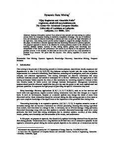
Recently two basic approaches are used to integrate multiple classifiers. One considers combining the results of component classifiers, while the other considers selection of the best classifier for data mining. Several effective methods have been proposed which combine results of component classifiers. One of the most popular and simplest methods of combining 10 classifiers is simple voting (also called majority voting and Select All Majority, SAM) . In voting, the prediction of each component classifier is an equally weighted vote for that particular prediction. The prediction with most votes is selected. Ties are broken arbitrarily. There are also more sophisticated methods that combine classifiers. These include the stacking 21 (stacked generalization) architecture , SCANN method based on the correspondence analysis and the nearest neighbor 11 17 procedure , combining minimal nearest neighbor classifiers within the stacked generalization framework , different versions of resampling (boosting, bagging, and cross-validated resampling) that use one learning algorithm to train different 5,16 classifiers on subsamples of the training set and then simple voting to combine those classifiers . Two effective classifiers' 2 combining strategies are based on stacked generalization and called an arbiter and combiner . Hierarchical classifier 2 combination was also considered. Experimental results showed that the hierarchical combination approach was able to sustain the same level of accuracy as a global classifier trained on the entire data set distributed among a number of sites. 21 Many combining approaches are based on the stacked generalization architecture considered by Wolpert . Stacked generalization is the most widely used and studied model for classifier combination. A basic scheme of this architecture is presented in Fig. 1.

Final Prediction M(C1(x*),..., Cm(x*) ) Combining (Meta-Level) Classifier M

Meta-Level Training Set

(C (x

M

1

Component Predictions Ci(x*) Component Classifiers Ci

C1

C1(x*)



),..., Cm ( x j ), y j )

Cm(x*)

C2(x*)

C2

j

...

Cm

Example x* Fig. 1. Basic form of the stacked generalization architecture

The most basic form of the stacked generalization layered architecture consists of a set of component classifiers

C  C1 ,..., Cm  that form the first layer, and of a single combining classifier M that forms the second layer. When a new

instance x* is classified, then first, each of the component classifiers Ci is launched to obtain its prediction of the instance’s class Ci(x*). Then the combining classifier uses the component predictions to yield a prediction for the entire composite classifier M(C1(x*),..., Cm(x*) ). The composite classifier is created in two phases: first, the component classifiers Ci are





created and second, the combining classifier is trained using predictions of component classifiers Ci (x j ) and the training set T

17,21

.

Even such widely used architecture for classifier combination, as stacked generalization, has still many open questions. For example, there are currently no strict rules saying which component classifiers should be used, what features to use to form the meta-level training space for combining classifier, and what combining classifier one should use to obtain an accurate composite classifier. Different combining algorithms have been considered by various researchers. For example, the classic 16 17 boosting uses simple voting , Skalak discusses ID3 for combining nearest neighbor classifiers , and the nearest neighbor 11 classification is proposed to make search in the space of correspondence analysis results (not directly on the predictions). Several effective approaches have recently also been proposed for selection of the best classifier. One of the most popular 10 and simplest approaches for classifier selection is CVM (Cross-Validation Majority) . In CVM, the cross-validation accuracy for each classifier is estimated with the training data, and a classifier with the highest accuracy is selected. In the case of ties, the voting is used to select among classifiers with the best accuracy. Some more sophisticated selection approaches include, for example, estimating the local accuracy of component classifiers by considering errors made in 10 instances with similar predictions of component classifiers (instances of the same response pattern) , learning meta-level classifiers (“referees”) that predict whether the component classifiers are correct or not for new instances (each “referee” is a 14 C4.5 tree that recognizes two classes) . Previously we have considered an application of classifier selection to medical 18,19,20 diagnostics . It uses predicting the local accuracy of component classifiers by analyzing the accuracy in near-by instances. This paper considers an improvement of the classifier selection approach. The set of known classifier selection methods can be partitioned into two subsets of static and dynamic selection. The static approaches propose one “best” method for the whole data space, while selection by dynamic approaches depends on each new instance analyzed. CVM is an example of static approach, while the other selection methods above and the one proposed in this paper are dynamic.

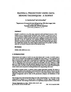
3. DYNAMIC INTEGRATION OF CLASSIFIERS USING META-LEARNING In this chapter we consider a new variation of stacked generalization that uses a metric to locally estimate the errors of component classifiers. Rather than try to train a meta-level classifier that will predict a class using predictions of component classifiers as in stacked generalization, we propose to train a meta-level classifier that will predict errors of component classifiers for each new input instance. Then these errors can be used to make final classification. The goal is to use each component classifier just in that subdomain for which it is most reliable, and thus to achieve overall results that can be significantly better than those of the best individual classifier alone. Now let us consider how this goal can be justified. Common solutions of the classification problem in data mining are based on the assumption that the entire space of features for a particular application domain consists of null-entropy areas, in other words, that points of one class are not uniformly scattered, but concentrated in some zones. Using a set of points, which is usually called training set, a learning algorithm creates certain model that describes this space. Fig. 2 represents a simple two-dimensional example with classification rule:

yes, if x 2  x 1 ,  no, ot her wise and a classifier built by the C4.5 algorithm a leaf of the decision tree.

15

that splits the space into some rectangles, where each rectangle corresponds to

We can see that the model does not describe the space exactly. In fact, the accuracy of a model depends on many factors: the size and shape of decision boundaries, the number of null-entropy areas (problem-depended factors), the completeness and cleanness of the training set (sample-depended factors) and certainly, the individual peculiarities of the learning algorithm (algorithm-depended factors). We can see that points misclassified by the model (gray areas in Fig. 2) are not uniformly scattered and are concentrated in some zones also.

x2

“Yes”

“No”

x1 Fig. 2. An example of space model built by C4.5

Thus we can consider the entire space as a set of null-entropy areas of points with categories “a classifier is correct“ and “a classifier is incorrect“. The dynamic approach to integration of multiple classifiers attempts to create a meta-model that describes the space according to this vision. This meta-model is then used for predicting errors of component classifiers in new instances. Our approach contains two phases. In the learning phase a performance matrix that describes the space of classifiers’ performances is formed and stacked. It contains information about the performance of each component classifier in each training instance. In the second (application) phase, the combining classifier is used to predict the performance of each component classifier for a new instance. We consider two variations of the application phase that differently use of the predicted classifiers’ performances. We call them Dynamic Selection (DS) and Dynamic Voting (DV). In the first variation (DS), just the classifier with the best predicted performance is used to make the final classification. In the other variation (DV), each component classifier receives a weight that depends on the local classifier performance, then each classifier votes with its weight and the prediction with the highest vote is selected.

14

Ortega, Koppel, and Argamon-Engelson propose to build a referee predictor for each component classifier that will be able to predict whether corresponding classifier can be trusted for each instance. In their approach the final classification is that returned by the component classifier whose correctness can be trusted the most according to the predictions of referees. For the referee induction they use the decision tree induction algorithm C4.5. This approach was used for selection among a set of binary classifiers that classify only two cases. To train each referee they divided the training set into two parts: those instances that were 1) correctly and 2) incorrectly classified by the corresponding component classifier. Our approach is 14 closely related to that considered by Ortega, Koppel, and Argamon-Engelson . The same basic idea is used: each classifier has a particular subdomain for which it is most reliable. A meta-classification architecture also consists of two levels. The first level contains component classifiers, while the second level contains a combining classifier, in our case an algorithm that predicts the error for each component classifier. The main difference between these approaches is in the combining algorithm. Instead of the C4.5 decision tree induction 14 1,3 algorithm used to predict errors of component classifiers, we use the weighted nearest neighbor classification (WNN) . WNN simplifies the learning phase of the composite classifier. The composite classifier that uses WNN does not need 14 learning m referees (meta-level classifiers) as in the decision tree induction algorithm . One needs only to calculate the performance matrix for component classifiers during the learning phase. In the application phase, nearest neighbors of a new instance among the training instances are found out and corresponding component classifier performances are used to calculate the predicted classifier performance for each component classifier (a degree of belief to the classifier). In this calculation we sum up corresponding performance values of a classifier using weights that depend on the distances between a new instance and its nearest neighbors. The use of WNN as a meta-level classifier is agreed with the assumption that each component classifier has certain subdomains in the space of instance attributes, where it is more reliable than the others. This assumption is supported by the experiences, that classifiers usually work well not only in certain points of the domain space, but in certain subareas of the domain space (as in the example shown in Fig. 2). Thus if a classifier does not work well with the instances near a new instance, then it is quite probable that it will not work well with the new instance. Of course, the training set should provide a good representation of the whole domain space in order to make such statement highly confident. Our approach can be considered as a particular case of the stacked generalization architecture (Fig. 1). Instead of the component classifier predictions, we use information about the performance of component classifiers for each training instance. For each training instance we calculate a vector of classifier errors that contains m values. These values can be binary (i.e. classifier gives correct or incorrect result) or can represent corresponding misclassification costs. This information about the performance of component classifiers is then stacked (as in stacked generalization) and is further used together with the initial training set as meta-level knowledge for estimating errors in new instances. 18,19

7

The jackknife method (also called leave-one-out cross-validation and the sliding exam) was used for calculation of component classifiers’ errors on the training set. In the jackknife method, for each instance in the training set each of the m component classifiers is trained using all the other instances of the training set. After training, the held-out instance is classified by each of the trained component classifiers. Then, comparing the values of predictions for each of the component classifiers with the actual class of that instance, a vector of classification errors (or misclassification costs) is formed. Those n vectors (matrix of classifier performance Pn  m ) together with the set of attributes of training instances Tn  l , where l is the number of attributes, are used as a training set for the meta-level classifier

Tn* ( l  m) .

It is necessary to note that the jackknife and cross-validation usually give pessimistically biased estimates. It is a result of the fact that under the estimation, classifiers are trained only on a part of the training set, and classifiers trained on the whole training set will be used in real problems. Although we obtain biased estimations, these estimations are similarly biased for all component classifiers and have small variance. That is why the jackknife and cross-validation can be used for generating the meta-level error information about component classifiers in our case. Pseudo-code for the dynamic classifier integration algorithm is given in Fig. 3 that uses one cross-validation run for the case when all component classifiers are learning.

_________________________________________________________ T component classifier training set Ti i-th fold of the training set T meta-level training set for the combining algorithm x attributes of an instance c(x) class of x C set of component classifiers Cj j-th component classifier C (x) prediction of C on instance x E (x) estimation of error of C on instance x E (x) prediction of error of C on instance x m number of component classifiers W vector of weights for component classifiers nn number of near-by instances for error prediction WNNi weight of i-th near-by instance procedure learning_phase(T,C) begin {fills the meta-level training set T } partition T into v folds loop for T  T, i  1,..., v loop for j from 1 to m train(C ,T-T ) loop for x T loop for j from 1 to m compare C (x) with c(x) and derive E (x) collect (x,E (x),...,E (x)) into T loop for j from 1 to m train(C ,T) end function DS_application_phase(T ,C,x) returns class of x begin loop for j from 1 to m

1 nn

E j* 

nn

 WNN i 1

i

 E j (x N N ) {WNN estimation} i

l  ar g mi n E j* {number of cl-er with min. E j* } j

{the least j in the case of ties} return C (x) end function DV_application_phase(T ,C,x) returns class of x begin loop for j from 1 to m

1 nn  W  E j (x N N ) {WNN estimation} nn i 1 N N return Weighted_Voting(W,C (x),...,C (x)) Wj  1 

i

i

end _________________________________________________________ Fig. 3. Pseudo-code for the proposed classifier integration technique

The Fig.3 includes both: the learning phase (procedure learning_phase) and the two variations of the application phase (functions DS_application_phase and DV_application_phase). In the learning phase first, the training set T is partitioned into folds. Then the cross-validation technique is used to estimate errors of component classifiers Ej on the training set and to form the meta-level training set T* that contains features of training instances xi and estimations of errors of component classifiers on those instances Ej. The learning phase finishes with training the component classifiers Cj on the whole training set. In the DS application phase the classification error Ej* is predicted for each component classifier Cj using the WNN procedure and a classifier with the least error (with the least number in the case of ties) is selected to make the final classification. In the DV application phase each component classifier Cj receives a weight Wj and the final classification is conducted by voting classifier predictions Cj(x) with their weights Wj. Thus one can see that DS is a particular case of DV, where the selected classifier receives the weight 1 and the others - 0. 10

Several cross-validation runs were proposed in order to obtain more accurate estimates of the component classifiers’ errors. Then each estimated error will be equal to the number of times that an instance was incorrectly predicted by the classifier when it appeared as a test example in a cross-validation run. Several cross-validation runs can be useful when one has enough computational resources. The described algorithms can be easily extended to take into account other than the classification error performance criteria, 13 e.g. time of classification and learning. Then some multi-criteria's metrics should be used .

4. EXPERIMENTAL RESULTS To evaluate two proposed algorithms for dynamic classifier integration (dynamic selection, DS, and dynamic voting, DV), we compared their prediction accuracy in three domains to that for such well known and wide-used algorithms for 10 integration of multiple classifiers as Weighted Voting (WV) and Cross-Validation Majority (CVM) . To build the meta-level error information in our experiments we have used 10-fold cross-validation. To predict the classification errors in a new instance we used the values of the errors in five nearest neighbors. To compute the similarity between two instances, we experimented with the following two distance metrics: (1) simple Euclidean metrics, and (2) 3 probabilistic metrics of the PEBLS classification algorithm . The first metric is the standard squared-difference metric that is used in many algorithms. In the second metrics the distance di between two values of certain attribute v1 and v2 is:

d (v1 , v 2 ) 

k

 i 1

2

 C1i C   2i  ,  C2   C1

where C1 and C2 are the numbers of instances in the training set with values v1 and v2, C1i and C2i are the numbers of instances of the i-th class with values v1 and v2, and k is the number of classes (in our meta-classification task k is equal to the number of component classifiers). For continuous attributes we used splitting into intervals. The distance between two instances x1 and x2 is

d (x 1 , x 2 ) 

f

 d(x

1i

, x 2i ),

i 1

where f is the number of attributes. This metric was elaborated to be used in the problem of weighted nearest neighbor 3 classification for learning with symbolic features . In this paper we consider experiments with DS and DV in combination with both metrics. 4

For comparison of classification algorithms we have used the 5x2cv paired t-test offered by Dietterich . This test has been shown to have acceptable type 1 error (of incorrectly detecting a difference when no difference exists) and was recommended to be used for comparing supervised classification learning algorithms. The null hypothesis, which we are testing is that the two classification algorithms have the same error rate for any randomly drawn training set of fixed size. One can assume that the accuracy difference between the two algorithms is a normally distributed variable and test whether

its mean is equal to zero. In the 5x2cv test we perform 5 replications of 2-fold cross-validation. In each replication, the available data is randomly partitioned into two equal-sized sets S1 and S2. Each algorithm (A or B) is trained on each set and ( 2) ( 2) (1) (1) tested on the other set. Thus we get two estimated differences p (1)  p A  pB and p ( 2)  p A  p B . In our t-test (1) (2) 4 we assume that p and p are independent. Dietterich shows that only the 5x2cv test satisfies to this assumption because only 2-fold cross-validation has non-overlapped training sets and non-overlapped test sets. Then we estimate variance s 2  ( p (1)  p) 2  ( p ( 2)  p) 2 , where p  ( p (1)  p (2) ) / 2 , and define the following statistic:

t

p 1 5 2  s 5 i 1 i

,

2

where si is the variance computed from the i-th replication, and p is one of the ten derived accuracy differences. Under the null hypothesis, this statistic has approximately a t distribution with 5 degrees of freedom. Thus one can reject the null hypothesis if t  t 5,0.975 . 3

15

1

Three classification algorithms that we used in the experiments are: PEBLS , C4.5 , and BAYES . The experiments were 8 implemented within the MLC++ framework, the machine learning library in C++ . We have conducted experiments on three data sets, on which well-known classifier integration methods are proven to perform badly: (1) the Glass Identification database, (2) BUPA Liver Disorders database, and (3) the Tic-Tac-Toe Endgame database from the UCI (University of 12 California at Irvine) machine learning repository . The three above classifier integration algorithms have been shown to 11 perform worst in the Glass and Liver domains out of all 18 domains . Simple voting performed significantly better than all integration methods (and SCANN) in these domains. The voting has been also shown to perform significantly better than 10 other sophisticated integration methods in these domains . The Glass Identification Database created by B. German (Central Research Establishment, Home Office Forensic Science Service, Aldermaston, Reading, Berkshire RG7 4PN) contains 214 instances. Each instance has 9 numeric attributes that describe a certain glass: first is refractive index and other are weight percent in corresponding oxides of sodium, magnesium, aluminum, silicon, potassium, calcium, barium and iron. The variable to be predicted is a type of glass: building windows float processed, building windows non float processed, vehicle windows float processed, vehicle windows non float processed (none in this database), containers, tableware and headlamps. There are no missing values in the data set. The BUPA Liver Disorders database created by BUPA Medical Research Ltd. contains 345 instances. Each instance has 6 numeric attributes, the first five are results of blood tests on male patients: mean corpuscular volume, alkaline phosphotase, alamine aminotransferase, aspartate aminotransferase, and gamma-glutamyl transpeptidase. These are thought to be sensitive to liver disorders that might arise from excessive alcohol consumption. The sixth attribute is the number of half-pint equivalents of alcoholic beverages drunk per day. The variable to be predicted is a selector that is used to split the data into two sets. There are no missing values in the data set. The Tic-Tac-Toe Endgame domain created by David W. Aha ([email protected]) encodes the complete set of possible board configurations at the end of tic-tac-toe games, where "x" is assumed to have played first. The target concept is binary, "win for x" (i.e., true when "x" has one of 8 possible ways to create a "three-in-a-row"). The database contains 958 instances (legal tic-tac-toe endgame boards) with 9 attributes, each corresponding to one tic-tac-toe square. Each feature can have 3 values: “x”, “0”, or “blank”. There are no missing values in the data set. Tables 1, 3, and 5 show the classification accuracy of integration methods and component classifiers for the ten runs in the 5x2cv test for the Glass, Liver, and Tic-Tac-Toe domains correspondingly. Tables 2, 4, and 6 show average accuracy differences of analyzed integration methods in the 5x2cv paired t-test for these domains. Bold cell entries indicate a statistically significant difference according to the test. “Plain metrics” in these tables designates the simple The Euclidean distance metrics, and the “probabilistic metrics” designates the probabilistic metrics from the PEBLS classification algorithm.

Table 1. Classification accuracy in the 5x2cv test for the Glass domain

trial _1

trial _2

trial _3

trial _4

trial _5

DS (pr.)

0.589

0.598

0.673

0.607

0.607

0.645

0.589

0.692

0.598

0.598

DS (pl.)

0.589

0.607

0.645

0.645

0.57

0.589

0.617

0.673

0.645

0.636

DV (pr.)

0.589

0.617

0.71

0.607

0.598

0.673

0.589

0.72

0.636

0.607

DV (pl.)

0.607

0.598

0.692

0.607

0.561

0.645

0.561

0.71

0.673

0.617

CVM

0.551

0.589

0.579

0.598

0.542

0.607

0.636

0.607

0.654

0.607

WV

0.598

0.617

0.682

0.598

0.505

0.617

0.486

0.617

0.682

0.617

PEBLS

0.43

0.542

0.579

0.598

0.477

0.57

0.495

0.607

0.636

0.617

C4.5

0.626

0.589

0.673

0.673

0.542

0.607

0.636

0.579

0.654

0.579

BAYES

0.551

0.57

0.701

0.561

0.523

0.505

0.458

0.561

0.626

0.607

Table 2: Average accuracy differences for the Glass domain

DV(pr.) DV(pr.)

DV(pl.)

DS(pr.)

DS(pl.)

WV

CVM

0.007

0.015

0.013

0.033

0.037

0.007

0.006

0.025

0.03

-0.002

0.018

0.022

0.02

0.024

DV(pl.)

-0.007

DS(pr.)

-0.015

-0.007

DS(pl.)

-0.013

-0.006

0.002

Table 3: Classification accuracy in the 5x2cv test for the Liver domain

trial _1

trial _2

trial _3

trial _4

trial _5

DS(pr.)

0.599

0.584

0.616

0.601

0.541

0.584

0.628

0.601

0.517

0.63

DS(pl.)

0.698

0.607

0.622

0.624

0.535

0.578

0.622

0.647

0.564

0.567

DV(pr.)

0.605

0.572

0.622

0.578

0.558

0.601

0.634

0.624

0.535

0.642

DV(pl.)

0.692

0.567

0.634

0.532

0.576

0.578

0.616

0.653

0.541

0.59

CVM

0.552

0.503

0.593

0.532

0.558

0.642

0.593

0.613

0.616

0.642

WV

0.57

0.538

0.605

0.509

0.547

0.578

0.616

0.624

0.529

0.607

PEBLS

0.5

0.451

0.529

0.445

0.384

0.445

0.465

0.532

0.43

0.457

C4.5

0.552

0.503

0.622

0.619

0.593

0.642

0.593

0.613

0.547

0.641

BAYES

0.57

0.555

0.593

0.532

0.558

0.526

0.634

0.630

0.616

0.503

Table 4: Average accuracy differences for the Liver domain

DV(pr.) DV(pr.)

DV(pl.)

DS(pr.)

DS(pl.)

WV

CVM

-0.001

0.007

-0.009

0.025

0.012

0.008

-0.009

0.026

0.013

-0.016

0.018

0.006

0.034

0.022

DV(pl.)

0.001

DS(pr.)

-0.007

-0.008

DS(pl.)

0.009

0.009

0.016

Table 5: Classification accuracy in the 5x2cv test for the Tic-Tac-Toe domain

trial _1

trial _2

trial _3

trial _4

trial _5

DS(pr.)

0.896

0.827

0.889

0.843

0.866

0.902

0.854

0.841

0.802

0.839

DS(pl.)

0.898

0.881

0.9

0.848

0.914

0.91

0.9

0.877

0.829

0.875

DV(pr.)

0.898

0.835

0.854

0.858

0.898

0.866

0.839

0.848

0.812

0.852

DV(pl.)

0.887

0.841

0.85

0.85

0.896

0.862

0.86

0.839

0.814

0.85

CVM

0.891

0.875

0.9

0.827

0.904

0.908

0.891

0.879

0.831

0.883

WV

0.879

0.831

0.841

0.852

0.887

0.866

0.835

0.839

0.806

0.843

PEBLS

0.891

0.875

0.9

0.864

0.904

0.908

0.891

0.879

0.831

0.883

C4.5

0.877

0.827

0.837

0.827

0.846

0.852

0.831

0.825

0.787

0.831

BAYES

0.741

0.662

0.662

0.739

0.699

0.71

0.678

0.716

0.708

0.701

Table 6: Average accuracy differences for the Tic-Tac-Toe domain

DV(pr.) DV(pr.)

DV(pl.)

DS(pr.)

DS(pl.)

WV

CVM

0.001

-1E-17

-0.027

0.008

-0.023

-0.001

-0.028

0.007

-0.024

-0.027

0.008

-0.023

0.035

0.004

DV(pl.)

-0.001

DS(pr.)

1E-17

0.001

DS(pl.)

0.027

0.028

0.027

From the tables we can see that in all domains both DS and DV outperform weighted voting and this outperforming has statistical significance in all but one cases. This is an important result because many recent related researches have shown 10,11 their integration methods to perform worse than voting in these domains . In the Glass and Liver domains DS and DV show better accuracy than CVM, but only in the Liver domain the difference has statistical significance (and only for the plain metrics). In the Tic-Tac-Toe domain, only DS with the plain metrics outperforms CVM with statistical significance, and other methods show even slightly worse results than CVM, however without statistical significance. DS and DV show

approximately equal accuracy (in only one case DV with the plain metrics outperforms DS with the probability metrics with the statistical significance). This can be explained by the fact that the selected in DS classifier receives the best vote in DV and often determines the final classification. Also both metrics show approximately equal results. The probability metric does not give any significant improvement even in the Tic-Tac-Toe domain (although it was elaborated specially for discrete features). This can be explained by the fact that here this metric was used for a meta-classification task, where all classes (best component classifiers) are highly correlated and overlapped: an instance can have several classifiers that work equally well on it. Possibly, this metric can be updated to take into account peculiarities of this problem. Also it is necessary to note that DS required considerably shorter time because of applying a single and simple and thus quicker classifier where possible.

5. CONCLUSION In data mining one of the key problems is selection of the most appropriate data-mining method. Often the method selection is done statically without paying any attention to the attributes of an instance. Recently the problems of integrating multiple classifiers have also been researched from the dynamic integration point of view. Our goal in this paper was to further enhance dynamic integration of multiple classifiers. We discussed two basic approaches currently used and represented a meta-classification framework. This meta-classification framework consists of two levels: the component classifier level and the combining classifier level (meta-level). Considering the assumption that each component classifier is best inside certain subdomains of the application domain we proposed a variation of the stacked generalization method where classifiers of different nature can be integrated. The performance matrix for component classifiers is derived during the learning phase. It is used in the application phase as a base when each component classifier is evaluated. During the evaluation we use features of the current instance to find the most similar instances of the training set. The recorded performance information of component classifiers for these neighbors is used for selection in our algorithms. Further research is needed to compare the algorithm with others on large databases to find out cases where it gives gains of accuracy. We expect the algorithm can be easily extended taking into account other performance criteria. In further research, the combination of the algorithm with other integration methods (boosting, bagging, minimal nearest neighbor classifiers, etc.), can be investigated.

ACKNOWLEDGMENTS This research is partly supported by the grant from the Academy of Finland.

REFERENCES 1. 2. 3. 4. 5. 6. 7.

S.A. Aivazyan, Applied Statistics: Classification and Dimension Reduction, Finance and Statistics, Moscow, 1989. P. Chan, and S. Stolfo, “On the Accuracy of Meta-Learning for Scalable Data Mining”, Intelligent Information Systems 8, pp. 5-28, 1997. S. Cost, and S. Salzberg, “A Weighted Nearest Neighbor Algorithm for Learning with Symbolic Features”, Machine Learning 10 (1), pp. 57-78, 1993. T. G. Dietterich, “Approximate Statistical Tests for Comparing Supervised Classification Learning Algorithms”, Neural Computation, to appear, [ftp://ftp.cs.orst.edu/pub/tgd/papers/nc-stats.ps.gz], 1998. T. G. Dietterich, “Machine Learning Research: Four Current Directions”, AI Magazine 18 (4), pp. 97-136, 1997. U. Fayyad, G. Piatetsky-Shapiro, P. Smyth, and R. Uthurusamy, Advances in Knowledge Discovery and Data Mining, AAAI/ MIT Press, 1997. R. Kohavi, “A Study of Cross-Validation and Bootstrap for Accuracy Estimation and Model Selection”, Proceedings of IJCAI-95 the 14-th International Joint Conference on Artificial Intelligence, C. Mellish (ed.), Morgan Kaufmann, 1995.

8. 9. 10. 11. 12. 13. 14. 15. 16. 17. 18. 19. 20. 21.

R. Kohavi, D. Sommerfield, and J. Dougherty, “Data Mining Using MLC++: A Machine Learning Library in C++”, Tools with Artificial Intelligence, IEEE CS Press, pp. 234-245, 1996. M. Koppel, and S. P. Engelson, “Integrating Multiple Classifiers by Finding their Areas of Expertise”, AAAI-96 Workshop On Integrating Multiple Learning Models, pp.53-58, 1996. C. J. Merz, “Dynamical Selection of Learning Algorithms”, Learning from Data, Artificial Intelligence and Statistics, D. Fisher, H.-J. Lenz (eds.), Springer Verlag, New York, 1996. C. J. Merz, “Using Correspondence Analysis to Combine Classifiers”, Machine Learning, to appear, [http://www.ics. uci.edu/~pazzani/Publications/mlj-scann.ps], 1998. C. J. Merz, and P.M. Murphy, UCI Repository of Machine Learning Databases [http:// www.ics.uci.edu/ ~mlearn/ MLRepository.html], Department of Information and Computer Science, University of California, Irvine, CA, 1998. G. Nakhaeizadeh, and A. Schnabl, “Development of Multi-Criteria Metrics for Evaluation of Data Mining Algorithms”, Proceedings of the 3rd International Conference On Knowledge Discovery and Data Mining KDD’97, pp. 37-42, 1997. J. Ortega, M. Koppel, and S. Argamon-Engelson, “Arbitrating Among Competing Classifiers Using Learned Referees”, Machine Learning, to appear, 1998. J. R. Quinlan, C4.5 Programs for Machine Learning, Morgan Kaufmann, San Mateo, CA, 1993. R. E. Schapire, “Using Output Codes to Boost Multiclass Learning Problems”, Machine Learning: Proceedings of the Fourteenth International Conference, pp. 313-321, 1997. D. B. Skalak, Combining Nearest Neighbor Classifiers, Ph.D. Thesis, Dept. of Computer Science, University of Massachusetts, Amherst, MA, 1997. V. Terziyan, A. Tsymbal, and S. Puuronen, “The Decision Support System for Telemedicine Based on Multiple Expertise”, International Journal of Medical Informatics 49 (2), pp. 217-229, 1998. V. Terziyan, A. Tsymbal, A. Tkachuk, and S. Puuronen, “Intelligent Medical Diagnostics System Based on Integration of Statistical Methods”, Informatica Medica Slovenica 3 (1,2,3), pp. 109-144, 1996. A. Tsymbal, S. Puuronen, and V. Terziyan, “Advanced Dynamic Selection of Diagnostic Methods”, Proceedings of the 11th IEEE Symp. on Computer-Based Medical Systems CBMS’98, IEEE CS Press, Lubbock, Texas, pp. 50-54, 1998. D. Wolpert, “Stacked Generalization”, Neural Networks 5, pp. 241-259, 1992.