Dynamic Modeling and Experimental Validation of ...

Dynamic Modeling and Experimental Validation of Axial Electrodynamic Bearings Andrea Tonoli1, a, Nicola Amati1, b, Fabrizio Impinna2, c, Joaquim Girardello Detoni2, d, Hannes Bleuler3, e, Jan Sandtner4, f 1

Mechanics Department, Politecnico di Torino, Corso Duca degli Abruzzi, 24, CAP 10129, Torino, Italy 2 Mechatronics Laboratory, Politecnico di Torino, Corso Duca degli Abruzzi, 24, CAP 10129, Torino, Italy 3 Laboratory of robotic systems (LSRO) EPFL, CH-1015 Lausanne, Switzerland 4 Silphenix GmbH, CH-4436 Oberdorf, Sonnenweg 10, Switzerland a

[email protected], [email protected], [email protected], [email protected], [email protected], [email protected]

d

Keywords: eddy current, induction bearing, stability, electromechanical interaction.

Abstract. Eddy current effects are the base of electrodynamic bearings principle. They arise when a conductor moves in a magnetic field. As they are passive by nature, no additional instrumentation such as sensor or power electronics are needed, and this implies several advantages such as the reduced complexity, improved reliability and smaller size and cost. Electrodynamic bearings have also drawbacks such as the difficulty in ensuring a stable levitation in a wide speed range, therefore the bearing design must be based on a dynamic analysis to investigate the stability issue. A prediction of the dynamic performance of rotating systems equipped with axial/radial electrodynamic bearings needs a model able to describe the dynamic behavior. The present paper is devoted to describe and validate experimentally the quasi static and the dynamic model of axial electrodynamic bearings. Introduction The principle of electrodynamic bearings relies on the motion of a conductor in a magnetic field. The resulting variation of the magnetic flux linked to the conductor generates an electromotive force that induces eddy currents, which in turn generate electromagnetic forces. The mechanical effect is a function of the frequency. If it is lower than the R-L dynamics of the eddy currents, the interaction produces a viscous damping force. By converse, for higher frequencies, the force becomes of the elastic type. This can be exploited to achieve levitation. The most interesting aspect of electrodynamic bearings is that stable levitation can be obtained by passive means, thus no electronic equipment, such as power electronics or sensors, are necessary. As such, electrodynamic suspensions are an advantageous alternative to active magnetic suspensions: they are less complex, less subject to failure, and possibly far lower in cost [1, 2]. On the other hand, the drawbacks are that the achievable stiffness and damping are relatively low compared to active magnetic devices. Besides, similarly to hydrodynamic supports, electrodynamic systems provide levitation only when the speed is above a threshold, which opens stability issues at low speeds.

Recently Lembke studied electrodynamic bearings for turbomolecular pumps [6, 7]. He investigated different configurations of homopolar bearings, through finite element modeling. Most analyses were performed for an off-centered shaft rotating at constant speed (quasi-static conditions). Similar studies were performed in [9], and in the last years, by the present authors [8]. In [10, 11], Filatov and Maslen presented theoretical and experimental developments about a flywheel for energy storage applications. A discussion on the influence of the electrical parameters of the rotating conductor on the stability was initiated. In [12], Filatov presented a finite element analysis performed on another flywheel. In that work, the electrodynamic bearing was characterized in quasi-static conditions, and the parameters needed to ensure stability were quantified. In the developments presented by Sandtner and Bleuler in [13-15], test rigs were built to evaluate the efficiency of various configurations of electrodynamic bearings to control the axial vibrations of the rotor. So far the design has been based on the force-to-angular-speed characteristic developed at a fixed eccentricity. Although this characteristic describes the behavior of the bearing in quasi-static condition, it is not suitable to model the force generated in dynamic conditions. The literature is still lacking of models able to describe the dynamic behavior of electrodynamic axial bearings. This paper shows a model that describes explicitly the behavior of a rotor supported by axial electrodynamic bearings under both quasi-static and dynamic operating conditions. Eperimental results are presented to validate the proposed model. In the first part the modeling of axial electrodynamic bearings is introduced. The second part describes the test rig used for the experimental validation and the results of the experimental tests under steady state and dynamic conditions. Modeling of an Axial EDB The proposed model of axial electrodynamic bearings takes into account the R-L dynamic of the conductor immersed in the magnetic field as shown in Fig. 1a. The model can be described by considering a statoric conductor and a rotating magnetic field produced by permanent magnets circumferentially located on two layers in a repulsive configuration. The axially polarized magnets are positioned on each layer with an alternate polarization, they are rigidly connected to the rotor (Fig. 1b). The conductor, fixed to the stator, is constituted by a set of short circuited coils located between the layers containing the magnets being fully immersed in the magnetic field. The variable z in Fig. 1a refers to the axial degree of freedom of the rotor (and therefore of the magnets) with respect to the coils whose supporting layer is axially constrained on the stator. Considering that the magnetic field rotates with the rotor at a certain rotating speed, there is a relative motion of the coil in the magnetic field due to the rotation and the axial movement of the rotor. Therefore the magnetic flux linked by the coil depends on the axial position of the coil: it is null if the coil works in the axial nominal position. The developed model refers to the case of the configuration shown in Fig. 1b characterized by the presence of two coils per magnetic pole.

a)

b)

Figure 1: Schematic representation of an axial bearing. a) Front view. b) Top view. As a consequence there is an electrical phase displacement e  90 between two contiguous coils. Considering that the magnetic field linked by the coils is sinusoidal with respect to e , assuming that it is linear with the axial displacement z and taking into account that in a system characterized by n pp pole pairs the relation between the electrical angle e and the mechanical angle m is given by e  n pp  m , the first approximation of the fluxes 1 , 2 linked by two contiguous coils for small axial excursions can be computed as

1   0  z  cose   2   0  z  sin e 

(1)

where  0 is the magnetic field distribution coefficient in axial direction. The BEMFs developed the coils can be computed as the first derivative of its linked fluxes 1, 2 :

 

 

e1  1   0  z  cos e   z  e  sin e  e2  2   0  z  sin  e   z  e  cos e 

(2)

Eq. 2 can be rewritten putting in evidence the BEMF contributions due to the axial and rotating motion.

e

d d   z   e dz de

(3)

Using the bond graph terminology each BEMF contribution can be represented a "gyrator", with the following coefficients:

d1   0  cose  dz d1   0  z  sin e  de d 2   0  cose  dz d 2   0  z  sin e  de

(4)

As a consequence, the behavior of an axial bearing, which provides restoring force and torque as function of the rotating speed only if an external axial displacement z occurs, can be described by the bond graph model of Fig. 2a. That model must be halved in case of considering a system with the same number of poles and coils. The axial speed z and the angular speed    m are considered as the inputs of the system, while the axial displacement z is taken into account inside the gyrator coefficient (Eq. 4). The upper gyrators establish a relationship between the back electro motive force and the angular speed  m and between the output torque T and the current generated in the coil. In the same way, the lower gyrators of the scheme in Fig. 2a establish a relationship between the back electromotive force and the axial speed z , and between the output force Fz and the current generated in the coils. The current flowing in the coil depends on both the BEMFs, then the gyrators output are connected together to the same node which is characterized by the same current i z , z,  e  . Each storage element I : L represents the self inductance of the coil, R : R represents the coil resistance. The system of Fig. 2a has two states, which are the magnetic fluxes linked by the coils. Since the magnetic fluxes linked by two contiguous coils, 1 and 2 , have an electrical phase shift of e  90 , they can be expressed by the complex variable  which takes intrinsically into account this phase displacement as:

  1  j2 .

(5)

Using the complex variable  , the equation which governs the electrical dynamics is:

  1  j2   0 z e e je   0 ze je   RL

(6)

Under the assumption of constant rotating speed and null axial speed the solution of the differential equation Eq. 6 is:

  0  e je Substituting Eq. 7 in the state equation, Eq. 6, the amplitude 0 can be computed as:

(7)

a)

b)

Figure 2: Bond graph representation of an axial bearing with two coils per magnetic pole. a) Quasi static model. b) Dynamic model.

0 

j 0 ze   0 z j e   p

(8)

where  p  R / L represents the electric pole of the coil. Quasi static analysis. The quasi static analysis is characterized by the study of the behavior of the bearing, in terms of force and torque as function of the rotating speed at fixed axial displacement z from the nominal position ( z  0 ). As consequence of the quasi static assumption, the lower part of the bond graph model of Fig. 2a doesn't provide any force contribution. Quasi static Force. The force developed by the bearing is given by the sum of the force contributions due to the current flowing in both the coils. They are caused only by the angular speed  e  n pp m :

Fz   0 i1 cose   i2 sin e .

(9)

Since i1  1 / L and i2  2 / L , the force becomes:

Fz 

0 1 cose   2 sin e . L

(10)

Considering Eq. 5 and Eq. 8, the axial force Fz  e , z  can be computed as:

Fz 

20 1  L 1  p e

 

2

 z.

(11)

The force behavior, shown in Fig. 3b, can be analyzed in the limit conditions,  e   and  e   p , obtaining:

a)

b)

Figure 3: Axial bearing quasi-static behavior. a) Breaking torque. b) Axial force. Λ 20 z L Λ2 lim ω e ω p Fz  0  z 2L lim ωe  Fz 

(12)

The first row of Eq. 12 presents an horizontal force asymptote which gives the 2 information about the limit value of axial stiffness k  L0 , while the second row of Eq. 12 says that the force at the electric pole  p is the half the force at  e   . Quasi static Torque. The torque T developed under the quasi-static assumption ( z  0 ) depends on the currents flowing in both the coils as pointed out by Eq. 13: T   0 z i2 cose   i1 sin e .

(13)

Since i1, 2  1, 2 / L , taking into account Eq. 5 and considering Eq. 8, the torque T  e , z  can be rewritten as: p

2  z 2 e T  0  .  2 L 1  ep

 

(14)

The sign minus of Eq. 14 means that the torque developed by the bearing is a braking torque, as expected. The torque behavior, shown in Fig. 3a, can be analyzed in the limit conditions,  e   ,

 e   p , obtaining: lim e   T  0, lim  e  p T 

20 2 z . 2L

(15)

From the second row of Eq. 15 it is possible to quantify the maximum of braking torque which occurs at  e   p , while the most relevant aspect coming out from the first row is

that the braking torque tends to zero for  e   . Dynamic Analysis. This section is devoted to the stability analysis of a rotor running on electrodynamic axial bearings. The main assumptions are: 1) the inertia properties of the rotor are represented only by its mass m and all its moments of inertia are neglected; 2) an external axial disturbance force is applied onto the system. The stability of the system is studied by plotting the poles (root loci) of the system transfer function Fzext as function of the rotating speed. The model shown in Fig. 2b , using the complex notation, has two states: 1) the momentum of the mass m ; 2) the flux  linked by the coils. The equation of motion which rules the system can be expressed as:

m  z  Fz  Fext

(16)

where Fext represents the external perturbation while Fz is the axial restoring force provided by the bearing. Since the axial displacement z is allowed in order to study the axial dynamic behavior, in contrast with the quasi static operating condition, the axial force Fz must also take into account the axial displacement z and speed z . The axial force Fz can be computed, under the hypothesis of constant  e , from Eq. 6 taking into account equations 7, 8 and 9 as: 2 20  p  z  e  z Fz   . L  e2   2p

(17)

The equation of motion of the rotor (Eq. 16), of the force Fz  e , z, z  (Eq. 17), can be solved together leading to the equation of the overall system m  z 

p 20 20  e2   2 z    z  Fext . L e   2p L  e2   p2

Applying the Laplace's transform on Eq. 18, the transfer function

(18) zs  Fext  s 

, whose poles are

responsible for the stability of the system, is obtained: z s   Fext s 

1 2

2 0 p L e2  2p

s m s 

2 2 0  L e e2  2p

 

.

(19)



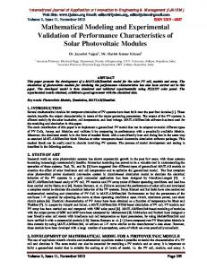
The denominator of Eq. 19 is a second order polynomial, so it represents the second order dynamics of the rotor on the axial electrodynamic bearing. In what follows, a simple numerical resolution for every rotating speed has been carried out. It should give a sufficient insight of the system behavior. Figure 4 shows the evolution of the root-loci for increasing rotation speeds.

Figure 4: Root locus related to the axial dynamic behavior of a rotor supported by axial electrodynamic bearing. Both poles are always in the left hand side of the complex plane, then the system is stable. For low rotating speed the stiffness is very small while the damping contribution is higher than the critical damping then the poles lie on the real axis. For increasing rotating speed the damping decreases while the stiffness value increases and the poles move towards the imaginary axis. For  m   they reach the imaginary axis becoming a complex conjugate pair. Axial EDB Experimental Validation A test bench for the complete levitation of a vertical axis rotor has been designed and assembled in order to validate experimentally the model of the axial electrodynamic bearing. Description of the Test Rig. In this section a test rig for the complete levitation of a rotor by means of passive bearings only is presented. In particular the radial levitation is obtained using passive reluctance bearings, while the axial levitation is achieved by means of an axial electrodynamic bearing. Fig. 5a shows a picture of the test rig. The experimental test rig, characterized by a vertical axis as shown in figures 5a and 5b, is accurately described in [22]. The main parts of the test rig are: 1) permanent magnet radial bearings, which make possible the radial levitation of the rotor; 2) electrodynamic thrust bearing, which allows to achieve the axial levitation; 3) eddy current dampers, used to introduce non rotating damping in the system; 4) ironless permanent magnet synchronous motor, to put in rotation the shaft; 5) touchdown bearings, which work at rest or at low speed before the rotor starts to levitate. Fig. 5b gives an insight about the position of the subsystems. A vertical axis configuration has been chosen because of its symmetrical geometry in comparison with a horizontal axis system. The complete magnetic levitation, in both axial and radial directions, has been achieved by means of a combination of electrodynamic axial bearing and permanent magnet radial bearings. This combination, i.e. permanent magnet axial bearing and electrodynamic radial bearings has already been studied in [14]. A radial electrodynamic bearing is in principle possible as well.

Figure 5: Axial bearing test rig. a) Test rig picture. b) Test rig subsystem’s description. The height of the rotor is 405 mm and its total weight is about 3 kg. The cross-section of the whole system (as seen from above) is square with the side lengths of 250 mm. The total height of the system is about 500 mm. Model of the Test Rig. The model of the axial bearing under quasi static operating condition described in the previous section can be adopted for the model of the test rig since the presence of the other subsystems do not affect the behavior of the overall system.. By converse, the axial dynamic behavior of the test rig is affected by the presence of the radial permanent magnet bearings and damping system. Permanent magnet bearings are composed of two permanent magnets in attractive configuration; then they introduce the desired amount of radial positive stiffness which guarantees the radial stability, but also an undesired amount of axial negative stiffness which makes the system axially unstable. This last effect is relevant for studying the axial dynamic behavior of the system, since the axial stability of the system is determined by the whole amount of axial stiffness. The damping system instead does not affect the stability of the system, but it influences its dynamic behavior as depending on the amount of axial damping introduced the vibrating response of the system at a certain rotating speed will be more or less damped.

Figure 6: Bond graph model of the dynamic behavior of the test rig.

Figure 6 represents the bond-graph model of a rotor axially supported by means of an electrodynamic bearing, radially by using passive permanent magnet bearings, and furthermore the effect of the damping system is taken into account. The states of the system are: 1) the momentum of the mass m ; 2) the flux linked by the coils  ; 3) the elongation of the spring represented by the stiffness k n . The equation of motion which rules the system is:

m  z  Fz  Fkn  FCext  Fext

(20)

where the force developed by the axial bearing Fz is described by Eq. 17 and the forces Fkn and FCext can be written as Fkn  k n  z

(21)

FCext  cext  z

The equation of motion of the rotor (Eq. 20), of the force developed by the bearing Fz (Eq. 17) and the force of the stiffness and damping (Eq. 21) can be solved together leading to the characteristic equation of the overall system 2  20   20  p e      z  Fext .  m  z   2  c  z    k ext n  L    2   L  2   2  e p e p    

(22)

The use of the Laplace's transform on Eq. 22 leads to the transfer function:

z s   Fext s 

1 s2  s 

 20    p  cext   L    e2  2p

. 

2 2 0  L e e2  2p

(23)

 kn

The poles of the system described by Eq. 23 are obtained for each value of the rotating speed. Figure 7 shows the behavior of the poles of the system. It is worth to note that the pole s1 is responsible for the instability of the system for speeds lower than the threshold  s being in the right hand side of the plot for  m   s . At  s the positive axial stiffness k generated by the bearing, is equal to the introduced negative stiffness k n , and consistently with the Earnshaw's theorem the system becomes stable.

Figure 7: Root locus related to the axial dynamic behavior of a rotor supported by axial EDB, taking into account the negative stiffness k n contribution due the presence of passive radial bearing and the axial damping c ext . The root loci plot of Fig. 7 has been obtained by considering k n  2000N / m and c ext  10 Ns / m . For  s  323rad / s the pole s1 crosses the imaginary axis towards the left side of the map and the rotor starts to levitate in a stable way. This result has been confirmed by experimental tests. The behavior of the system can be analyzed at the limit conditions:  e  0 ,  e   .

It is worth to note that for  e  0 the poles are real while for  e   they become complex conjugate pair. The vibrating response of the system is damped, according to the amount of cext introduced, even for  e   and this is the main effect of the addition of an external damping contribution. If no external damping is introduced in the system, for  e   the system will be undamped. Experimental Results. The experimental tests are addressed to the calibration of the main parameters of the model and to study the quasi static behavior of the system with the aim of validating the developed model. The quasi static behavior of the system has been accurately analyzed and experimentally validated while the dynamic performance has been evaluated in a less precise way considering solely the rotating speed threshold for the levitation. Calibration of the Model. The calibration of the model parameters is requested in order to achieve numerical results which well represent, from a quantitative point of view, the behavior of the system. Since the model of the axial bearing is based on the hypothesis that the flux distribution in axial direction   z  is linear for small axial excursions z from the nominal position z 0 , the value  0 must be experimentally evaluated. It can be found out by measuring the BEMF generated in a single coil for a fixed axial displacement z at a constant rotating speed. The value of  0 can be identified by means of a fitting between the experimental BEMF acquired and the BEMF described by Eq. 2. The best agreement between experimental and

numerical curves has been obtained for  0  5.3Wb / m . Quasi-static Analysis. The experimental validation of the model under quasi static operating conditions can be done by measuring the force and the torque produced by the bearing as function of axial displacement and rotating speed. Tests setup. For the steady state tests five requirements are needed: 1) the measure of the axial force produced by the bearing; 2) the acquisition of the rotating speed; 3) the measure of the current flowing in the coils of the axial bearing; 4) a constrain on the axial movement of the rotor; 5) the introduction of an axial displacement with respect to the nominal position. In order to measure the force developed by the bearing in axial direction the test rig has been equipped with a load cell HBM S2, characterized by: maximum force 500N, accuracy 0.05N. The load cell is located in the lower part of the rig as shown in Fig. 5 a. For what concerns the rotating speed  , since there is a synchronous motor in the rig, it can be acquired by the inverter which drives the motor. The current measure has been made by means of a current probe placed on the wire used to close the coils in a short-circuit and an oscilloscope. The axial degree of freedom is locked by acting on the adjustment of the upper touch down layer: it must be moved downward until it is in contact with the upper tip of the shaft. Considering that the contact between the rotating shaft and the load cell takes place on a screw located on the upper surface of the load cell, the introduction of the desired axial displacement of the rotor is performed by turning in clockwise or anticlockwise direction the screw. Under this operating condition (fixed axial displacement and  constant) constant forces are measured by the load cells connected to the HBM MGC plus measure amplifier system. In the test performed the axial displacement from the nominal position is included in the range 1  3 mm, while the speed range is 0  6000 rpm. The tests at steady state are carried out by measuring the force and the currents flowing in the coils for a rising of rotation speed. The rotating speed must increase up to the desired value in an appropriate time and then kept constant for a certain time. This time can't be too short in order to guarantee the steady state condition, and it can't be too long to avoid the thermal problem due to the heating of the coils. Fig. 8a describes the behavior of the axial force Fz as function of the rotating speed  m for axial displacement from the nominal position z  1.5mm . Despite the accuracy of the force measurements provided by the load cell is not constant in the whole rotating speed range because lots of vibration occur for certain speed and consequently the force measurement becomes noisy, it shows a good agreement between the analytical and the experimental results. Fig. 8 shows the comparison between the braking torque analytically computed and the one coming from the current measurement considering that all the electric power becomes mechanical power: T

i2 R . m

(24)

Fig. 8b highlights the coherence between the results experimentally and analytically obtained. The consistency between the experimental data and analytical results under quasi static operating condition is considered a proof of the validity of the developed model.

a)

b)

Figure 8: Quasi-static behavior for the axial displacement z  1.5 mm. a) Axial force Fz as function of the rotating speed  m . b) Braking torque T as function of the rotating speed  m . Conclusions A model of electrodynamic axial bearings is presented in the first part of the paper. The model, which takes the R-L dynamics into account, can be used to study both the quasi-static and the dynamic behaviors. The quasi static behavior has been analyzed by studying the axial stiffness, the force and the torque produced by the bearing working at a fixed axial position as function of the rotating speed while the dynamic behavior has been analyzed by plotting the root loci of the system according to the rotation speed. The second part of the paper is devoted to the experimental validation of the developed model. This has been done by realizing a test rig for the complete levitation of a rotating shaft only by passive means. The test rig has been equipped with a load cell to perform the quasi static test. The comparison of the analytical and experimental results, in terms of force and torque generated by the bearing, is satisfactory and can be considered as a proof of the model validity under quasi static conditions. The dynamic performance of the system have been analytically evaluated by means of a model of the test rig taking into account the negative axial stiffness introduced by the radial permanent magnet bearings and the axial damping due to the damping system. The rotating speed threshold pointed out by the model is experimentally confirmed by the behavior of the rotor of the test rig which starts the stable levitation only when the rotating speed threshold is overcome. REFERENCES 1. Post, R. F., and Ryutov, D. D., 2000, The Inductrack: A Simpler Approach to Magnetic Levitation, IEEE Trans. Appl. Supercond., 10, pp. 901--904. 2. Thornton, R. D., and Thompson, M. T., 1997, Magnetically Based Ride Quality Control for an Electrodynamic Maglev Suspension, Proceedings of the Fourth International Symposium on Magnetic Suspension Technology, Gifu City, Japan, Oct. 30--Nov. 1, pp. 303--311. 3. Basore, P. A., 1980, Passive Stabilization on Flywheel Magnetic Bearings, MS thesis, Massachusetts Institute of Technology, Cambridge, MA. 4. Post, R. F., and Ryutov, D. D., 1998, Ambient-Temperature Passive Magnetic Bearings: Theory and Design Equations, Proceedings of the Sixth International Symposium on Magnetic Bearings, Massachusetts Institute of Technology, Cambridge, MA, Aug. 5--7, pp. 109--122.

5. Bender, D. A., and Post, R. F., 2000, Ambient-Temperature Passive Magnetic Bearings for Flywheel Energy Storage Systems, Proceedings of the Seventh International Symposium on Magnetic Bearings, ETH Zurich, Switzerland, Aug. 23--25, pp. 153--158. 6. Lembke, T. A., 2003, Induction Bearings, a Homopolar Concept for High Speed Machines, Ph.D. thesis, Royal Institute of Technology, Stockholm, Sweden. 7. Lembke, T. A., 2004, 3D-FEM Analysis of a Low Loss Homopolar Induction Bearing, Proceedings of the Ninth International Symposium on Magnetic Bearings, Lexington, KY, Aug. 3--6. 8. Girardello Detoni, J., 2008, "Modellistica di cuscinetti elettrodinamici", Thesis, Politecnico di Torino, Turin, Italy. 9. Murakami, C., and Satoh, I., 2000, Experiments of a Very Simple Radial-Passive Magnetic Bearing Based on Eddy Currents, Proceedings of the Seventh International Symposium on Magnetic Bearings, ETH Zurich, Switzerland, Aug. 23--25, pp. 141--146. 10. Filatov, A., and Maslen, E. H., 2001, Passive Magnetic Bearing for Flywheel Energy Storage Systems, IEEE Trans. Magn., 37, pp. 3913--3924. 11. Filatov, A., 2002, Null-E magnetic bearings, PhD thesis, University of Virginia, Charlottesville, USA. 12. Filatov, A., 2006, Flywheel energy storage system with homopolar electrodynamic magnetic bearing, Proceedings of the tenth international symposium on magnetic bearings, Martigny, Switzerland. 13. Moser, R., Regamey, Y.-J., Sandtner, J., and Bleuler, H., 2002, Passive Diamagnetic Levitation for Flywheels, Proceedings of the Eighth International Symposium of Magnetic Bearings, Mito, Japan, Aug. 26--28, pp. 599--603. 14. Sandtner, J., and Bleuler, H., 2004, Electrodynamic Passive Magnetic Bearing With Planar Halbach Arrays, Proceedings of the Ninth International Symposium on Magnetic Bearings, Lexington, KY, Aug. 3--6. 15. Sandtner, J., and Bleuler, H., 2006, Passive Electrodynamic Magnetic Thrust Bearing Especially Designed for Constant Speed Applications, Proceedings of the Tenth International Symposium on Magnetic Bearings, Martigny, Switzerland, Aug. 21--23. 16. Tonoli, A., 2007, Dynamic Characteristics of Eddy Current Dampers and Couplers, J. Sound Vib., 301, pp. 576--591. 17. Genta, G., Macchi, P., Carabelli, S., Tonoli, A., Silvagni, M., Amati, N., and Visconti, M., 2006, Semi-Active Electromagnetic Dampers for the Dynamic Control of Rotors, Proceedings of the Seventh IFToMM---Conference on Rotordynamics, Vienna, Austria, Aug. 23--25, pp. 1--10. 18. Tonoli, A., and Amati, N., 2008, Dynamic Modeling and Experimental Validation of Eddy Current Dampers and Couplers, ASME J. Vibr. Acoust., 130, pp. 021011-021011. 19. Amati, N., De Lépine, X., Tonoli, A., 2008, "Modeling of Electrodynamic Bearing", ASME J. Vibr. Acoust., 130, pp. 061007-1- 061007-9. 20. Genta, G., Dynamics of Rotating Systems, 2004. 21. S.H. Crandall, D.C. Karnopp, E.F. Kurtz, E.C. Pridmore-Brown, Dynamics of Mechanical and Electromechanical Systems, McGraw-Hill, New York, 1968. 22. Impinna, F., Electrodynamic bearings Modeling and Design, PhD thesis, Politecnico di Torino (Italy), 2010.