electro-mechanic antagonistic actuation to asymmetric im- plementations in which ... inertia to the drive train between the positioning motor and the link. The link ...
2010 IEEE International Conference on Robotics and Automation Anchorage Convention District May 3-8, 2010, Anchorage, Alaska, USA
Dynamic Modelling and Control of Variable Stiffness Actuators Alin Albu-Sch¨affer, S. Wolf, O. Eiberger, S. Haddadin, F. Petit, and M. Chalon German Aerospace Center (DLR) Oberpfaffenhofen, D-82234 Weßling, Germany, http://www.dlr.de/rm/
Abstract— After briefly summarizing the mechanical design of the two joint prototypes for the new DLR variable compliance arm, the paper exemplifies the dynamic modelling of one of the prototypes and proposes a generic variable stiffness joint model for nonlinear control design. Based on this model, the design of a simple, gain scheduled state feedback controller for active vibration damping of the mechanically very weakly damped joint is presented. Moreover, the computation of the motor reference values out of the desired stiffness and position is addressed. Finally, simulation and experimental results validate the proposed methods.
I. I NTRODUCTION Variable Impedance Actuation (VIA) is considered by many researchers as the next big design step towards robots with increased mechanical robustness during impacts or in contact with unknown environments. Furthermore, approaching the performance of humans in terms of force and speed at same arm weight is expected with this new technology. Therefore, VIA actuation is a very active topic of ongoing research [1], [2], [3], [4], [5], [6], [7], [8], [9]. Currently, a hand-arm system with variable compliance is designed at DLR, incorporating in a first, concept validation version, several variable compliance joint designs for fingers and arms. For the elbow and the shoulder, the focus is on energy efficient and weight minimizing design, such that the mass of the VIA joints do not considerably exceed the weight of the DLR LWRIII [10] joints. Although inspired by the human muscle actuation, most of today VIA mechanisms differ from the human archetype by having a very low, intrinsic damping. They are thus better described by the term ”variable stiffness mechanism” (VSA). The high compliance and low damping make the control challenging. Regarding the control of VSA, literature mostly deals with the problem of adjusting stiffness and position of the actuator in a decoupled manner, by controlling the position or the torque of the two motors of the joint [4], [5], [2]. Moreover, in case of VSA structures with many degrees of freedom (dof) and cable actuation, the decoupling of the tendon control is a challenging issue, treated for example in [11], [12]. Our approach to the control of the VSA arms starts from the passivity based control framework developed for the torque controlled light-weight robots [13] and is based on a state feedback controller with variable gains. Some particular aspects compared to the control of flexible joint robots with fixed compliance [13], [14], [15] are summarized below: • Due to the high compliance of the joint, a separate torque sensor is not required any more, the torque can
978-1-4244-5040-4/10/$26.00 ©2010 IEEE
be well estimated based on the motor and link position and compliance properties [16]. • An active compliance control will be used only for stiffness components which cannot be realized by the mechanical springs. Examples are zero stiffness or the joint coupling stiffness1 needed to achieve arbitrary Cartesian stiffness matrices [17]. It is desired that the mechanical joint compliance corresponds as close as possible to the desired task compliance. • The joints have very low intrinsic damping. While this is useful for cyclic movements involving energy storage (e.g. for running or throwing), the damping of the arm for fast and precise positioning tasks has to be realized by control. This is a challenging task in view of the strong variation of inertia and stiffness. It turns out that due to the very low stiffness, the passivity framework has to be given up for high performance vibration damping, which in this case requires an aggressive, strongly model based strategy. The above mentioned control aspect will be detailed in Section IV after briefly summarizing the mechanical design of the joints in Section II and presenting modelling aspects in Section III. Finally, Section V provides simulation and experimental results. II. H ARDWARE D ESIGN C ONCEPTS FOR THE DLR ARM JOINTS
There are currently many design approaches for realizing variable compliance actuators, ranging from pneumatic or electro-mechanic antagonistic actuation to asymmetric implementations in which one positioning motor is used to move the joint and a second, smaller actuator is used to adjust the stiffness. In our approach, which follows the latter concept, the positioning motor is connected to the link via a harmonic drive gear. Mechanical compliance is introduced by a mechanism which forms a flexible rotational support between the harmonic drive gear and the joint base (Fig. 1). In case of a compliant deflection of the joint, the whole harmonic drive gear rotates relatively to the base, but the positioning motor is not moved. So the link side inertia is altered only by the circular spline and some parts of the variable stiffness device. The spring mechanism adds no inertia to the drive train between the positioning motor and the link. The link position is changed without moving the elasticity mechanism.
2155
1 realizes
in biological systems by biarticular muscles
flex spline (qf ) Harmonic Drive gear
spindle
wave generator (qw )
spring base slider
stiffer preset
connection to linear bearing
translational deflection
circular spline (qc )
roller slider cam rollers
variable stiffness mechanism
cam disk
Fig. 1. Principle of variable stiffness joint mechanics in differential gear setup. The circular spline of the harmonic drive gear is supported by the mechanism.
joint deflection
axis of rotation
(fixed to circular spline)
Fig. 3. VS-Joint mechanism. The joint axis is in the vertical direction. The cam disk rotates due to the compliant joint deflection. This results in a vertical displacement of the roller slider. A stiffer joint preset is achieved by moving the spring base downwards. stiffness actuator
J linear bearing roller
roller position of undeflected link
J
r deflection
Fig. 4. Unwinded schematic of the VS-Joint principle in centered (a) and deflected (b) position. A deflection of the link results in a horizontal movement of the cam disk and a vertical displacement of the roller. The spring force generates a centering torque on the cam disk.
section will focus on this joint, while the controller structure and the experimental results are given for both the VS and the QA joint, which will be presented next. Fig. 2. Variable impedance joint prototype. Two different implementations of the compliance element have been integrated and tested.
Two different mechanical compliant joint concepts have been derived from the previous considerations at DLR. Fig. 2 shows a joint testbed which can incorporate both compliant joint principles and on which the experiments have been conducted. A short overview of the principles is given next. A. Variable Stiffness Joint Design The concept of the Variable Stiffness Joint (VS-Joint) as presented in [16] contains two motors of different size. The high power motor changes the link position. The joint stiffness is adjusted by a much smaller and lighter motor, that changes the characteristic of the supporting mechanism (Fig. 3). An unwinded schematic of the principle is shown in Fig. 4. A compliant link deflection results in a displacement of the cam disk and is counterbalanced by the roller pressed on it in axial direction by a spring. This generates a centering force resulting in the output torque of the link. To change the stiffness preset, the smaller motor moves the spring base axially w.r.t. to the cam disk and thus varies the spring force. The joint prototype can be equipped with different cam disks. This permits an easy adaption of the passive joint behavior to the desired application by designing the torque/deflection characteristic of the joint. The modelling
B. Quasi Antagonistic (QA) Joint Mechanism Like the VS-Joint, the QA joint consists of a link positioning motor with harmonic drive gear and the elastic mechanism with the stiffness actuation motor [18]. Two cam-roller systems, each supplied with a spring, operate in an opposing setup. The main difference compared to a classical antagonistic joint is that the two motors are not used in a symmetrical configuration as agonist and antagonist. Instead, one motor adjusts the link side position, while the second motor produces a co-contraction of the two cam-roller systems and thus operates stiffness adjustment (Fig. 5). This arrangement reduces dynamic losses and allows stiffness adjustment independent from the link speed by a stiffness actuator that is optimized for this purpose. This special form of antagonistic actuation is very advantageous for configurations with pronounced agonist actuation, in which the adjusting motor does not have to produce a holding torque. The cam-roller mechanism generates a nonlinear spring characteristics. The shape of the cam faces can be adapted to provide any desired progressive torque characteristic that stores the same maximum potential energy in the linear spring. Superposition of agonist and antagonist with different offsets results in the desired variable stiffness. Fig. 7 shows the realization of the QA joint compliance mechanism.
2156
motor 1
The position r of the roller in the variable spring mechanism (Fig. 4) is related to qc by the nonlinear function f1 representing the geometry of the cam-disk: r = f1 (qc ) := f (q − θ). Furthermore, we denote by σ the position of the stiffness adjusting motor. Using these variables, the potential energy P and the kinetic energy T of the system can be expressed as:
motor 1
motor 2
(a)
motor 2
(b)
Fig. 5. Variable Stiffness Actuator with nonlinear progressive springs in antagonistic (a) and quasi antagonistic (b) realization. In the latter case, Motor 1 moves the joint while Motor 2 is adjusting the stiffness. cam bar
connection to circular cpline
rocker arm
spring stiffness actuator Fig. 6.
Cross section of the Quasi Antagonistic Joint design.
III. M ODELLING OF THE VSA J OINTS The modelling of the VS-Joint is given as an example before proposing a generic model structure. The kinematics of the harmonic drive gear with reduction ratio n is given by: q˙c = αq˙f + β q˙w , (1) with q˙c , q˙f , and q˙w being the velocities of the circular spline, the flex spline, and the wave-generator, respectively (Fig. 1), and with α = n/(n + 1) and β = 1/(n + 1). For a representation independent of the reduction ratio, we introduce θ = −1/nqw , i.e. θ represents the motor angle transformed to the circular spline side of the gearbox, as usual in the modelling of flexible joint robots2. We denote furthermore the link angle by q and, since the link is attached to the flexible spline, we have q = qf . With this new notations, (1) becomes ˙ q˙c = α(q˙ − θ).
(2)
2 The minus sign comes from the fact that the wave generator and the flex spline rotate in opposite directions.
Fig. 7.
2P = k(σ − r)2 = k(σ − f (q − θ))2 , ˙ 2 + Jθ θ˙2 + Jq 2 + Jr r˙ 2 + Jσ σ˙ 2 . 2T = α Jc (q˙ − θ) 2
(3)
The inertia values are denoted therein by Ji with the subscript representing the related state variable, i.e. i ∈ (q, qc , θ, σ, r). In these equations, only the positions q, θ, and σ and their derivatives are independent state variables. By applying the Lagrangian formalism to (3) one obtains (4), see next page. (q−θ) 2 The notations jr = df d(q−θ) and Jrv = jr Jr are used in (4). Please note that Jrv is a state dependent, thus variable inertia term caused by the nonlinear transformation of the roller inertia from roller coordinate to the circular spline coordinate. Accordingly, centrifugal terms, denoted by cθ and cq are associated to the variation of this inertial term. The control inputs are the torques of the joint actuator and of the stiffness actuator τθ and τσ , respectively, while τext is the external torque acting on the joint. Comparing this model with that of the QA joint (not presented here for brevity) and of other VSA joint prototypes [19], we think that a reasonably general abstraction of a variable stiffness actuator which can be used for the generic design of controllers for VSA devices is given by ∂V (x) τ1 τ2 ˙ + M (x)¨ x + c(x, x) = , (5) ∂x τ ext
with the configuration vector x given by the two motor positions and the link position, with M ∈ ℜ3x3 being a variable inertia matrix, c the Coriolis and centrifugal vector, V the potential energy of the elastic element and related to the gravity forces, τ1 and τ2 the torques of the two motors. The most relevant property of this structure is its underactuation, meaning that the system has less control inputs (2) than its configuration dimension (3). However, in contrast to other underactuated systems, in this case V is positive definite, implying that an unique equilibrium point exists for each external torque and that the linearization of the system around an equilibrium point is controllable. The system belongs to the class of underactuated EulerLagrange systems, for which an impedance controller has been developed in [20], based only on measurement of motor positions and ensuring the achievement of the desired link position and stiffness. However, one topic only marginally addressed in that work was the appropriate damping of the transient behaviour. This aspect will be treated in the next section, for a simplified, linearized model. If the inertia of the roller, the circular spline, and the stiffness adjuster are much lower than the motor and link inertia3 , the nonlinear terms in (4) can be ignored and the system
Prototype of the QA variable compliance element.
3 In
2157
the case of the VS-Joint they are by two orders of magnitude lower.
Jθ + α2 Jc + Jrv −α2 Jc − Jrv 0
.
0 cθ (θ − q, θ˙ − q) ˙ −jr τθ θ¨ 0 q¨ + cq (θ − q, θ˙ − q) ˙ +k(σ−f (θ−q)) jr = τext (4) 1 τσ Jσ σ ¨ 0
−α2 Jc − Jrv Jq + α2 Jc + Jrv 0
configuration is described by θ and q only. In this case, the equation of the system reduces to � � � � �� � � τ τθ Jθ 0 θ¨ + = , (6) −τ τext + g(q) 0 Jq q¨ with τ = k(f (θ − q) − σ)jr
(7)
and with g(q) representing the gravity torques. Here, the position of the stiffness adjusting actuator σ is regarded as an input. IV. C ONTROL OF THE VS-J OINT Several paradigms of how the compliance of VSA joints has to be controlled are encountered in the literature. Our approach, similar to the one in [2], [21] is to define the desired stiffness along the desired (nominal) trajectory and to compute the preset value σ of the stiffness actuator based on these nominal values as well as on the torque of the rigid body motion along the trajectory. If the joint is perturbed by an external torque, the system should react with the intrinsic passive characteristic of the spring, meaning for example that increasing the torque increases also the stiffness. This is a desired behaviour and should not be altered by the controller by trying to regulate stiffness to a constant value in the disturbed case. Therefore, the stiffness actuator should not react in a first phase during an impact and its size can be rather small. At a slower time scale appropriate collision reaction strategies, including stiffness adjustment, can be designed [22]. The very weakly damped system, however, needs to be damped by the controller through the joint motor4 . Moreover, in order to provide a precise link side motion, the high compliance has to be taken into account when computing the desired motor angles. A first, pragmatic approach to the control of the joint was a gain scheduling controller for the linearized dynamics along the nominal trajectory. In absence of external torques, the linearized dynamics is
a passivity based stability and convergence analysis for the original nonlinear model, as described in [13]. The ˙ ∆q, ∆q) states for the system are (∆θ, ∆θ, ˙ or, alternatively, ˙ (∆θ, ∆θ, ∆τ, ∆τ˙ ). However, due to the strong variation of kφ and of the link inertia when the actuator is used in a multidof robot, the vibration damping performance of a constant gain controller is very poor for stiffness values for which it was not optimized. Consequently, for the VSA joints, the controller gains (and thus the eigenvalues for the linearized system) are scheduled depending on the stiffness kφ and the link inertia Jq . The controller is ˙ τθ = τθ f f + kp θ˜ + kd θ˜ + kt τ˜ + ks τ˜˙ ,
(12)
Jθ , Jq , kφ , ∂g(q) ∂q .
with the gains kp , kd , kt , ks depending on ˙ ˙ The error variables are θ˜ = ∆θd − ∆θ, θ˜ = ∆θ˙d − ∆θ, ˙ τ˜ = ∆τd − ∆τ , τ˜ = ∆τ˙d − ∆τ˙ . The desired torque for the controller is τd = Jq q¨d + g(qd ). (13) The gains are optimized in each controller step in order to: • Provide the desired critical damping factors ξ for the linearized system X (ξj − 0.707)2. (14) argmin kp ,kd ,kt ,ks
j
In principle, a linear feedback controller with constant gains can be designed for the linearized system, which enables
Keep the control gains within practically feasible value ki min ≤ ki ≤ ki max with i ∈ (p, d, s, t). The gains have to be high enough to overcome friction and low enough not to excite un-modelled dynamics and to avoid actuator saturation. Remark 1 The passivity based analysis from [13] does unfortunately not apply to this controller mainly for two reasons: a) It was not possible to find controller gains with fixed kp over the whole range, which to perform satisfactory. Constant (or integrable) kp was a condition for easily finding a Lyapunov function in [13]. b) For damping the very compliant, weakly damped joint5 , a high ks gain is required, which in some cases does not fulfill the passivity condition regarding damping from [15]. Therefore, for stability analysis, one has to rely so far on the local statement of Lyapunov’s indirect method. Remark 2 Optimizing the control gains is generally difficult, because the large variation of the instantaneous stiffness often requires gains which exceed the mentioned bounds. We expect that similar problems would arise in practice with more advanced, nonlinear controllers, such as nonlinear passivity based approaches, back-stepping or feedback linearization: One has to very carefully design the target dynamics for obtaining practically feasible gains. One possible approach would be to use the eigenvalues of the simple
4 Note that the stiffness adjusting motor can have only minor contribution to vibration damping due to its low power.
5 For sake of simplicity, the (very low) intrinsic damping of the joint was completely omitted in the modelling part.
Jθ ∆θ¨ + kφ ∆φ ∂g(q) ∆q Jq ∆¨ q − kφ ∆φ + ∂q
= ∆τθ
(8)
= τext ,
(9)
with φ = θ − q and the instantaneous stiffness computed as "� # �2 ∂f (φ) ∂ 2 f (φ) kφ = k (10) + (f (φ) − σ) ∂φ ∂φ2 The feed-forward motor torque on the nominal trajectory is τθ f f = Jθ θ¨d + Jq q¨d + g(qd ).
(11)
•
2158
linearization based controller as linear target dynamics and design nonlinear controllers to exactly fulfil it. This is a topic for further work. A. Setting the Desired Compliance and Link Angle While the previous section is concerned with the problem of damping the joint oscillations for situations in which a smooth, vibration-free motion is the control objective, there are two further relevant aspects for the control of the joint: • The achievement of the desired link position in nominal conditions (no external interaction), with the control based only on motor position and torque feedback. It is required to have a good positioning performance while preserving the mechanical compliance properties of the joint as much as possible - the total compliance would be altered if the controller would use link position feedback.
Kd
σd
τd Fig. 8. Torque/stiffness diagram for the VS-Joint, parameterized over the stiffness preset σ. This diagram can be used for determining stiffness preset which has to be commanded for reaching a specified desired stiffness, given a nominal joint torque. VS-Joint Torque 250
200
Ensuring a specified joint compliance ktot along the nominal trajectory. This compliance is specified by the application. Note that due to the feedback of the motor position θ and of the torque τ , the total stiffness is composed of the controller stiffness kp (P-term) in serial interconnection with the mechanical instantaneous stiffness kφ and reduced by the torque feedback. ktot =
kP kφ kP + (kt + 1)kφ
(15)
This results from (8),(9),(12) at steady state. Given the current torque and the specified ktot one has to chose kφ in the feasible range (see Fig. 11) and compute afterwards kp as kp =
kφ ktot (kt + 1) . kφ − ktot
(16)
Obviously, kp has to go down to zero if the desired stiffness ktot approaches zero. The gravity compensation, however, cannot be done based on desired position in this situation, but online gravity compensation as in [13] has to be used. For solving both position and stiffness preset, one can start from the nominal torque of the rigid body dynamics along the nominal trajectory τd = Jθ q¨d + g(qd ).
(17)
Torque (Nm)
•
σ σ σ σ
= = = =
0 1/3 ∗ σmax 2/3 ∗ σmax σmax
150
100
50
0 0
2
4
6
8
10
12
14
Deflection (deg)
Fig. 9. Deflection/torque diagram for the VIA joint, parameterized over the stiffness preset σ. This diagram can be used for determining the motor position which has to be commanded for reaching a specified link position.
in order to reach the desired link position despite of the compliance of the joint and of the controller. The controller structure is visualized in Fig. 10. V. S IMULATIONS AND E XPERIMENTAL R ESULTS First, some simulations with the QA and the VS-Joint are given to illustrate the topics addressed in the previous section. Thereafter, experimental results are presented. A. Simulations Fig. 12, left column, shows the the behaviour of the VSJoint for a high stiffness (100% preset). On the plots, the settling of the system for non-zero initial conditions as well as a step position response are simulated. On the position plot (a) one notices that the motor has to follow an oscillating
For a given τd and a specified kφ , it is possible to compute analytically the preset value σd for the stiffness actuators of the DLR joints. The solution is visualized graphically in Fig. 8 for the VS-Joint. In Appendix A, an analytical solution is given for the QA joint. This solves the problem of stiffness preset. Using the preset σd and the torque τd , it is further possible to compute analytically the deflection of the compliant element φd . The dependency for the VS-Joint is visualized in Fig 9, while, again, the analytical result for the QA joint is given in the Appendix. It is then straight forward to compute the desired motor position as τd (18) θd = qd + φd + (kt + 1) kp
2159
Jq
DLR VIA Joint
J T
J T
k G
d
J V
, ,k �
W
W
G
Fig. 10.
Controller structure of the DLR variable impedance joints.
(a) − positions
(a) − positions
0.95
0.9 0.88
0.9
feasible mechanical stiffness range 0.86
angles [rad]
0.85
angles [rad]
0.84 0.82 0.8
q
qd
d
0.78
0.7
q
0.76
θ θ
0.74 0.72
0.8
0.75
q θ θ
0.65
d
0
0.2
0.4
0.6
0.8
1
1.2
1.4
1.6
1.8
d
2
0
0.2
0.4
0.6
1.5
2
1.5
0.8
1
1.2
1.4
1.6
1.8
2
time [s] (b) − velocities
time [s] (b) − velocities
1
Fig. 11. Torque/stiffness diagram for the QA joint. The available mechanical stiffness range is exemplified for a torque τd , e.g. corresponding to the gravity load of the robot in a given configuration.
velocity [rad/s]
d
velocity [rad/s]
1 W
0.5
0
0.5
0
−0.5
−0.5
dθ
−1
dθ
−1
dq
dq −1.5
0
0.2
0.4
0.6
0.8
1
1.2
1.4
1.6
1.8
−1.5
2
0
0.2
0.4
0.6
time [s] (c) − torque
B. Experimental results The model has been validated by measurements on the joint test-bed. Special care has been taken to confirm the stiffness characteristics of the joint and to identify the friction of the compliance mechanism. This friction, in contrast to the gearbox friction, is very critical, since it leads to a dead zone in the torque measurement and also to an uncertainty in the positioning of the link for a given motor position. For the VS-Joint, this friction turned out to be very low, see Fig. 15. Friction measurements for the QA joint can be seen in [18]. Therefore, it was easy to transfer the controller developed in simulation to the real joint. Two main positive implementation aspects came out: • due to the high compliance and low friction, the torque estimation based on the joint deflexion φ = θ − q is very accurate. Therefore it seems that it is possible to eliminate the torque sensor without loss of performance.
1
1.2
1.4
1.6
1.8
2
1.4
1.6
1.8
2
1.4
1.6
1.8
2
time [s] (c) − torque
10
10
0 0
joint torque [Nm]
joint torque [Nm]
−10 −10
−20
−30
−20
−30
−40
−50 −40 −60
−50
0
0.2
0.4
0.6
0.8
1
1.2
1.4
1.6
1.8
2
−70
time [s] (e) − stiffness
0
0.2
0.4
0.6
0.8
1
time [s]
1.2
(e) − stiffness
650
1200
600 1000
joint stiffness [Nm/rad]
550
joint stiffness [Nm/rad]
motion during the transients in order to provide a smooth link side motion. The strong effect of the elasticity can be seen also on the velocity plots Fig. 12(b), by noticing the strong difference between motor and link velocity. Fig. 12(c) shows the spring torque, while Fig. 12(d) shows its spatial derivative, the stiffness. One can see that the stiffness varies by more than a factor of two during motion. The same plots are shown for a stiffness preset corresponding to a low stiffness (10% preset) in the right column of Fig. 12. One can observe that in both situations the motion is properly damped, thus the main control objective has been reached. The controller remains always stable, despite of the strong nonlinearity in the stiffness. One can also notice that for the low stiffness, the settling time is slower. In Fig. 13 the simulation is repeated with the QA joint. Also for this system, which has a very different stiffness characteristics from the VS-Joint (compare Fig. 11 and Fig. 8), the vibration damping has the desired performance. As a comparison, Fig. 14 shows the behaviour of the system when using only a PD controller on motor side, without vibration damping. While the motor position is relatively well controlled, the link side displays very strong oscillations due the the very low damping of the spring.
0.8
500 450 400 350 300
800
600
400
250 200
200 150
0
0.2
0.4
0.6
0.8
1
time [s]
1.2
1.4
1.6
1.8
2
0
0
0.2
0.4
0.6
0.8
1
1.2
time [s]
Fig. 12. Simulation results for 1 dof VS-Joint with high stiffness preset (left) and low stiffness preset (right).
The feedback gain for the time derivative of torque, which for rigid robots is sometimes critical, can be chosen relatively high. This enables an effective vibration damping. However, this also implies a non-passive controller. Fig. 16 shows the performance of the positioning experiments for a very low as well as for a very high stiffness preset of the VS-Joint. The experiments confirm the results and the control performance predicted by the simulation. Finally, Fig. 17 compares the reaction of the QA joint to a hard impact to the link with PD-control (upper) and state feedback control (lower). The faster dissipation of the impact energy in the latter case can be clearly observed. •
VI. C ONCLUSION The paper addressed the modelling and control of two DLR variable stiffness joint prototypes. We proposed a quite general model structure which covers in our opinion a wide range of VIA joint designs. Moreover, we addressed the stiffness and position setting and the vibration damping
2160
0.86
0.86
2
0.84
0.84
0.84
0.8
q
0.8
q
d
0.4
0.6
0.8
1
1.2
1.4
1.6
1.8
2
dθ
0.6
0.8
1
1.2
1.4
1.6
1.8
2
0
dq
1 0.5 0
1.5 1 0.5 0
−0.04 −0.06
1.8
2
20
20
10
10
joint torque [Nm]
30
0
−20 −30
0.6
0.8
1
1.2
1.4
1.6
1.8
−60
2
0
800
800
joint stiffness [Nm/rad]
900
300 200
0.8
1
1.2
1.4
1.6
1.8
2
1.4
1.6
1.8
2
time [s] (e) − stiffness
0.8
1
1.2
1.4
1.6
1.8
2
700 600 500 400 300 200
0
0.2
0.4
0.6
0.8
1
1.2
1.4
1.6
1.8
2
100 0
time [s]
0.2
0.4
0.6
0.8
1
1.2
time [s]
100
1000
400
0.6
Evaluation of Torque Estimation
900
500
0.4
150
1000
600
0.2
Fig. 14. Simulation results for 1 dof QA joint with high stiffness preset and no vibration damping. One can observe the strong oscillations due to the very low intrinsic damping of the joint.
0.2
0.4
0.6
time [s] (e) − stiffness
700
0
−30
−50
0.4
0.6
−20
−40
0.2
0.4
0
−50
0
−1.5
−10
−40
−60
0.2
time [s] (c) − torque
30
−10
−0.12
0
0.8
1
1.2
1.4
1.6
1.8
Torque Calculated (Nm)
1.6
−1
2
−0.02
−1.5 1.4
1.8
800
−1.5
1.2
1.6
0
−0.1
1
1.4
900
−1
time [s] (c) − torque
1.2
0.02
−1
0.8
1
1000
−0.08
0.6
0.8
0.04
−0.5
0.4
0.6
0.06
−0.5
0.2
0.4
dq
2
1.5
0
0.2
1 0.5
time [s] (d) − deflection
dθ
2.5
velocity [rad/s]
velocity [rad/s]
0.4
3
3
2
0.2
dq
1.5
−0.5
θ θd
time [s] (b) − velocities
time [s] (b) − velocities 2.5
0
0.72
dθ
0
q
joint stiffness [Nm/rad]
0.2
qd
0.74
d
joint deflection [rad]
0
0.72
0.8
0.76
θ θ
0.74
d
0.82
0.78
q
0.76
θ θ
0.74
d
0.78
q
0.76
0.72
0.82
velocity [rad/s]
2.5
0.86
angles [rad]
3
0.82
joint stiffness [Nm/rad]
(b) − velocities
0.9 0.88
0.78
joint torque [Nm]
(a) − positions
(a) − positions
0.9 0.88
angles [rad]
angles [rad]
(a) − positions 0.9 0.88
2
time [s] (e) − stiffness
50
0
−50
700
−100 600
σ=0 σ = σmax
500
−150 −150
400
−100
−50
0
50
100
150
Torque Sensor (Nm)
300 200
100
Fig. 15.
100 0
0.2
0.4
0.6
0.8
1
1.2
1.4
1.6
1.8
2
0
0.2
0.4
0.6
0.8
time [s]
1
1.2
1.4
1.6
1.8
Evaluation of the model of the mechanical compliance.
2
time [s]
Fig. 13. Simulation results for 1 dof QA joint with high stiffness preset (left) and low stiffness preset (right).
control design. Due to generally weakly damped springs and the high variation of instantaneous stiffness and inertia, designing a practically feasible vibration damping can be quite challenging, requiring non-passive controllers. Adding variable mechanical damping can be an alternative solution, at the cost of additional hardware complexity. However, using a good dynamic model, control based vibration damping proved to be experimentally feasible. Future work will address the design of controllers for which also global convergence conclusions can be drawn.
VII. ACKNOWLEDGEMENT
A PPENDIX For the QA joint, the joint torque and the instantaneous stiffness are described by τ kφ
= =
ae−bσ (ebφ − e−bφ ) abe−bσ (ebφ + e−bφ ),
(19) (20) (21)
where a and b are positive constants [18]. Given a current torque and a desired stiffness, one can solve the system of equations for φ and σ: � � kδ 1 −1 (22) tanh φ = b bτ τ 1 . (23) σ = − ln bφ b a (e − e−bφ ) (24) R EFERENCES
This work has been partially funded by the European Commission’s Sixth Framework Programme as part of the project PHRIENDS under grant no. 045359 and VIACTORS under grant no. 231554.
2161
[1] T. Morita, H. Iwata, and S. Sugano, “Development of human symbiotic robot: Wendy.” IEEE Int. Conf. of Robotics and Automation, pp. 3183– 3188, 1999. [2] A. Bicchi and G. Tonietti, “Fast and Soft Arm Tactics: Dealing with the Safety-Performance Trade-Off in Robot Arms Design and Control,” IEEE Robotics and Automation Mag., vol. 11, pp. 22–33, 2004.
10% of max. stiffness 100% of max. stiffness
1.2
link velocity [rad/s]
1
0.8
0.6
0.4
0.2
0
−0.2
0
0.1
0.2
0.3
0.4
0.5
0.6
0.7
0.8
0.9
1
time [s] 2
10% of max. stiffness 100% of max. stiffness
0
joint torque [Nm]
−2 −4 −6 −8 −10 −12 −14 −16 −18
0
0.1
0.2
0.3
0.4
0.5
0.6
0.7
0.8
0.9
1
time [s]
Fig. 16. Motion of the VS -Joint on a trajectory with rectangular velocity profile for small and maximal stiffness. A critically damped velocity step response can be achieved independent from the stiffness and inertia value (upper). The effect of vibration damping is clearly observed in the torque signal (lower).
J o
i n t
t o
rq u e
L
15
i n k
s p
e
e
d
2 s ] d /
5
[ ra
0 −5 −10
q _
�
[ Nm ]
10 1
0
−1
−15 −20
−2 0.5
1
1.5 t
J o
i n t
2
2.5
3
3.5
0.5
1
[ s ]
t o
t
2
2.5
3
3.5
[ s ]
rq u e
L
2
0
1.5
d /
s ]
5
[ r a
−5 −10
q _
�
[ Nm ]
1.5
−15 −20
i n k
s p
e
e
d
1 0.5 0 −0.5 −1
0.5
1
1.5 t
2 [ s ]
2.5
3
3.5
0.5
1
1.5 t
2
2.5
3
3.5
[ s ]
Fig. 17. Reaction of the QA joint on a hard link impact: with PD control (upper) and with state feedback control (lower).
[3] S. A. Migliore, E. A. Brown, and S. P. DeWeerth, “Biologically Inspired Joint Stiffness Control,” in IEEE Int. Conf. on Robotics and Automation (ICRA2005), Barcelona, Spain, 2005. [4] G. Palli, C. Melchiorri, T. Wimboeck, M. Grebenstein, and G. Hirzinger, “Feedback linearization and simultaneous stiffnessposition control of robots with antagonistic actuated joints,” in IEEE Int. Conf. on Robotics and Automation (ICRA2007), Rome, Italy, 2007, pp. 2928–2933. [5] B. Vanderborght, B. Verrelst, R. V. Ham, M. V. Damme, D. Lefeber, B. M. Y. Duran, and P. Beyl, “Exploiting natural dynamics to reduce energy consumption by controlling the compliance of soft actuators,” Int. J. Robotics Research, vol. 25, no. 4, pp. 343–358, 2006. [6] K. Koganezawa, “Mechanical stiffness control for antagonistically driven joints,” in Proc. of the IEEE/RSJ International Conference on Intelligent Robots and Systems. IEEE/RSJ, August 2005, pp. 2512– 2519. [7] C. English and D. Russell, “Implementation of variable joint stiffness through antagonistic actuation using rolamite springs,” Mechanism and Machine Theory, vol. 34, no. 1, pp. 27–40, 1999. [8] T. Morita and S. Sugano, “Development and evaluation of seven-d.o.f. mia arm,” in Proc. 1997 IEEE International Conference on Robotics and Automation, September 1997, pp. 462–467. [9] J. W. Hurst and A. A. Rizzi, “Series compliance for robot actuation: Application on the electric cable differential leg,” IEEE Robotics & Automation Magazine, vol. 15, no. 3, p. 2008, 2008. [10] A. Albu-Sch¨affer, S. Haddadin, Ch. Ott, A. Stemmer, T. Wimb¨ock, , and G. Hirzinger, “The DLR lightweight robot - design and control concepts for robots in human environments,” Industrial Robot: An International Journal, vol. 134, no. 5, pp. 376–385, 2007. [11] H. Kobayashi and R. Ozawa, “Adaptive neural network control of tendon-driven mechanisms with elastic tendons,” Automatica, vol. 39, pp. 1509–1519, 2003. [12] K. Tahara, Z.-W. Luo, R. Ozawa, J.-H. Bae, and S. Arimoto, “Biomimetic study on pinching motions of a dual-finger model with synergistic actuation of antagonist muscles,” in IEEE Int. Conf. of Robotics and Automation, 2006, pp. 994–999. [13] A. Albu-Sch¨affer, Ch. Ott, and G. Hirzinger, “A unified passivity based control framework for position, torque and impedance control of flexible joint robots,” The Int. J. of Robotics Research, vol. 26, no. 1, pp. 23–39, 2007. [14] Ch. Ott, A. Albu-Sch¨affer, A. Kugi, and G. Hirzinger, “On the passivity based impedance control of flexible joint robots,” IEEE Transactions on Robotics and Automation, vol. 24, no. 2, pp. 416 – 429, 2008. [15] A. Albu-Sch¨affer, Ch. Ott, and G. Hirzinger, “A passivity based cartesian impedance controller for flexible joint robots - Part II: Full state feedback, impedance design and experiments,” IEEE Int. Conf. of Robotics and Automation, pp. 2666–2673, 2004. [16] S. Wolf and G. Hirzinger, “A new variable stiffness design: Matching requirements of the next robot generation,” in IEEE Int. Conf. on Robotics and Automation. Pasadena, USA: IEEE, 2008, pp. 1741– 1746. [17] A. Albu-Sch¨affer, M. Fischer, G. Schreiber, F. Schoeppe, and G. Hirzinger, “Soft robotics: What cartesian stiffness can we obtain with passively compliant, uncoupled joints?” IEEE Int. Conf. on Intelligent Robotic Systems, pp. 3295–3301, 2004. [18] O. Eiberger, S. Haddadin, M. Weis, A. Albu-Sch¨affer, and G. Hirzinger, “On the joint design with intrinsic variable compliance: Derivation of the dlr qa-joint,” in IEEE Int. Conf. of Robotics and Automation, 2010. [19] F. Petit, M. Chalone, W. Friedl, M. Grebenstein, A. Albu-Sch¨affer, and G. Hirzinger, “Bidirectional antagonistic variable stiffness actuation: Analysis, design and implementation,” in IEEE Int. Conf. of Robotics and Automation, 2010. [20] A. Albu-Sch¨affer, Ch. Ott, and G. Hirzinger, “Constructive energy shaping based impedance control for a class of underactuated EulerLagrange systems,” IEEE Int. Conf. of Robotics and Automation, pp. 1399–1405, 2005. [21] S. A. Migliore, E. A. Brown, and S. P. DeWeerth, “Biologically inspired joint stiffness control,” in Proc. 2005 IEEE International Conference on Robotics and Automation. Laboratory for Neuroengineering, Georgia Institute of Technology, Atlanta, Georgia 30332: IEEE, April 2005, pp. 4519–4524. [22] A. D. Luca, F. Flacco, A. Bicchi, and R. Schiavi, “Nonlinear decoupled motion-stiffness control and collision detection/reaction for the vsa-ii variable stiffness device,” in IEEE Int. Conf. on Intelligent Robotic Systems, 2009.
2162