Dynamic Neural Network Approach for Tool ... - Semantic Scholar

Dynamic Neural Network Approach for Tool Cutting Force Modeling of End Milling Operations F. CUS*† and U. ZUPERL† and M. MILFELNER† †University of Maribor, Slovenia

Abstract This paper uses the artificial neural networks (ANN’s) approach to evolve an efficient model for estimation of cutting forces, based on a set of input cutting conditions. Neural network algorithms are developed for use as a direct modeling method, to predict forces for ball-end milling operations. Prediction of cutting forces in ball-end milling is often needed in order to establish automation or optimization of the machining processes. Supervised neural networks are used to successfully estimate the cutting forces developed during end milling processes. The training of the networks is preformed with experimental machining data. The predictive capability of using analytical and neural network approaches is compared. Neural network predictions for three cutting force components were predicted with 4% error by comparing with the experimental measurements. Exhaustive experimentation is conduced to develop the model and to validate it. By means of the developed method it is possible to forecast the development of events that will take place during the milling process without executing the tests. The force model can be used for simulation purposes and for defining threshold values in cutting tool condition monitoring system. It can be used also in the combination for monitoring and optimizing of the machining process - cutting parameters. Keywords: Machining, cutting forces, modeling, neural network, experimental measurements, milling

1

1. INTRODUCTION

Ball-end milling cutters have been used extensively in CNC (Computer Numerical Control) machining of critical parts in the aerospace and motor industries. In order to achieve machining productivity and part quality, the part programmer must select appropriate cutting conditions but avoid excessive tool wear, tool breakage, and especially machine tool chatter. In the milling process, these changes are closely linked with the cutting forces acting on the edge of the ball-end milling cutter. The cutting forces that are developed during the milling process can directly or indirectly estimate process parameters such as tool wear, tool life, surface finish, etc. The capability of modeling cutting forces therefore provides an analytical basis for machining process planning, machine tool design, cutter geometry optimization, and online monitoring/control. A large amount of work has been carried out on force modeling. These modeling methods can be divided into three types: Experience modeling Lee, (Lee at al. 1989), plasticity modeling, and geometry modeling (Milfelner and Cus 2003). The modeling of cutting forces is often made difficult by the complexity of the tool/workpiece geometry and cutting configuration. Analytical cutting force modeling is difficult due to the large number of interrelated machining parameters. The large number of interrelated parameters that influence the cutting forces (cutting speed, feed, depth of cut, cutter geometry, tool wear, physical and chemical characteristics of the machined part, etc.) makes it extremely difficult to develop a proper model.

2

Researchers (Yang and Park 1991, Feng and Menq 1996, Yucesan and Altintas 1996, Mounayri at al. 1998) have been trying to develop mathematical models that would predict the cutting forces based on the geometry and physical characteristics of the process. However, due to its complexity, the milling process still represents a challenge to the modeling and simulation research effort. In fact, most of the research work reported in this regard, which is based on either analytical or semi-empirical approaches, has in general shown only limited levels of accuracy and generality. Cutting force modeling in ball-end milling received attention only recently. Preliminary studies were based on orthogonal cutting data from end milling tests (Yang and Park 1991). A flexible system model was developed to consider this important property of the cutting system (Feng and Menq 1996). Yucesan and Altintas (Yucesan and Altintas 1996) analyzed the ball-shaped helical geometry of the cutting edges on the ball-end mill. It should be noted that most of the studies described above dealt with relatively simple cut geometry and horizontal cutter movements. Though some claimed to be able to model cutting forces for 3D end milling, predicted cutting forces were only verified with simple horizontal cuts, with the exception of El Mounayri (Mounayri at al. 1998). In recent years, artificial intelligence based methods such as, genetic algorithm (Tandon at al. 2002, Cus and Balic 2003) fuzzy logic (Chen-Huei Hsieh at al. 2002), artificial neural network and hybrid of these methods (neurofuzzy or fuzzy-neuro) are popular. The advantages of ANN-based prediction systems are as follows: •

ANN is faster than other algorithms because of their parallel structure.

•

ANN does not require solution of any mathematical model.

•

ANN is not dependent on the parameters, so the parameter variations do not affect the result.

3

Instead of attempting to find analytical relationships between machining parameters by the use of statistics, machine learning is used. In the present paper, a different approach that is based on advanced artificial intelligence techniques is implemented and tested. More specifically neural networks are used to predict the forces developed during end milling. The advantages of proposed system over the traditional estimation methods are: simple complementing of the model by new input parameters without modifying the existing model structure, automatic searching for the non-linear connection between the inputs and outputs. According to the comparisons on the testing results, it has been shown that the neural network approach is more accurate and faster than the other methods. Compared to traditional computing methods, the ANNs are robust and global. ANNs have the characteristics of universal approximation; parallel distributed processing, hardware implementation, learning and adaptation. Because of this, ANNs are widely used for system modeling (Raj at al. 2000, Wen-Tung Chien at al. 2001), function optimizing (Zuperl and Cus 2003), image processing (D' Orazio at al. 2004, Egmont-Petersen at al. 2002) and intelligent control (Zuperl at al. 2005, Liu at al. 1999). ANNs give an implicit relationship between the input(s) and output(s) by learning from a data set that represents the behavior of a system. The capacity of artificial neural networks (ANN) to capture nonlinear relationships in a relatively efficient manner has motivated a number of researchers (Kuo 2000, Liu and Wang 1999, Lee at al. 1989) to pursue the use of these networks in developing force prediction models. In (Szecsi 1999), a feed-forward neural network algorithm is implemented to predict trust cutting forces in orthogonal turning. Tandon (Tandon and Mounayri 2001) also proposes a back propagation (BP) ANN for on-line modeling of

4

forces in end milling. In (Zuperl and Cus 2003), a more efficient model is created using BP ANN (using Levenberg–Marquardt approach). This approach has the disadvantage of requiring too many experiments to train the ANN. This, in terms of industrial usability, is unattractive and expensive. Researchers (Lee and Lin 2000), in their ANN implementations, evolve knowledge of the machining environment by training these networks on run-time data. Researches (Szecsi 1999) also propose a modified backpropagation ANN which adjusts its learning rate and adds a dynamic factor in the learning process for the on-line modeling of the milling system. The learning rate is adjusted by the divided method and a dynamic factor is used during the learning process so as to develop the convergence speed of the backpropagation ANN. A much larger set of input machining parameters is considered than in other work reported so far.

2. PRESENTATION OF THE EXPERIMENTAL EQUIPMENT

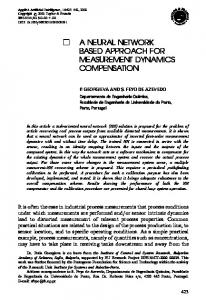
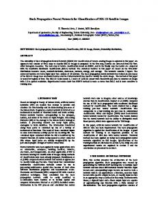
In order to develop the cutting force component model, experimental results were used. The experiments have been carried out with a NC end milling machine and available equipment in our research laboratory. The set up can be seen in figure 1. The three components of cutting force were measured with a piezoelectric dynamometer (Kistler 9255) mounted between the workpiece and the machining table. The force measurements were sampled at 20000 points/second, then digitally low-pass filtered at a cut-off frequency of 250Hz to eliminate the high-frequency components resulting from the machine tool dynamics. The digital data from the A/D board were then acquired and stored by the LabView software into three files for the three force components. The

5

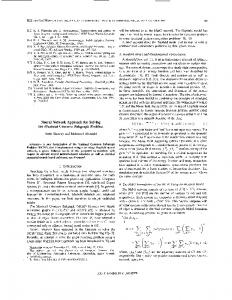
measured force signals were digitized using an A/D converting board at 1 kHz sampling rate for each channel. The data were also displayed on the computer monitor for inspection. The experiments with the end milling cutters were carried out on the NC milling machine (type HELLER BEA1). The spindle is powered by a 6 hp variable speed d.c. motor, programmable for 150 - 3000 r.p.m. Positioning resolution on the machine is 0.005 mm. In experiments five workpiece materials of three different hardness and five diameters of end milling cutters with five different types of interchangeable cutting inserts are used. The table 1 states the ranges of 10 input parameters used by ANN for prediction of cutting force components. The experiments were carried out for all combinations of the chosen input parameters that significantly affect the milling process. These parameters are type of machined material, hardness of the machined material, cutting tool diameter, type of insert, cutting speed, feed, radial and axial depth of cutting, tool wear and the presence of cutting fluid. The coolant RENUS FFM was used for cooling. The cutting tool flank wear was measured with an instrument microscope of 0.01 mm accuracy. A total of 324000 experimental set-ups (tests) were used for developing the ANN predictor. Among them, the settings of cutting speed include vc1 = 12.5m/min, vc2 = 20m/min, vc3 = 25m/min; those of feed rate include f1 = 0.025 mm/tooth, f2 = 0.1 mm/tooth, f3 = 0.2 mm/tooth, f4 = 0.3 mm/tooth; the radial/axial depth of cut is set at RD1 = 1d, RD2 = 0.5d, RD3 = 0.25d ( ’see figure 2’), AD1 = 2mm, AD2 = 4mm, AD3 = 8mm; d - cutter diameter (16 mm); One hundred eight combinations of machining parameters (depth of cut, feedrate, and spindle speed) were selected to make production

6

cuts. Two thirds of 324000 sets of experimental data were used for training the ANN predictor. After the training had been completed another 108000 data were used as testing data. In this way two sets of data groups were generated, one for training and other for estimation tests. The cutting forces values predicted by ANN were compared with measurement values derived from the 108000 data sets in order to determine the error of ANN. Literature on experimental design is numerous and this paper is not intended to cover aspects of experimental design techniques and detailed information can be found in (Benardos and Vosniakos 2002).

[ Insert table 1 about here’]

3. PREDICTIVE CUTTING FORCE MODELING

Artificial neural networks are systems with inputs and outputs composed of many simple interconnected parallel processing elements, called neurons. These systems are inspired by the structure of the brain. Computing with neural networks is nonalgorithmic. They are trained through examples rather than programmed by software. Some of the key features of ANN’s are their processing speed due to their massive parallelism, their proven ability to be trained, to produce instantaneous and correct responses from corrupted inputs once trained, and their ability to generalize information over a wide range. The Multi-Layer BP network is a supervised, continuous valued, multi-input and multi-output feed forward multi-layer network that follows a gradient descent method.

7

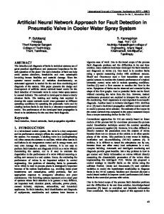
The gradient descent method alters the weight by an amount proportional to the partial derivative of the error with respect to the weight in question. The backpropagation phase of the neural network alters the weights wji so that the error of the network is minimized. This is achieved by taking a pair of input/output vectors and feeding the input vector into the net which generates an output vector, which is compared to the output vector supplied, thus gaining an error value. The error is then passed back through the network (backpropagation process), modifying the weights due to this error using the equations. Hence, if the same sets of input/output vectors are presented to the network, the error would be smaller than previously found. For modeling the cutting force components, three-layer feed-forward neural network was used ( see figure 3’), because this type of neural network which was used gives the most accurate results. The detailed topology of the used ANN with optimal training parameters and mathematical principle of the neuron is shown on figure 3. The ANN were trained with the following parameters: type of machined material, hardness of the machined material, cutting tool diameter, type of insert, cutting speed, feed, radial and axial depth of cutting, tool wear and the presence of the cutting fluid. The first layer of processing elements is the input layer (buffer), where data are presented to the network. The last layer is the output layer (buffer) which holds the network response (cutting forces). The layers between the input and output layers are called hidden layers. The activation of the multilayer feed forward network is obtained by feeding the external input to the first layer, using the corresponding input function to activate the neurons, and then applying the corresponding transfer function to the resulting activations. The vector output of this layer is then fed to the next layer, which is

8

activated in the same way, and so on, until the output layer is activated, giving the network output vector. This is called the feed forward phase, because the activations propagate forward through the layers. The ANN registers the input data only in the numerical form therefore the information about the tool, cutting insert and material must be transformed into numerical code. The type of the cutting insert is indicated with a 8-digit systematization code containing the data on the cutting insert shape, rake angle, free angle, tip radius, base material, cutting insert coating and length of the insert cutting edge.

3.1 Developing the ANN predictor

To develop the optimal neural network predictor the following steps must be accomplished: 1. Experimental preparation-measuring of cutting forces. 2. Preparation of data for training and testing of ANN. Uniting of cutting conditions and measured cutting forces into a data matrix. Breakdown of the data matrix into the input and output vector. Distribution of the input/output vector into the two sets for training and testing. 3. Optimization process - determination the optimal network configuration and training parameters by simulations. 4. Training and testing of ANN. 5. Putting the estimator into operation. Graphic representation of results and prediction of statistic.

9

The described procedure is fully automated although also interactive method of work is possible. In step 3 ( see figure 4’) the model requires manual entering of starting (optimal) training parameters. Figure 4 shows the sequence of steps to be taken when designing the neural cutting force predictor.

3.2 Data Pre-Processing

Training data constitutes a set of input and output vectors. The data is normalized in order to make it suitable for the training process. This was done by mapping each term to a value between 0 and 1 using the Max Min (Szecsi 1999) method. This normalized data was utilized as the inputs (machining conditions) and outputs (components of the cutting force) to train the ANN. In other words, two vectors are formed in order to train the neural network ( see figure 3’): Input vector = [type of machined material, hardness of the machined material, cutting tool diameter, type of insert, cutting speed, feed, radial and axial depth of cutting, tool wear, cutting fluid]. The output vector = [Fx, Fy, Fz].

3.3 Topology of Neural Network and its Adaptation to Cutting Force Modeling Problem

For the BP network, the choice of the training parameters is the most important criteria that determine the degree of success of a network used to perform the specific task. Even if a set of training parameters and a corresponding architecture have been selected and successfully implemented, the question of weather or not the selected parameters

10

are the optimum for that task will still remain to be answered. The important questions are: How many hidden layer neurons, should be assigned to a given network? What values should be picked for the learning rate (a) and momentum rate (b)? The selection of these training parameters is more art than science and is reported to be depended on application. In researches three groups of simulations were executed to study systematically the individual influences of training parameters on the performance of backpropagation networks used for predicting cutting forcers in end milling. The individual effects of varying each of these parameters were kept at (or near) their optimum values. To evaluate the individual effects of training parameters on the performance of neural network 120 different networks were trained, tested and analyzed using actual machining data. The network performances were evaluated using four different criteria: ETstMax, ETst, ETrn, ETrnMax and the number of training cycles.

3.3.1 Defining the number of neurons in the hidden layer The number of neurons in the input and output layer are determined by the number of input and output parameters. The only reason for changing them may be to use different coding schemes. The number of neurons in the hidden layer is a primary parameter of the net architecture. Due to the full interconnection used between neurons, the increase in the number of neurons leads to an increase in net complexity and a decrease in training speed. On the other hand, networks with more neurons in the hidden layer may solve more complex problems. In the first group of simulations the optimum number of neurons in hidden layers was determined in the following way. Fully interconnected networks with tanh transfer

11

function in all their processing elements were used with learning rates fixed at 0.1 and momentum rates fixed at 0.003. The number of neurons in hidden layers was varied between 2 and 20. Five replicates were obtained for each of this 18 network architectures. The average performance during each of the 5 replicates was calculated and recorded.

3.3.2 Defining the learning rate The learning rate primarily affects the training speed. If training of a neural net is required only once, the training speed is not so important. However, future extension of the model with new machining data requires periodical retraining of the network. Basically, the higher the learning rate, the faster the training. However, at too high learning rates, the network may converge to a local minimum instead of the global minimum in the error space. The objective of the next group of simulations was to determine such value of the learning rate with which the error of prediction of ANN would be minimized (ETest). For this purpose fully interconnected networks with tanh transfer function in all their processing elements were trained with the number of hidden layer nodes fixed at the optimum of 15. The momentum rates were also fixed at 0.003. Learning rates were increased in steps of 0.01 staring from 0.1 to 0.5.

3.3.3. Defining the momentum rate To study the effect of momentum rate on performance, a number of backpropagation networks were trained with learning rates fixed at 0.1 while the

12

momentum rate was increased from 0.001 to 0.005, in steps of 0.0005. The number of hidden neurons were fixed at 15. From the results of all simulations the following conclusions can be drawn: • Learning rates below 0.3 give acceptable prediction errors while learning rates must be between 0.01 and 0.2 to minimize the number of training cycles and obtain low predictions errors. Therefore, learning rates that will give an overall optimum performance are any value between 0.01 and 0.2; • To minimize the estimation errors, momentum rates between 0.001 and 0.005 are good. However, the momentum rate should not exceed 0.004 if the number of training cycles is also to be minimized; • The optimum number of hidden layer nodes is 3 or 6. Networks with between 2 and 15 hidden layer nodes, other than 3 or 6, also performed fairly well but resulted in higher training cycles; • Networks trained with the tanh transfer function in all their processing elements give the least prediction errors, while those employing sigmoid and sine give the highest and next highest prediction errors respectively; • Networks that employ the sine function require the lowest number of training cycles followed by the Arctangent, while those that employ the hyperbolic tangent require the highest number of training cycles;

3.4 Training and Testing

Network training involves the process of interactively adjusting the interconnection weights in such a way that the prediction errors on the training set are minimized. The

13

backpropagation algorithm is applied to each pattern set, input and target, for all pattern sets in the training set. Since the learning process is iterative, the entire training set will have to be presented to the network over and over again, until the global error reaches a minimum acceptable value. The basic goal in training any neural network is to minimize the overall error of the network. The Mean Absolute Error (MAE) is given by MAE = ( | y1 - g(x1, W)| + | y1 - g(x1, W)) | + ... + | ym - g(xm, W)| ) / m

(1)

where zm = (xi, yi), i = 1,...,m, is a sequence of m training examples. W is the network weight matrix and g(X, W) is the resulting (vector valued) network function. The training was supervised; the desired outputs (the three maximal cutting force components) of the network also being supplied during training. Training of the ANN was made with raw experimental data of 216000 full training examples. Tanh-type nonlinearities were applied to the neurons. The effect of the following two main training parameters on the training error convergence was also investigated: the learning rate a, controlling the speed of the adaptation of the connection weights between the neurons; and the momentum term β that takes into account the rate of the last change of the connection weights. All of the values of the training parameters were scaled to fit in the normalized range 0-1. After the neural network had been trained it was applied to 108000 examples that did not take part in the training process. This time the solutions of the examples (cutting force components) were not supplied, so that the network had to estimate them. The estimation errors were calculated by means of equation (1)’. It appeared that the Test Set error for the 1450 examples was 4%, slightly higher than the training error (ETrn). Matlab Network Tool Box and Thinks-Pro software were used as a platform to create the networks.

14

In the course of training and testing, neural network computes all of the following statistics: • Training Set error (ETrn). The overall error for the Training Set using the method (MAE) defined by equation (1)’. • Training Set max error (ETrnMax). The largest absolute difference between an actual output and its desired output in the Training Set. • Test Set error (ETst). The overall error for the Test Set using the method (MAE) defined by equation (1)’. • Test Set max error (ETstMax). The largest absolute difference between an actual output and its desired output in the Test Set. Figure 5 shows the uniform falling of the value of all errors (ETst, ETstMax, ETrn, ETrnMax) with the number of iterations during the training and testing process for described network configuration ( see figure 3’). The smallest error of testing (ETst) is reached at iteration 1780. It can be seen in the figure 5 that errors converge not to zero but to 0.04 (4%). This is caused by the presence of some contradicting examples in the training set. The prediction of a network trained with tanh transfer function and optimum parameters of 7-6 hidden nodes, learning rate (0.1) and a momentum rate (0.001) are shown on figure 6. The predictions of a non-optimum networks with nonoptimal parameters are also shown on figure 6.

4. DISCUSSION OF RESULTS

This chapter presents the results of experiments and the comparison and analysis of results between the experimental, analytical (Milfelner and Cus 2003) and ANN model

15

depending on the cutting parameters. An extensive number of tests were made on the milling machine to confirm the neural model with different cutting parameters. Table 3 indicates the results of experiments and prediction of ANN for fourteen randomly selected test conditions ( see table 2’) determined on the basis of the plan of experiments. In all fourteen tests the material Ck 45 with improved machining properties was used. The ball-end milling cutter with interchangeable cutting inserts of type R216-16B20-040 with two cutting edges, of 16 mm diameter and 10° helix angle was selected for machining of the material. The cutting inserts R216-16 03 M-M with 12° rake angle were selected. The cutting insert material is P30-50 coated with TiC/TiN, designated GC 4040. The coolant RENUS FFM was used for cooling. The measured flank wear was 0.15mm in all fourteen tests. The results and/or the values of cutting forces are graphically represented by means of diagrams depending on the angle of rotation of the milling cutter ( see figure 7-8’).

[Insert table 2 about here]

Figure 9(a) shows the results predicted by the BP network and the cutting forces measured in test 1. The test conditions are given in table 2. Figures 9(b) and (c) compare the predicted and measured results for different widths of cut ( see test 7’) and for different depths of cut ( see test 3’), respectively. In figure 9(d), the results for lower feed rates are shown. From the figures it can be seen that the values from prediction coincide well with the values from experiments and in addition, the process of the change of the cutting force with respect to the angle of rotation of the milling cutter and the amplitude agree well, with only slight differences in the peak and valley regions of

16

Fx. The discrepancies are caused by size effects that occur at low uncut chip thicknesses. The slight differences between the simulated and measured results are believed to be caused by the cutter runout, which is evident from the repeated tooth passing patterns in the measured forces. In the cutting test 7, significant vibration between tool and workpiece was observed. For cases with severe tool-workpiece vibration, the effects of vibration should be considered when modeling the cutting forces. The results mutually differ as follows: to 4% for Fx, from 2.7-3.5% for Fy and from 1.4-3.9% for Fz component. Also the comparison of maximum values of the cutting forces from simulation with the experimental values in case of different cutting conditions was made. The maximum force is important in this study due the great significance that this particular variable has in tool breakage. Table 3 lists the maximal predicted and measured forces, and the errors. It shows the effectiveness of the BP network. The maximum percentage prediction cutting force error is found to be less than 8% for all the cases tested. The percentage deviation was defined as %error = (Target-Pred.)/Target x 100. The magnitudes of the errors are relatively small if compared with the forces developed during milling, which in this study vary between 50 and 3500 N.

[Insert table 3 about here]

4.1 Comparison of the Neural Network-Based Model with the Analytical Model

17

Based on the values in the 324000 experimental data, the cutting force components were calculated according to analytical model (Milfelner and Cus 2003). The calculated cutting force components were then compared to the actual forces given in the testing data. The predictive capability of using analytical and neural network approaches are compared using statistics, which showed that neural network predictions for three cutting force components were for 4% closer to the experimental measurements, compared to 11% using analytical method.

5. Conclusion

In this paper, supervised neural networks are used to successfully estimate the forces developed during ball-end milling process. The comparison between the predicted cutting forces and measured cutting forces was made. It can be claimed that the comparison of the results obtained from the neural model and of the experimental results confirms the efficiency and accuracy of the model for predicting the cutting forces. By using a multi-layer perceptron with backpropagation training method, the neural network is trained to an accuracy of ±2% error for all three forces. In testing the model, the three force components in oblique cutting were predicted to an accuracy of ±4%. An effort is made to include as many different machining conditions as possible that influence the cutting process. Extensive experimentation forms the basis of the model developed. The procedure should be used for the fast approximate determination of optimum cutting forces on the machine, when there is not enough time for deep analysis. Due to high speed of processing, low consumption of memory, great

18

robustness, possibility of self-learning and simple incorporation into chips the approach ensures estimation of the cutting forces in real time. It provides a robust representation due to the fault-tolerant nature of neural networks. It provides an automated paradigm for prediction of cutting force components since the proposed approach is easy to computerize. The milling system can be modeled on-line, based on this modified backpropagation ANN. The iteration step size of ANN is adjusted in the iteration process to increase the convergence speed. The milling process can be optimized in real-time by the modified ANN. The simulation and experiments show that the adaptive milling system with the modified backpropagation ANN has a high robustness and global stability, Different architectures of ANN and their prediction capabilities are also studied in the research. Future work could be directed to application of other preference models and neural networks to machining process optimization and extension of the proposed approach to adaptive control of machining operations or on-line adjustment of cutting parameters based on information from sensors.

References Cus, F. and Balic, J.(2000) “Selection of cutting conditions and tool flow in flexible manufacturing system”, The International Journal for Manufacturing Science & Technology, 2, 101-106. Yang, M. and Park, H.(1991) “The Prediction of Cutting Force in Ball-End Milling”, International Journal of Machine Tools Manufacturing, 31, 45-54.

19

Feng, H.Y. and Menq, C.H.(1996) “A Flexible Ball-End Milling System Model for Cutting Force and Machining Error Prediction”, ASME J. Manuf. Sci. Eng., 118, 461469. Yucesan, G. and Altintas, Y.(1996), “Prediction of Ball End Milling Forces”, ASME J. Eng. Ind., 118, 95-103. El Mounayri and H. Spence, A.D. and Elbestawi, M.A.(1998) “Milling Process Simulation-A General Solid Modeller Based Paradigm”, ASME J. Manuf. Sci. Eng., 120, 213-221. Kuo R.J.(2000) “Multi-Sensor Integration For On Line Tool Wear Estimation Through Artifical Neural Networks And Fuzzy Neural Network”, Enginering Application Of Artifical Intelligence, 13, 249-261 Lee, T.S. and Lin, Y.J.(2000) “A 3D Predictive Cutting-Force Model for End Milling of Parts Having Sculptured Surfaces”, International Journal of Advanced Manufacturing Technology, 16, 773-783. Liu, Y. and Wang, C.(1999) “Neural Network Based Adaptive Control and Optimisation in the Milling Process”, International Journal of Advanced Manufacturing Technology, 15, 791-795. Milfelner, M. and Cus, F.(2003) “Simulation of cutting forces in ball-end milling”, Robotics and Computer Integrated Manufuring, 19, 99-106. Szecsi, T.(1999) “Cutting force modeling using artificial neural networks”, Journal of Materials Processing Technology, 92-93, 344-349. Tandon, V. and Mounayri, H.(2001) “A Novel Artificial Neural Networks Force Model for End Milling”, International Journal of Advanced Manufacturing Technology, 18, pp. 693-700.

20

Lee, L.C. and Lee, K.S. and Gran, C.S.(1989) “On the correlation between dynamic cutting force and tool wear”, International Journal of Machine Tools Manufacturing, 29, No. 3, 295-303. Masory, O.(1991) “Monitoring machining processes using multi-sensor readings fused by artificial neural networks”, Journal of Materials processing technology, 28, 231-240. Raj, K.H. and Rahul S.S. and Sanjay S. and Patvardhan, C.(2000) “Modeling of manufacturing processes with ANN’ for intelligent manufacturing”, International Journal of Machine Tools and Manufacture, 40, No 6,851-868. Wen-Tung Chien and Chung-Yi Chou(2001) “The predictive model for machinability of 304 stainless steel”, Journal of Materials Processing Technology, 118, No. 1-3, 442447. Benardos, P.G. and Vosniakos, G.C.(2002) “Prediction of surface roughness in CNC face milling using neural networks and Taguchi' s design of experiments”, Robotics and Computer-Integrated Manufacturing, 18, No. 5-6, 343-354. Tandon, V. and El-Mounayri, H. and Kishawy, H.(2002) “NC end milling optimization using evolutionary computation”, International Journal of Machine Tools and Manufacture, 42, No 5, 595-605. Zuperl, U. and Cus, F. and Milfelner, M.(2005) “Fuzzy control strategy for an adaptive force control in end-milling”, Journal of Materials Processing Technology, 164-165, No. 15,1472-1478. Cus, F. and Balic, J.(2003) “Optimization of cutting process by GA approach”, Robotics and Computer-Integrated Manufacturing, 19, No. 1-2, 113-121.

21

Chen-Huei Hsieh and Jyh-Horng Chou and Ying-Jeng W.(2002) “Optimal predicted fuzzy controller of a constant turning force system with fixed metal removal rate”, Journal of Materials Processing Technology, 123, No. 1, 22-30. D' Orazio, T. and Guaragnella, C. and Leo, M. and Distante, A.(2004) “A new algorithm for ball recognition using circle Hough transform and neural classifier”, Pattern Recognition, 37, No. 3, 393-408. Egmont-Petersen M. and de Ridder D. and Handels H.(2002) “Image processing with neural networks - a review”, Pattern Recognition, 35, No. 10, 2279-2301. Liu, Y. and Zuo, L. and Wang, C.(1999) “Intelligent adaptive control in milling process”, International Journal of Computer Integrated Manufacturing, 12, No. 5, 453460. Zuperl, U. and Cus, F.(2003) “Optimization of cutting conditions during cutting by using neural networks”, Robotics and Computer-Integrated Manufacturing, 19, No. 1-2, 189-199.

22

Table 1. Review of input parameters fz [mm [mm] [mm] /tooth]

Input vector

vc [m/ min]

Flank wear wb [mm]

4

3

5

2

2

0.025

12.5

0.15

0.5d

4

0.1

20

0.2

0.25d

6

0.2

25

0.25

Nr. of discrete values

Values/ Type

RD

AD

3

3

1d

0.3

Type of material

Cutter diameterd [mm]

Type of insert

3

5

4

5

yes

125

Ck45Xm

6

GC4040

no

170

St.52.3

12

GC1025

200

16MnCr5

16

GC3020

0.3

X5CrNi18

20

GC3040

0.35

15CrMo5

Cutting Hardness fluid HB

CT530

Table 2. Cutting conditions in end milling experiment Test

RD [mm]

AD [mm]

fz [mm/tooth]

vc [m/min]

Test

RD [mm]

1

16

8

0.2

25

8

8

2

16

8

0.025

12.5

9

8

3

16

4

0.2

25

10

4

16

4

0.025

12.5

11

5

16

2

0.1

25

6

8

8

0.3

7

8

8

0.025

AD fz vc [mm] [mm/tooth] [m/min] 4

0.3

12.5

2

0.025

25

8

2

0.3

12.5

4

8

0.2

25

12

4

4

0.3

25

25

13

4

4

0.025

12.5

12.5

14

4

2

0.025

12.5

Milling cutter R216-16B20-040 (16mm), cutting insert R216-16 03 M-M GC 4040, material Ck 45, wb=0.15mm

23

Table 3. Comparison of the maximal values of measured and predicted cutting forces Test 1 2 3 4 5 6 7 8 9 10 11 12 13 14

Direction x y z x y z x y z x y z x y z x y z x y z x y z x y z x y z x y z x y z x y z x y z

Measured max. Predicted force [N] max. force [N] 2773.4 2712.11 3007.8 3111.71 2226.6 2139.76 1113.3 1068.77 1386.7 1363.14 664.1 676.05 1621.1 1671.07 2285.2 2263.95 1007.8 1044.75 561.7 552.9 496.1 490.86 254.7 269.63 69.1 69.42 55.1 54.74 27.3 27.33 1113.3 1075.45 2847.7 2807.83 1845.3 1777.024 1095.3 1063.54 2449.2 2378.17 1070.3 1058.53 964.1 947.71 2225.8 2156.80 823.4 818.46 683.6 657.62 1503.9 1454.27 695.3 686.95 308.6 299.03 558.6 539.60 418 406.71 488.3 469.25 1621.1 1601.64 757.8 747.94 492.2 484.81 554.7 551.92 285.2 280.35 285.9 277.60 901.6 885.37 683.6 661.72 173.4 168.89 398.4 386.4 222.7 215.12

Absolute error [N] 61.29 -103.91 86.84 44.53 23.56 -11.95 -49.97 21.25 -36.95 8.8 5.24 -14.93 -0.32 0.36 -0.03 37.85 39.86 68.27 31.76 71.02 11.77 16.38 68.99 4.94 25.97 49.62 8.34 9.56 18.99 11.286 19.0 19.45 9.85 7.38 2.77 4.84 8.29 16.22 21.87 4.50 11.9 7.57

Percentage error [%] 2.2 -3.5 3.9 4 1.7 -1.8 -3.1 0.9 -3.7 1.2 0.5 -2.7 -0.8 0.9 -0.1 3.40 1.4 3.7 2.9 2.9 1.1 1.7 3.1 0.6 3.8 3.3 1.2 3.1 3.4 2.7 3.9 1.2 1.3 1.5 0.5 1.7 2.9 1.8 3.2 2.6 3 3.4

Analyt. [9] model [N]

Absolute error [N]

2406.95

-180.35

2928.71 3395.81 1256.92 1605.80 676.72 1431.43 2161.80 1144.86 530.47 517.02 275.22 68.67 54.28 25.20 1053.19 3081.21 2042.74 1192.78 2718.61 999.66 907.21 2156.80 818.46 657.63 1454.27 686.95 299.03 539.60 406.714 469.25 1601.64 747.95 484.82 551.93 280.35 277.61 885.37 661.72 168.89 386.45 215.12

-155.31 -388.01 -143.62 -219.10 -12.62 189.67 123.40 -137.06 31.23 -20.92 -20.52 0.43 0.82 2.10 60.11 -233.51 -197.44 -97.48 -269.4 70.63 56.88 68.99 4.94 25.97 49.62 8.34 9.56 18.99 11.286 19.04 19.45 9.85 7.38 2.77 4.85 8.29 16.23 21.87 4.51 11.95 7.57

Percentage error [%] 5.6

12.9 8.1

12.9 15.8

1.9 -11.7 -5.4 13.6 -4.1 2.1 3.7 -1.1 -2.1 -7.7 5.40 -8.2 -10.7 -8.9 -11 6.6 5.9 3.1 0.6 3.8 3.3 1.2 3.1 3.4 2.7 3.9 1.2 1.3 1.5 0.5 1.7 2.9 1.8 3.2 2.6 3 3.4

24

1000

Fx Fy

800

Amplifiers

600

Fz

400 200

Dynamometer

0 -200

A/D

-400

Digital signal

Kot zasuka [°]

Computer Analog signal LabView

Figure 1. Experimental set-up

y y Vc

y Vc

Vc x

x RD

x

Figure 2. Realization of milling; RD=1d , RD=0.5d , RD=0.25d

Input layer

Cutting fluid (yes/no)

Hidden layers

Training parameters

Output layer

Hardness HB Type of material

Fx

Cutting tool diam.

a

b

Layer 1

0.11

0.001

Layer 2

0.15

0.003

Layer 3

0.01

0.001

a-learning rate b-momentum constant

Fy

Type of insert

Fz

Cutting speed

X1

Feed

X2

Radial depth of cutting Inputs

Axial depth of cutting Flank wear

X3 Xn

time

Weights

W1 i W2 i Output Yj

W3 i

S W jk Xi

Wn i bias

W b

Activation function (tanh)

Figure 3. Predictive force model topology

25

Step-1

Step-2

Step-3

Step-4

Step-5

Simulations Evaluation of results

Measured cutting forces FX, FY in FZ

Data preparation for ANN training and testing

Selection of the best network architecture and searching for optimum training

Upgrading of the ANN model

Training and testing the ANN

Prediction of cutting forces

parameters Generation of data matrix

Determination of training and testing set

Normalization of data

Developing the ANN model

Result Putting the ANN into operation

Figure 4. Schematic representation of functioning of the described cutting force estimator

26

Figure 5. Decrease of errors during supervised training of neural network

actual results - Fz optimum ANN 45

non-optimim ANN (learning rate-0.4) non-optimim network (TF-Sine)

Cutting force Fz [N]

35

25

15

5

0

0.01

0.02

0.03

0.04

0.05

0.06

0.07

0.08

-5 Time [s]

Figure 6. Prediction of the maximal cutting force component (Fz) using networks trained with optimum and non-optimum parameters

27

60 Fx - M Fy - M Fz - M

40

Fx - ANN Fy - ANN

Cutting forces [N]

Fz - ANN 20

0 0

0.01

0.02

0.03

0.04

0.05

0.06

0.07

0.08

-20

-40

-60 Time [s]

Figure 7. Representation of measured (Fx-M, Fy-M, Fz-M) and predicted (Fx-ANN, FyANN, Fz- ANN) cutting forces (Test 14). Ball-end milling cutter R216-16B20-040, cutting insert R216-16 03 M-M GC 4040, material Ck 45, milling width RD=4 mm, milling depth AD=2 mm, feeding f=0.025 mm/tooth, cutting speed vc=12.5 m/min and wb=0.15mm.

28

600 Fx - M Fy - M

500

Fz - M Fx -ANN

400

Fy - ANN Fz - ANN

Cutting forces [N]

300

200

100

0 0

10

20

30

40

50

60

70

80

90

100

-100

-200

-300

Angular position of the cutting edge [°]

Figure 8. Representation of measured (Fx-M, Fy-M, Fz-M) and predicted (Fx-ANN, FyANN, Fz- ANN) cutting forces (Test 6). Ball-end milling cutter R216-16B20-040, cutting insert R216-16 03 M-M GC 4040, material Ck 45, milling width RD=8 mm, milling depth AD=8 mm, feeding f=0.3 mm/tooth, cutting speed vc=12.5 m/min and wb=0.15mm.

29

3000

700

0.05

0.1

0.15

0.2

0.25

0.3

Cutting forces [N]

Cutting forces [N]

2000

a)

1700

-300 0

F-measured Fx-predicted Fz-predicted Fy-predicted

2500

2700

1000 500 0 -500

F-measured Fx-predicted Fz-predicted Fy-predicted

-1300 -2300

c)

1500

0

0.05

0.15

0.2

0.25

0.3

-1000 -1500

Time [s]

Time [s]

2700

600

b)

2200

0.1

d)

500 400 Cutting forces [N]

Cutting forces [N]

1700 1200 700 200 -300 0

0.05

0.1

0.15

-800 -1300

Time [s]

0.2

0.25

0.3

F-measured Fx-predicted Fz-predicted Fy-predicted

300 200 100 0 -100 0

0.05

0.1

0.15

0.2

0.25

0.3

-200 -300 -400

Fy-predicted Fz-predicted Fx-predicted

Time [s]

Figure 9. Comparison of predicted and measured cutting forces: for: (a) for Test 1; (b) for Test 7; (c) for Test 3; (d) for Test 4.

30