Dynamic System Testing Method and Artificial Neural Networks For Solar Water Heater Long-Term Performance Prediction Soteris Kalogirou and Sofia Panteliou* Department of Mechanical Engineering, Higher Technical Institute, P.O. Box 20423, Nicosia 2152, Cyprus Phone: +357-2-306199, Fax: +357-2-494953 email:
[email protected] *Department of Mechanical Engineering and Aeronautics, University of Patras, Patras 26500 Greece. Phone: +30-61-997206, Fax: +30-61-997207 email:
[email protected] ABSTRACT: The performance of a solar hot water thermosyphon system was tested with the dynamic system method according to Standard ISO/CD/9459.5. The system is of closed circuit type and consists of two flat plate collectors with total aperture area of 2.74 m2 and of a 170 liters hot water storage tank. The system was modeled according to the procedures outlined in the standard with the weather conditions encountered in Rome. The simulations were performed for hot water demand temperatures of 45 and 90°C and volume of daily hot water consumption varying from 127 to 200 liters. These results have been used to train a suitable neural network to perform long-term system performance predictions. A total of 5 complete runs (60 patterns) were available. From these, 12 patterns with data for a whole year were used as a validation set, whereas the rest 48 were used for the training (42 sets) and testing (6 sets) of the network. A multi layer feedforward neural network with three hidden slabs was used. Seven input and four output parameters are used. The input data were leaned with adequate accuracy with correlation coefficients varying from 0.993 to 0.998, for the four output parameters. When unknown data were used to the network, satisfactory results were obtained. The maximum percentage difference between the actual (simulated) and predicted results is 6.3%. These results prove that artificial neural networks can be used successfully for this type of predictions. KEYWORDS: Solar water heaters, Dynamic system testing, Artificial neural networks.
INTRODUCTION There are several methods for testing the performance of solar water heating systems. In the present work the performance of the system was tested with the dynamic system method according to Standard ISO/CD/9459.5 (1997). This method takes into account time varying processes for the performance prediction of the system as well as for the parameter identification. Neural networks are widely accepted as a technology offering an alternative way to tackle complex and ill-defined problems. They can learn from examples, are fault tolerant in the sense that they are able to handle noisy and incomplete data, are able to deal with non-linear problems, and once trained can perform prediction at very high speed. The power of neural networks in modeling complex mappings and in system identification has been demonstrated by Kohonen (1984), Narendra and Parthasarathi (1990), and Ito (1992). This work encouraged many researchers to explore the possibility of using neural network models in real world applications such as in control systems, in classification, and in modeling complex process transformations (Kah et al., 1995; Kreider and Wang, 1995; Curtiss et al., 1995). Artificial neural networks have been used successfully to model a solar steam generator. In particular they have been used to model the collector intercept factor (Kalogirou et al., 1996), the local concentration ratios around the periphery of the collector receiver (Kalogirou, 1996), and the starting-up of the system (Kalogirou et al., 1998). This was a complex problem since the system was modeled during its heat-up, i.e., under transient conditions. Besides, artificial neural networks have been used for the same system to predict the mean monthly steam production with an error confined to less than 5.1% (Kalogirou et al., 1997). Additionally, neural networks have been used successfully to
predict the energy extracted and the water temperature rise of thermosyphon flat-plate solar collector systems (Kalogirou et al., 1999). The aim of this study is to investigate the suitability of neural networks as tools for the estimation of the long-term solar water heating system performance. It is also required to use simple and easily measurable system and environmental data such as total daily radiation and mean air temperature. This would facilitate the work of design engineers in the field.
COLLECTION OF DATA The solar system is of the thermosyphonic type and consists of two flat plate collectors with total aperture area of 2.74m2 and a 170 liters hot water storage tank. The system is of the closed circuit type, i.e., a heat exchanger is installed in between the solar collectors and the hot water storage tank. The system was modeled according to the procedures outlined in the standard ISO/CD/9459.5 with the weather conditions encountered in Rome. The simulations were performed for hot water demand temperatures of 45 and 90°C and volume of daily hot water consumption varying from 127 to 200 liters. The system was modeled for all hours of the year (8760 hours). The program then presents a summary of the results on a monthly basis. These monthly results have been used to train a suitable neural network to perform long-term system performance predictions. A total of 5 complete runs were performed, i.e., 60 patterns were available in total. From the total of 60 sets of data, 12 (data for a whole year) were randomly selected (all of the same run) to be used for validation of the model and the remaining 48 for training and testing the network. A sample of the training data set is shown in Table 1. Table 1. A sample of the training data set. Input parameters N Gt Ta Cs Q 31 130 7.6 6.16 171 28 174 8.0 6.16 196 31 214 10.2 6.16 204 30 238 13.0 6.16 211 31 263 17.2 6.16 214 30 281 21.0 6.16 216 31 261 24.2 6.16 216 31 271 24.0 6.16 216 30 258 21.1 6.16 216 ... ... ... ... ...
Month Td VL 1 45 127 2 45 127 3 45 127 4 45 127 5 45 127 6 45 127 7 45 127 8 45 127 9 45 127 ... ... ... Notes: 1. Td = hot water demand temperature (°C), 2. VL = volume of daily hot water consumption (lt), 3. N = number of days in each month, 4. Gt = mean solar irradiance (W/m2), 5. Ta = mean ambient temperature of the month (°C),
6. 7. 8. 9. 10.
Output parameters f Aa 0.795 1.320 0.907 1.120 0.948 0.957 0.977 0.884 0.993 0.813 1.000 0.768 1.000 0.826 1.000 0.797 1.000 0.835 ... ...
DT 27.8 31.7 33.2 34.2 34.8 35.0 35.0 35.0 35.0 ...
Cs = mean load capacitance rate (W/K), Q = delivered power (W), f = fractional system gain, Aa = average effective solar system area (m2), DT = the mean load temperature difference (°C).
The data used as input to the artificial neural network are the same, with those required by the simulation program supplied with the standard. The only difference is that mains mean cold water temperature and draw-off rate were not used because their values were constant in all cases (Tcw=10°C and Vs=10 lt/min). These data are those that mostly affect the performance of the system and are easily obtainable. These include some system parameters, weather conditions, and the required output. The network is also trained to give an output the same as in the above-mentioned program.
ARTIFICIAL NEURAL NETWORK MODEL Artificial neural networks (ANN) mimic somewhat the learning process of a human brain. Instead of complex rules and mathematical routines, ANN’s are able to learn the key information patterns within a multidimensional information domain. In addition, the inherently noisy data do not seem to cause a problem, since they are neglected.
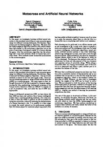
According to Haykin (1994) a neural network is a massively parallel distributed processor that has a natural propensity for storing experiential knowledge and making it available for use. It resembles to the human brain in two respects; the knowledge is acquired by the network through a learning process, and inter-neuron connection strengths, known as synaptic weights, are used to store the knowledge. ANN models represent a new method in system prediction. ANNs operate like a “black box” model, requiring no detailed information about the system. Instead, they learn the relationship between the input parameters and the controlled and uncontrolled variables by studying previously recorded data, similar to the way a non-linear regression might perform. Another advantage of using ANNs is their ability to handle large and complex systems with many interrelated parameters. They seem to simply ignore excess input data that are of minimal significance and concentrate instead on the more important inputs. Various network architectures such as of 3, 4, and 5 layers, a number of recurrent type, and a number of feedforward ones, have been investigated aiming at finding the one that could result in the best overall performance. The architecture, from those tested, that gave the best results and finally adopted is shown in Fig. 1. This is a feedforward architecture, which has three hidden slabs. The architecture adopted in this work has different activation functions in each slab as shown in Fig. 1. Different activation functions are applied to hidden layer slabs in order to detect different features in a pattern processed through a network. The network consists of eight neurons in each hidden slab.
INPUT LAYER SLAB
HIDDEN LAYER SLABS
SLAB 2
OUTPUT LAYER SLAB
(8 neurons) Activation Gaussian
SLAB 4
SLAB 1
(8 neurons)
SLAB 5
(7 neurons)
Activation Gaussian Complement
(4 neurons)
SLAB 3 Activation Linear
(8 neurons)
Activation Logistic
Activation tanh
Figure 1. Neural network architecture employed. Seven input neurons have been used in the input slab, corresponding to the following input parameters: • month of the year, • hot water demand temperature (°C), • volume of daily hot water consumption (lt), • number of days in each month, • mean solar irradiance of the month (W/m2) • mean ambient temperature of the month (°C), and • mean load capacitance rate (W/K).
The same parameters are used as input to the computer simulation program supplied with the standard. The output is a four-element vector corresponding to the values of delivered power (Q in W), fractional system gain (f), average effective solar system area (Aa in m2), and mean load temperature difference (DT in °C). These four parameters are the most important ones to determine the long-term performance of the system. The output parameters are also the same as the ones given by the program supplied with the standard. The back-propagation learning algorithm has been used. The network gain was set to 0.1, and the momentum factor to 0.1 whereas the weights were initialized to a constant value of 0.3. A total of 48 patterns have been collected for the 4 runs of the simulation program as described above. From this set, 42 patterns were used for the training of the network while the remaining 6 patterns were randomly selected to be used as test patterns. The training data were learned with an excellent accuracy. The coefficients of multiple determination (R2-values) and the correlation coefficients obtained are shown in Table 2. The fact that all values are close to unity indicates that the mapping was performed at a satisfactory level. Table 2. Results of the training of the network. Parameter Coefficient of multiple determination (R2-values) Delivered power (W) 0.9950 Fractional system gain 0.9957 Average effective solar system area (m2) 0.9943 Mean load temperature difference (°C) 0.9862
Correlation coefficient 0.998 0.998 0.997 0.993
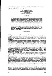
RESULTS / VALIDATION Once a satisfactory degree of input-output mapping has been reached, the network training is frozen and the set of completely unknown test data was applied for verification. The validation data set, shown in Table 3, comprise data for the same system but at different operating conditions, which the network has not seen before. A comparison of the predicted results with the actual (simulated) values for the four output parameters is shown in Figures 2 to 4. As can be seen the accuracy obtained is adequate. In fact, in some cases the two lines are so close that are indistinguishable. The maximum percentage error is 6.3% occurring for the month of November for the delivered power. It should be stressed that the training of the network required about 4 minutes on a Pentium 133 MHz machine. The subsequent predictions for the unknown cases require about 1-2 seconds on the same machine; thus the estimation time was reduced drastically without sacrificing accuracy. Table 3. Validation data set. Input parameters Month Td VL N Gt Ta Cs Q 1 45 170 31 130 7.6 6.16 208 2 45 170 28 174 8.0 6.16 245 3 45 170 31 214 10.2 6.16 264 4 45 170 30 238 13.0 6.16 278 5 45 170 31 263 17.2 6.16 285 6 45 170 30 281 21.0 6.16 289 7 45 170 31 261 24.2 6.16 289 8 45 170 31 271 24.0 6.16 288 9 45 170 30 258 21.1 6.16 288 10 45 170 31 181 16.0 6.16 280 11 45 170 30 145 12.4 6.16 248 12 45 170 31 90 8.4 6.16 154 Note: For explanation of symbols refer to Table 1.
Output parameters F Aa 0.722 1.60 0.850 1.41 0.915 1.24 0.963 1.17 0.987 1.08 1.000 1.03 1.000 1.11 0.999 1.07 0.999 1.12 0.972 1.55 0.859 1.71 0.533 1.71
DT 25.3 29.7 32.0 33.7 34.5 35.0 35.0 35.0 34.9 34.0 30.1 18.7
CONCLUSIONS The objective of this work was to predict the long-term performance of a solar water heating thermosyphon system tested with the dynamic system method using artificial neural networks. The system consists of two flat plate collectors and a hot water storage tank of closed circuit type.
The system was modeled according to the procedures outlined in the standard with the weather conditions encountered in Rome. The simulations were performed for hot water demand temperatures of 45 and 90°C and volume of daily hot water consumption varying from 127 to 200 liters. The system was modeled for all months of the year. These results have been used to train a suitable neural network to perform long-term system performance predictions. A total of 5 complete runs were available, i.e., 60 patterns were available in total. From these, 12 patterns with data for a whole year were used as a validation set, whereas the rest 48 were used for the training (42 sets) and testing (6 sets) of the network.
Delivered power (W)
350 300 250 200 150 100
Actual Q Netw ork Q
50 0 Jan Feb Mar Apr May Jun Jul Aug Sep Oct Nov Dec
Month
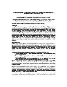
Actual f Actual Aa Netw ork f Netw ork Aa
2 1.5 1
2 1.5 1
0.5
0.5
0
Effective area (m2)
Fractional system gain
Figure 2. Comparison of actual (simulated) data with ANN predicted data for delivered power.
0 Jan Feb Mar Apr May Jun Jul Aug Sep Oct Nov Dec Month
Load temp. difference (°C)
Figure 3. Comparison of actual (simulated) data with ANN predicted data for fractional system gain and effective solar system area.
40.0 35.0 30.0 25.0 20.0 15.0 10.0 5.0 0.0
Actual DT Netw ork DT
Jan Feb Mar Apr May Jun
Jul Aug Sep Oct Nov Dec
Month
Figure 4. Comparison of actual (simulated) data with ANN predicted data for mean load temperature difference.
A multi layer feedforward neural network with three hidden slabs was used. The input parameters are the same to those used as input to the simulation program. The output is also similar to the output given by the program. The input data were leaned with adequate accuracy. The obtained correlation coefficients were varying from 0.993 to 0.998, for the four output parameters, which are very adequate. When unknown data were used to the network, satisfactory results were obtained, with correlation coefficients of the same order of magnitude as above. The maximum percentage difference between the actual (simulated) and predicted results is 6.3%. These results prove that artificial neural networks can be used successfully for this type of predictions. We are planing to apply artificial neural networks and the dynamic system testing method for a number of systems in order to create an assessment tool for this type of solar systems. ACKNOWLEDGEMENT: All the data used in the present work have been obtained from the senior project thesis of Mrs. Eleni Vosnou titled “Comparison of testing methods for the evaluation of solar domestic heating systems”, Athens Polytechnic, 1997. The authors would also like to thank Dr. Theotokis Pafelias for providing the above thesis.
REFERENCES Curtiss P.S., Brandemuehl, M.J. and Kreider J.F., 1995, “Energy Management in Central HVAC Plants using Neural Networks”. In Haberl J.S., Nelson R.M. and Culp C.C. (Eds.). The use of Artificial Intelligence in Building Systems. ASHRAE. pp. 199 - 216. Haykin S., 1994, “Neural Networks: A Comprehensive Foundation”, Macmillan, New York. ISO/CD/9459.5, 1997, “Solar Heating-Domestic Water Heating Systems: Part 5: System Performance by Means of Whole System Testing and Computer Simulation”. Kah A.H., San Q.Y., Guan S.C., Kiat W.C. and Koh Y.C., 1995, “Smart Air-Conditioning System Using Multilayer Perceptron Neural Network with a Modular Approach”. Proceedings of the IEEE International Conference ICNN’95, Perth, Western Australia, Vol. 5, pp. 2314-2319. Kalogirou S.A., 1996, “Artificial Neural Networks for Predicting the Local Concentration Ratio of Parabolic Trough Collectors”. Proceedings of the International Conference EuroSun’96, Freiburg, Germany, pp. 470-475. Kalogirou S.A., Neocleous C.C and Schizas C.N., 1996, “A Comparative Study of Methods for Estimating Intercept Factor of Parabolic Trough Collectors”. Proceedings of the International Conference EANN’96, London, UK, pp. 5-8. Kalogirou S.A., Neocleous C.C and Schizas C.N., 1997, “Artificial Neural Networks for the Estimation of the Performance of a Parabolic Trough Collector Steam Generation System”. Proceedings of the International Conference EANN’97, Stockholm, Sweden, pp. 227-232. Kalogirou S.A., Neocleous C.C and Schizas C.N., 1998, “Artificial Neural Networks in Modeling the Starting-up of a Solar Steam Generation Plant”. Applied Energy, Vol. 60, No. 2, pp.89-100. Kalogirou, S., Panteliou, S. and Dentsoras, A., 1999,. “Modelling of Solar Domestic Water Heating Systems Using Artificial Neural Networks”. Paper accepted for publication in Solar Energy Journal. Kohonen T., 1984,. “Self-Organization and Associative Memories”. Berlin-Verlag. Kreider J.F. and Wang X.A., 1995, “Artificial Neural Network Demonstration for Automated Generation of Energy Use Predictors for Commercial Buildings”. In Haberl, J.S., Nelson, R.M. and Culp, C.C. (Eds.). The use of Artificial Intelligence in Building Systems. ASHRAE. pp. 193-198. Ito Y., 1992,. “Approximation of Functions on a Compact Set by Finite Sums of a Sigmoid Function with and without Scaling”. Neural Networks, Vol. 4, pp. 817-826. Narendra K.S. and Parthasarathi K., 1990, “Identification and Control of Dynamical Systems Using Neural Networks”. IEEE Transactions on Neural Networks, Vol. 1, pp. 4-27.