May 4, 2016 - AbstractâThis paper studies real-time scheduling of mixed- criticality ... case execution time (WCET) estimation for high-criticality tasks. On the ...
EDF-VD Scheduling of Mixed-Criticality Systems with Degraded Quality Guarantees Di Liu1 , Jelena Spasic1 Gang Chen2 , Nan Guan3 , Songran Liu2 , Todor Stefanov1 , Wang Yi2, 4 1
arXiv:1605.01302v1 [cs.OH] 4 May 2016
Leiden University, The Netherlands 2 Northeastern University, China 3 Hong Kong Polytechnic University, Hong Kong 4 Uppsala University, Sweden
Abstract—This paper studies real-time scheduling of mixedcriticality systems where low-criticality tasks are still guaranteed some service in the high-criticality mode, with reduced execution budgets. First, we present a utilization-based schedulability test for such systems under EDF-VD scheduling. Second, we quantify the suboptimality of EDF-VD (with our test condition) in terms of speedup factors. In general, the speedup factor is a function with respect to the ratio between the amount of resource required by different types of tasks in different criticality modes, and reaches 4/3 in the worst case. Furthermore, we show that the proposed utilization-based schedulability test and speedup factor results apply to the elastic mixed-criticality model as well. Experiments show effectiveness of our proposed method and confirm the theoretical suboptimality results.
I. I NTRODUCTION An important trend in real-time embedded systems is to integrate applications with different criticality levels into a shared platform in order to reduce resource cost and energy consumption. To ensure the correctness of a mixed-criticality (MC) system, highly critical tasks are subject to certification by Certification Authorities under extremely rigorous and pessimistic assumptions [1]. This generally causes large worstcase execution time (WCET) estimation for high-criticality tasks. On the other hand, the system designer needs to consider the timing requirement of the entire system, but under less conservative assumptions. The challenge in scheduling MC systems is to simultaneously guarantee the timing correctness of (1) only high-criticality tasks under very pessimistic assumptions, and (2) all tasks, including low-critical ones, under less pessimistic assumptions. The scheduling problem of MC systems has been intensively studied in recent years (see Section II for a brief review). In most of previous works, the timing correctness of highcriticality tasks are guaranteed in the worst case scenario at the expense of low-criticality tasks. More specifically, when any high criticality task executes for longer than its low-criticality WCET (and thus the system enters the high-criticality mode), all low-criticality tasks will be completely discarded and the resource are all dedicated for meeting the timing constraints of high-criticality tasks [2]–[5]. However, such an approach seriously disturbs the service of low-criticality tasks. This is not acceptable in many practical problems, especially for control systems where the performance of controllers mainly depends on the execution frequency of control tasks [6].
To overcome this problem, Burns and Baruah in [7] introduced an MC task model where low-criticality tasks reduce their execution budgets such that low-criticality tasks are guaranteed to be scheduled in high-criticality mode with regular execution frequency (i.e., the same period) but degraded quality1 . Since the idea of reducing execution budgets to keep tasks running is conceptually similar to the imprecise computation model [8] [9], in this paper we call an MC system with possibly reduced execution budgets of low criticality tasks an imprecise mixed criticality (IMC) system. In [7], the authors consider preemptive fixed-priority scheduling for the IMC system model and extend the adaptive mixed criticality (AMC) [3] approach to provide a schedulability test for the IMC model. In this paper, we study the EDF-VD scheduling of IMC systems. EDF-VD is designed for the classical MC system model, in which EDF is enhanced by deadline adjustment mechanisms to compromise the resource requirement on different criticality levels. EDFVD has shown strong competence by both theoretical and empirical evaluations [2], [4], [5]. For example, [2] proves that EDF-VD is a speedup-optimal MC scheduling and in [4], [5] experimental evaluations show that EDF-VD outperforms other MC scheduling algorithms in terms of acceptance ratio. The main technical contributions of this paper include • •
•
We propose a sufficient test for the IMC model under EDF-VD, - see Theorem 3 in Section IV; For the IMC model under EDF-VD, we derive a speedup factor function with respect to the utilization ratios of high criticality tasks and low criticality tasks - see Theorem 4 in Section V. The derived speedup factor function enables us to quantify the suboptimality of EDF-VD and evaluate the impact of the utilization ratios on the speedup factor. We also compute the maximum value 4/3 of the speedup factor function, which is equal to the speedup factor bound for the classical MC model [2]. With extensive experiments, we show that for the IMC model, by using our proposed sufficient test, in most cases EDF-VD outperforms AMC [7] in terms of the number of schedulable task sets. Moreover, the experimental results validate the observations we obtained for speedup factor.
1 In [8] [9], the output quality of a task is related to its execution time. The longer a task executes, the better quality results it produces.
Moreover, the schedulability test and speedup factor results of this paper also apply to the elastic mixed-criticality (EMC) model proposed in [6], where the periods of low-criticality tasks are scaled up in high-criticality mode, see in Section VI. The remainder of this paper is organized as follows: Section II discusses the related work. Section III gives the preliminaries and describes the IMC task model and its execution semantics. Section IV presents our sufficient test for the IMC model and Section V derives the speedup factor function for the IMC under EDF-VD. Section VI extends the proposed sufficient test to the EMC model. Finally, Section VII shows our experimental results and Section VIII concludes this paper. II. R ELATED W ORK Burns and Davis in [10] give a comprehensive review of work on real-time scheduling for MC systems. Many of these literatures, e.g., [2] [4] [5], consider the classical MC model in which all low criticality tasks are discarded if the system switches to the high criticality mode. In [7], Burns and Baruah discuss three approaches to keep some low criticality tasks running in high-criticality mode. The first approach is to change the priority of low criticality tasks. However, for fixedpriority scheduling, deprioritizing low criticality tasks cannot guarantee the execution of the low criticality tasks with a short deadline after the mode switches. [7]. Similarly, for EDF, lowering priority of low criticality tasks leads to a degraded service [11]. In this paper, we consider the IMC model which improves the schedulability of low criticality tasks in highcriticality mode by reducing their execution time. The IMC model can guarantee the regular service of a system by trading off the quality of the produced results. For some applications given in [8] [9] [12], such trade-off is preferred. The second approach in [7] is to extend the periods of low criticality tasks when the system mode changes to high-criticality mode such that the low criticality tasks execute less frequently to ensure their schedulability. Su et al. [6] [13] and Jan et al. [14] both consider this model. However, some applications might prefer an on-time result with a degraded quality rather than a delayed result with a perfect quality. Some example applications can be seen in [15] [8] [9]. Then, the approach of extending periods is less useful for this kind of applications. The last approach proposed in [7] is to reduce the execution budget of low criticality tasks when the system mode switches, i.e., the use of the IMC model studied in this paper. In [7], the authors extend the AMC [3] approach to test the schedulability of an IMC task set under fixed-priority scheduling. However, the schedulability problem for an IMC task set under EDF-VD [2], has not yet been addressed. Therefore, in this paper, we study the schedulability of the IMC task model under EDF-VD and propose a sufficient test for it. III. P RELIMINARIES This section first introduces the IMC task model and its execution semantics. Then, we give a brief explanation for EDFVD scheduling [2] and an example to illustrate the execution semantics of the IMC model under EDF-VD scheduling.
A. Imprecise Mixed-Criticality Task Model We use the implicit-deadline sporadic task model given in [7] where a task set γ includes n tasks which are scheduled on a uniprocessor. Without loss of generality, all tasks in γ are assumed to start at time 0. Each task τi in γ generates an infinite sequence of jobs {Ji1 , Ji2 ...} and is characterized by τi = {Ti , Di , Li , Ci }: • Ti is the period or the minimal separation interval between two consecutive jobs; • Di denotes the relative task deadline, where Di = Ti ; • Li ∈ {LO, HI} denotes the criticality (low or high) of a task. In this paper, like in many previous research works [6] [11] [2] [4] [5], we consider a duel-criticality MC model. Then, we split tasks into two task sets, γLO = {τi |Li = LO} and γHI = {τi |Li = HI}; LO HI LO • Ci = {Ci , Ci } is a list of WCETs, where Ci and HI Ci represent the WCET in low-criticality mode and the WCET in high-criticality mode, respectively. For a highcriticality task, it has CiLO ≤ CiHI , whereas CiLO ≥ CiHI for a low-criticality task, i.e., low-criticality task τi has a reduced WCET in high-criticality mode. Then each job Ji is characterized by Ji = {ai , di , Li , Ci }, where ai is the absolute release time and di is the absolute deadline. Note that if low-criticality task τi has CiHI = 0, it will be immediately discarded at the time of the switch to high-criticality mode. In this case, the IMC model behaves like the classical MC model. The utilization of a task is used to denote the ratio between its WCET and its period. We define the following utilizations for an IMC task set γ: • •
∀τi ∈γLO •
∀τi ∈γLO
For all high-criticality tasks, we have total utilizations X X LO HI UHI = uLO uHI i , UHI = i ∀τi ∈γHI
•
C HI
C LO
= Ti i ; For every task τi , it has uLO = Ti i , uHI i i For all low-criticality tasks, we have total utilizations X X LO HI ULO = uLO uHI i , ULO = i
∀τi ∈γHI
For an IMC task set, we have LO LO U LO = ULO + UHI ,
HI HI U HI = ULO + UHI
B. Execution Semantics of the IMC Model The execution semantics of the IMC model are similar to those of the classical MC model. The major difference occurs after a system switches to high-criticality mode. Instead of discarding all low-criticality tasks, as it is done in the classical MC model, the IMC model tries to schedule low-criticality tasks with their reduced execution times CiHI . The execution semantics of the IMC model are summarized as follows: • The system starts in low-criticality mode, and remains in this mode as long as no high-criticality job overruns its low-criticality WCET CiLO . If any job of a low-criticality task tries to execute beyond its CiLO , the system will suspend it and launch a new job at the next period;
Task τ1 τ2
L LO HI
CiLO 4 4
CiHI 2 7
Ti 9 10
ˆi D
Deadline miss
7
0
Table I: Illustrative example
5
10
15 Switch
0
5
10
15
d1
t2
high-criticality mode τ1 only has execution budget of 2 , i.e., C1HI , τ1 executes one unit and suspends. Then, τ2 completes its left execution 4 (C2HI − C2LO ) before its deadline.
18
τ2 20
Figure 1: Scheduling of Example I If any job of high-criticality task executes for its CiLO time units without signaling completion, the system immediately switches to high-criticality mode; • As the system switches to high-criticality mode, if jobs of low-criticality tasks have completed execution for more than their CiHI but less than their CiLO , the jobs will be suspended till the tasks release new jobs for the next period. However, if jobs of low-criticality tasks have not completed their CiHI (≤ CiLO ) by the switch time instant, the jobs will complete the left execution to CiHI after the switch time instant and before their deadlines. Hereafter, all jobs are scheduled using CiHI . For highcriticality tasks, if their jobs have not completed their CiLO (≤ CiHI ) by the switch time instant, all jobs will continue to be scheduled to complete CiHI . After that, all jobs are scheduled using CiHI . Santy et al. [16] have shown that the system can switch back from the high-criticality mode to the low-criticality mode when there is an idle period and no high-criticality job awaits for execution. For the IMC model, we can use the same scenario to trigger the switch-back. In this paper, we focus on the switch from low-criticality mode to high-criticality mode. C. EDF-VD Scheduling The challenge to schedule MC tasks with EDF scheduling algorithm [17] is to deal with the overrun of high-criticality tasks when the system switches from low-criticality mode to high-criticality mode. Baruah et al. in [2] proposed to artificially tighten deadlines of jobs of high-criticality tasks in low-criticality mode such that the system can preserve execution budgets for the high-criticality tasks across mode switches. This approach is called EDF with virtual deadlines (EDF-VD). D. An Illustrative Example Here, we give a simple example to illustrate the execution semantics of the IMC model under EDF-VD. Table I gives two tasks, one low-criticality task τ1 and one high-criticality task τ2 , where Dˆi is the virtual deadline. Figure 1 depicts the scheduling of the given IMC task set, where we assume that the mode switch occurs in the second period of τ2 . When the system switches to high-criticality mode, τ2 will be scheduled by its original deadline 10 instead of its virtual deadline 7. Hence, τ1 preempts τ2 at the switch time instant. Since in •
t1
Figure 2: The defined time instants
τ1 0
a1
IV. S CHEDULABILITY A NALYSIS In [7], an AMC-based schedulability test for the IMC model under fixed priority scheduling has been proposed. However, to date, a schedulability test for the IMC model under EDF-VD has not been addressed yet. Therefore, inspired by the work in [2] for the classical MC model, we propose a sufficient test for the IMC model under EDF-VD. A. Low Criticality Mode We first ensure the schedulability of tasks when they are in low-criticality mode. As the task model is in low-criticality mode, the tasks can be considered as traditional real-time tasks scheduled by EDF with virtual deadlines (VD). The following theorem is given in [2] for tasks scheduled in low-criticality mode. Theorem 1 (Theorem 1 from [2]). The following condition is sufficient for ensuring that EDF-VD successfully schedules all tasks in low-criticality mode: x≥
LO UHI LO 1 − ULO
(1)
where x ∈ (0, 1) is used to uniformly modify the relative deadline of high-criticality tasks. Since the IMC model behaves as the classical MC model in low-criticality mode, Theorem 1 holds for the IMC model as well. B. High Criticality Mode For high-criticality mode, the classical MC model discards all low-criticality jobs after the switch to high-criticality mode. In contrast, the IMC model keeps low-criticality jobs running but with degraded quality, i.e., a shorter execution time. So the schedulability condition in [2] does not work for the IMC model in the high-criticality mode. Thus, we need a new test for the IMC model in high-criticality mode. To derive the sufficient test in high-criticality mode, suppose that there is a time interval [0, t2 ], where a first deadline miss occurs at t2 and t1 denotes the time instant of the switch to high-criticality mode in the time interval, where t1 < t2 . Assume that J is the minimal set of jobs generated from task set γ which leads to the first deadline miss at t2 . The minimality of J means that removing any job in J guarantees the schedulability of the rest of J . Here, we introduce some notations for our later interpretation. Let variable ηi denote the cumulative execution time of task τi in the interval [0, t2 ]. J1 denotes a special high-criticality job which has switch time instant t1 within its period (a1 , d1 ), i.e, a1 < t1 < d1 .
Furthermore, J1 is the job with the earliest release time amongst all high-criticality jobs in J which execute in [t1 , t2 ). Figure 2 visualizes the defined time instants. Moreover, we define a special type of job for low-criticality tasks which is useful for our later proofs.
and with its cumulative execution time equal to (di − ai )uLO i HI uLO > u has its deadline d ≤ (a + x(t − a )). i 1 2 1 i i With the propositions and notations given above, we derive an upper bound of the cumulative execution time ηi of lowcriticality task τi .
Definition 1. A job Ji from low-criticality task τi is a carryover job, if its absolute release time ai is before and its absolute deadline di is after the switch time instant, i.e., ai < t1 < di .
Lemma 1. For any low-criticality task τi , it has
With the notations introduced above, we have the following propositions, Proposition 1 (Fact 1 from [2]). All jobs in J that execute in [t1 , t2 ) have deadline ≤ t2 . It is easy to observe that only jobs which have deadlines ≤ t2 are possible to cause a deadline miss at t2 . If a job has its deadline > t2 and is still in set J , it will contradict the minimality of J . Proposition 2. The switch time instant t1 has t1 < (a1 + x(t2 − a1 ))
(2)
ηi ≤ (a1 + x(t2 − a1 ))uLO + (1 − x)(t2 − a1 )uHI i i
Proof: If uLO = uHI i i , it is trivial to see that Lemma 1 > uHI holds. Below we focus on the case when uLO i . If a i system switches to high-criticality mode at t1 , then we know that low-criticality tasks are scheduled using CiLO before t1 and using CiHI after t1 . To prove this lemma, we need to consider two cases, where τi releases a job within interval (a1 , t2 ] or it does not. We prove the two cases separately. Case A (task τi releases a job within interval (a1 , t2 ]): There are two sub-cases to be considered. • Sub-case 1 (No carry-over job): The deadline of a job of low-criticality task τi coincides with switch time instant t1 . The cumulative execution time of low-criticality task τi within time interval [0, t2 ] can be bounded as follows, ηi ≤ (t1 − 0) · uLO + (t2 − t1 ) · uHI i i
Proof: Let us consider a time instant (a1 + x(d1 − a1 )) which is the virtual deadline of job J1 . Since J1 executes in time interval [t1 , t2 ), its virtual deadline (a1 + x(d1 − a1 )) must be greater than the switch time instant t1 . Otherwise, it should have completed its low-criticality execution before t1 , and this contradicts that it executes in [t1 , t2 ). Thus, it holds that t1 < (a1 + x(d1 − a1 )) ⇒t1 < (a1 + x(t2 − a1 ))
Since t1 < (a1 + x(t2 − a1 )) according to Proposition 2 and for low-criticality task τi it has uLO > uHI i i , then � �� ηi < a1 + x(t2 − a1 ) uLO + t2 − a1 + x(t2 − a1 ) uHI i i ⇔ηi < (a1 + x(t2 − a1 ))uLO + (1 − x)(t2 − a1 )uHI i i •
(since d1 ≤ t2 )
Proposition 3. If a carry-over job Ji has its cumulative execution equal to (di − ai )uLO and uLO > uHI i i i , its deadline di is ≤ (a1 + x(t2 − a1 )). Proof: For a carry-over job Ji , if it has its cumulative execution equal to (di − ai )uLO and uLO > uHI i i i , it should complete its CiLO execution before t1 . Otherwise, if job Ji has executed time units Ci ∈ [CiHI , CiLO ) at time instant t1 , it will be suspended and will not execute after t1 . Now, we will show that when job Ji completes its CiLO execution, its deadline is di ≤ (a1 + x(t2 − a1 )). We prove this by contradiction. First, we suppose that Ji has its deadline di > (a1 + x(t2 − a1 )) and release time ai . As shown above, job Ji completes its CiLO execution before t1 . Let us assume a time instant t∗ as the latest time instant at which this carryover job Ji starts to execute before t1 . This means that at this time instant all jobs in J with deadline ≤ (a1 + x(t2 − a1 )) have finished their executions. This indicates that these jobs will not have any execution within interval [t∗ , t2 ]. Therefore, jobs in J with release time at or after time instant t∗ can form a smaller job set which causes a deadline miss at t2 . Then, it contradicts the minimality of J . Thus, carry-over job Ji
(3)
Sub-case 2 (with carry-over job): In this case, before the carry-over job, jobs of τi are scheduled with its CiLO . After the carry-over job, jobs of τi are scheduled with its CiHI . It is trivial to observe that for a carry-over job its maximum cumulative execution time can be obtained when it completes its CiLO within its period [ai , di ], i.e., (di − ai )uLO i . Considering the maximum cumulative execution for the carry-over job, we then have for lowcriticality task τi , ηi ≤ (ai − 0)uLO + (di − ai )uLO + (t2 − di )uHI i i i ⇔ηi ≤ di uLO + (t2 − di )uHI i i Proposition 3 shows as Ji has its cumulative execution equal to (di − ai ) · uLO i , it has di ≤ (a1 + x(t2 − a1 )). HI Given uLO > u for low-criticality task, we have i i ηi ≤ di uLO + (t2 − di )uHI i i � �� ⇒ηi ≤ a1 + x(t2 − a1 ) uLO + t2 − a1 + x(t2 − a1 ) uHI i i ⇔ηi ≤ (a1 + x(t2 − a1 ))uLO + (1 − x)(t2 − a1 )uHI i i
Case B (task τi does not release a job within interval (a1 , t2 ]): In this case, let Ji denote the last release job of task τi before a1 and ai and di are its absolute release time and absolute deadline, respectively. If di ≤ t1 , we have ηi = (ai − 0)uLO + (di − ai ) · uLO = di uLO i i i
If di > t1 , Ji is a carry-over job. As we discussed above, the maximum cumulative execution time of carry-over job Ji is (di − ai )uLO i , so we have ηi ≤ (ai − 0)uLO + (di − ai ) · uLO ⇔ ηi ≤ di uLO i i i Similarly, according to Proposition 3, we obtain,
Since time instant t2 is the first deadline miss, it means that there is no idle time instant within interval [0, t2 ]. Note that if there is an idle instant, jobs from set J which have release time at or after the latest idle instant can form a smaller job set causing deadline miss at t2 which contradicts the minimality of J . Then, we obtain �
ηi ≤ di · uLO ≤ (a1 + x(t2 − a1 ))uLO i i
N=
�� ⇒ηi < (a1 + x(t2 − a1 ))uLO + t2 − a1 + x(t2 − a1 ) uHI i i
Proposition 4 (Fact 3 from [2]). For any high-criticality task τi , it holds that a1 + (t2 − a1 )uHI (4) ηi ≤ uLO i x i Proposition 4 is used to bound the cumulative execution of the high-criticality tasks. Since in the IMC model the highcriticality tasks are scheduled as in the classical MC model, Proposition 4 holds for the IMC model as well. With Lemma 1 and Proposition 4, we can derive the sufficient test for the IMC model in high-criticality mode. Theorem 2. The following condition is sufficient for ensuring that EDF-VD successfully schedules all tasks in highcriticality mode:
�
∀τi ∈γHI
� a1 + x(t2 − a1 ) uLO + (1 − x)(t2 − a1 )uHI i i
�
∀τi ∈γLO
+
X ∀τi ∈γHI
�
a1 LO ui + (t2 − a1 )uHI i x
�
LO HI ⇔N ≤ (a1 + x(t2 − a1 ))ULO + (1 − x)(t2 − a1 )ULO a1 LO HI + UHI + (t2 − a1 )UHI x U LO LO LO ⇔N ≤ a1 (ULO + HI ) + x(t2 − a1 )ULO x HI HI + (1 − x)(t2 − a1 )ULO + (t2 − a1 )UHI
LO HI HI ⇔xULO + (1 − x)ULO + UHI >1
By taking the contrapositive, we derive the sufficient test for the IMC model when it is in high-criticality mode: LO HI HI xULO + (1 − x)ULO + UHI ≤1
HI Note that if ULO = 0, i.e., no low-criticality tasks are scheduled after the system switches to high-criticality mode, our Theorem 2 is the same as the sufficient test (Theorem 2 in [2]) for the classical MC model in high-criticality mode. Hence, our Theorem 2 actually is a generalized schedulability condition for (I)MC tasks under EDF-VD. By combining Theorem 1 (see Section IV-A) and our Theorem 2, we prove the following theorem,
Theorem 3. Given an IMC task set, if HI LO UHI + ULO ≤1
HI HI LO ) + ULO 1 − (UHI UHI ≤ HI LO LO − ULO 1 − ULO ULO
Since the tasks must be schedulable in low-criticality mode, the condition given in Theorem 1 holds and we have 1 ≥ U LO LO (ULO + HI x ). Hence, HI HI + (1 − x)(t2 − a1 )ULO + (t2 − a1 )UHI
(8)
(7)
(9)
where HI HI LO LO HI UHI + ULO < 1 and ULO < 1 and ULO > ULO
(10)
then this IMC task set can be scheduled by EDF-VD with a deadline scaling factor x arbitrarily chosen in the following range � � LO HI HI UHI 1 − (UHI + ULO ) x∈ , LO LO − U HI 1 − ULO ULO LO Proof: Total utilization U ≤ 1 is the exact test for EDF on a uniprocessor system. If the condition in (8) is met, the given task set is worst-case reservation [2] schedulable under EDF, i.e., the task set can be scheduled by EDF without deadline scaling for high-criticality tasks and execution budget reduction for low-criticality tasks. Now, we prove the second condition given by (9). From Theorem 1, we have,
(6)
LO N ≤a1 + x(t2 − a1 )ULO
> t2
∀τi ∈γHI
then the IMC task set is schedulable by EDF; otherwise, if
By using Lemma 1 and Proposition 4, N is bounded as follows X
ηi
LO HI HI ⇔x(t2 − a1 )ULO + (1 − x)(t2 − a1 )ULO + (t2 − a1 )UHI > t2 − a1
(5)
Proof: Let N denote the cumulative execution time of all tasks in γ = γLO ∪ γHI over interval [0, t2 ]. We have X X N= ηi + ηi
N≤
�
X
LO HI HI ⇒a1 + x(t2 − a1 )ULO + (1 − x)(t2 − a1 )ULO + (t2 − a1 )UHI > t2
Lemma 1 gives the upper bound of the cumulative execution time of a low-criticality task in high-criticality mode. In order to derive the sufficient test for the IMC model in highcriticality mode, we need to upper bound the cumulative execution time of high-criticality tasks.
∀τi ∈γLO
ηi +
∀τi ∈γLO
⇔ηi < (a1 + x(t2 − a1 ))uLO + (1 − x)(t2 − a1 )uHI i i
LO HI HI xULO + (1 − x)ULO + UHI ≤1
X
x≥
LO UHI LO 1 − ULO
From Theorem 2, we have LO HI HI xULO + (1 − x)ULO + UHI ≤1
⇔x ≤
HI HI 1 − (UHI + ULO ) LO HI ULO − ULO
U LO
1−(U HI +U HI )
HI HI LO Therefore, if 1−U ≤ , the schedulability LO LO −U HI ULO LO LO conditions of both Theorem 1 and 2 are satisfied. Thus, the IMC tasks are schedulable under EDF-VD.
V. S PEEDUP FACTOR The speedup factor bound is a useful metric to compare the worst-case performance of different MC scheduling algorithms. The speedup factor bound for the classical MC model under EDF-VD [2] has been shown to be 4/3. The following is the definition of the speedup factor for an MC scheduling algorithm.
(a) plane 1
(b) plane 2
(c) vertical surface
Definition 2 (from [2]). An algorithm A has a speedup factor f ≥ 1, if any task system that is schedulable on a unitspeed processor by using a hypothetical optimal clairvoyant scheduling algorithm2 , can be successfully scheduled on a speed-f processor by algorithm A. For notational simplicity, we define HI UHI = c,
LO UHI =α×c
LO ULO
HI ULO
= b,
(d) Feasible solution space
=λ×b
Figure 3: 3D space of optimization problem (13)
where α ∈ (0, 1] and λ ∈ [0, 1]. α denotes the utilization ratio LO HI between UHI and UHI , while λ denotes the utilization ratio HI LO between ULO and ULO . First, let us analyze the speedup factor of two corner cases. HI LO , this means that there is = UHI When α = 1, i.e., UHI no mode-switch. Therefore, the task set is scheduled by the LO + traditional EDF, i.e., the task set is schedulable if ULO LO UHI ≤ 1. Since EDF is the optimal scheduling algorithm on a uniprocessor system, the speedup factor is 1. When λ = 1, i.e., HI LO , if the task set is schedulable in high-criticality = ULO ULO LO HI ≤ 1 by Theorem 2. Then it is + ULO mode, it must hold UHI scheduled by the traditional EDF and thus the speedup factor is 1 as well. In this paper, instead of generating a single speedup factor bound, we derive a speedup factor function with respect to (α, λ). This speedup factor function enables us to quantify the suboptimality of EDF-VD for the IMC model in terms of speedup factor (by our proposed sufficient test) and evaluate the impact of the utilization ratio on the schedulability of an IMC task set under EDF-VD. First, we strive to find a minimum speed s (≤1) for a clairvoyant optimal MC scheduling algorithm such that any implicit-deadline IMC task set which is schedulable by the clairvoyant optimal MC scheduling algorithm on a speed-s processor can satisfy the schedulability test given in Theorem 3, i.e., schedulable under EDF-VD on a unit-speed processor. Lemma 2. Given b, c ∈ [0, 1], α ∈ (0, 1), λ ∈ [0, 1), and max{b + αc, λb + c} ≤ S(α, λ)
(11)
where
√ (1 − αλ)((2 − αλ − α) + (λ − 1) 4α − 3α2 ) S(α, λ) = 2(1 − α)(αλ − αλ2 − α + 1)
2 A ‘clairvoyant’ scheduling algorithm knows all run-time information, e.g., when the mode switch will occur, prior to run-time.
then it guarantees αc 1 − (c + λb) ≤ (12) 1−b b − λb Proof: Suppose that s ≥ max{b + αc, λb + c}. We strive to find a minimal value s to guarantee that (12) in Theorem 3 is always satisfied. Based on this, we construct an optimization problem as follows, minimize s
(13)
subject to b + αc ≤ s
(14)
λb + c ≤ s
(15)
2
λb + (αλ − α + 1)bc − (λ + 1)b − c + 1 ≤ 0 (16) 0 ≤ b ≤ 1,
0≤c≤1
(17)
where α and λ are constant and s, b, c are variables. If we can prove that S(α, λ) is the optimal solution of the optimization problem (13), then Lemma 2 is proved. Below, we prove that S(α, λ) is the optimal solution of the optimization problem (13)3 . Each of constraints in the optimization problem (13) defines a feasible space in the three-dimension space. In Figure 3(a), the space above the plane is a feasible space satisfying constraint (14), where the plane corresponds to b + αc = s. For constraint (15), λb + c = s draws a plane and the feasible space is above the plane shown in Figure 3(b). Similarly, when constraint (16) makes its right-hand-side equal to the left-hand-side, we draw a vertical curved surface seen in Figure 3(c) and the space outside the vertical surface is the feasible space4 . As a result, 3 This optimization problem is a non-convex problem and thus we cannot use general convex optimization techniques such as the Karush-Kuhn-Tucker (KKT) approach [18] to solve it. 4 As the arrows direct.
This function covers all points which are on the vertical surface and one plane and at same time satisfy all constraints. By doing some calculus, we know that Eq. (18) is monotonically decreasing in (0, b0 ] and monotonically increasing in (b0 , 1]. Therefore, the minimal value of Eq. (18) can be obtained at (b0 , c0 , s0 ). The complete proof is given by Lemma 4 in Appendix I. It means that we can obtain the optimal solution of optimization problem (13) by solving the following equation system. b0 + xc0 = s0 λb0 + c0 = s0 2 λb0 +(αλ−α+1)b0 c0 −(λ+1)b0 −c0 +1 = 0 By joining the first two equations we have c0 = and applying it to the last equation in (19) gives
1.333
0.0 0.2 0.4
λ
1−λ 1−α
× b0 ,
(−αλ2 + αλ − α + 1)b20 + (αλ + α − 2)b0 + (1 − α) = 0 By the well-known Quadratic Formula we get the two roots of the above quadratic equation. √ (2 − αλ − α) + (1 − λ) −3α2 + 4α 1 b0 = (20) 2(−αλ2 + αλ − α + 1) √ (2 − αλ − α) − (1 − λ) −3α2 + 4α b20 = (21) 2(−αλ2 + αλ − α + 1) We can prove that b20 is larger than 1 and thus should be dropped (since we require 0 ≤ b ≤ 1), while b10 is in the range of [0, 1]. The detailed proof is given by Lemma 5 in Appendix I. As a result, we obtain the optimal solution 1 1−αλ 1 (b10 , 1−α 1−λ b0 , 1−λ b0 ) for Eq. (19). Thus, we have
0.6
0.8
1.0 0.0
0.2
0.4
0.6
0.8
1.0
α
Figure 4: 3D image of speedup factor w.r.t α and λ α λ 0 0.1 0.3 0.5 0.7 0.9 1
0.1
0.3
1/3
0.5
0.7
0.9
1
1.254 1.231 1.183 1.134 1.082 1.028 1
1.332 1.308 1.256 1.195 1.126 1.046 1
1.333 1.310 1.259 1.200 1.130 1.048 1
1.309 1.293 1.254 1.206 1.143 1.056 1
1.227 1.219 1.201 1.174 1.133 1.061 1
1.091 1.090 1.087 1.083 1.074 1.048 1
1 1 1 1 1 1 1
Table II: Speedup factor w.r.t α and λ
1 − αλ 1 b0 1−λ √ (1 − αλ)((2 − αλ − α) + (λ − 1) 4α − 3α2 ) = 2(1 − α)(αλ − αλ2 − α + 1)
S(α, λ) =
Therefore, Lemma 2 is proved. Lemma 2 shows that any IMC task set which is schedulable by an optimal clairvoyant MC scheduling algorithm on a speed-S(α, λ) is also schedulable on a unit-speed processor by EDF-VD. As a direct result, we have the following theorem, Theorem 4. The speedup factor of EDF-VD with IMC task sets is upper bounded by f=
(19)
1.35 1.30 1.25 1.20 1.15 1.10 1.05
speedup factor
the feasible solutions subject to these three constraints must be above both planes and outside the vertical curved surfaces. Below we will prove the minimum value of s in the feasible solution space must be on the vertical surface and one plane. First assume that we have a point (b00 , c00 , s00 ) which satisfies all constraints but is not on the vertical surface. If we connect the origin (0, 0, 0) and (b00 , c00 , s00 ), this line must have an intersection point (b∗0 , c∗0 , s∗0 ) with the vertical surface. It is easy to observe that s∗0 < s00 - see in Figure 3(d). This means that any point which is not on the vertical surface can find a point with smaller value of s on the vertical surface which satisfies all constraints. Therefore, the point with the minimal s must be on the vertical surface. Similarly, the minimal s must be on one of the two planes. Otherwise, if it is not on any plane, we always can find a projected point on one plane which has a smaller value of s. We have shown above that to obtain the minimal value of s the point must be on the vertical surface and one plane. Then, the two planes have an intersection line and this line intersects with the vertical surface at a point denoted by (b0 , c0 , s0 ). By taking constraints (14)(15) and (16), we formulate a piece-wise function of s with respect to b as follows. ( (αλ2 −αλ)b2 +b−1 0 < b ≤ b0 (αλ−α+1)b−1 (18) s(b) = (1−α)b2 +(αλ+α−1)b−α b0 < b ≤ 1 (αλ−α+1)b−1
2(1 − α)(αλ − αλ2 − α + 1) √ (1 − αλ)((2 − αλ − α) + (λ − 1) 4α − 3α2 )
The speedup factor is shown to be a function with respect to α and λ. Figure 4 plots the 3D image of this function and Table II lists some of the values with different α and λ. By doing some calculus, we obtain the maximum value 1.333, i.e., 4/3, of the speedup factor function when λ = 0 and α = 13 , which is highlighted in Figure 4 and Table II. We see that the speedup factor bound is achieved when the task set is a classical MC task set. From Figure 4 and Table II, we observe different trends for the speedup factor with respect to α and λ. • First, given a fixed λ, the speedup factor is not a monotonic function with respect to α. The relation between α and the speedup factor draws a downward parabola. Therefore, a straightforward conclusion regarding the impact of α on the speedup factor cannot be drawn. • Given a fixed α, the speedup factor is a monotonic decreasing function with respect to increasing λ. It is seen that increasing λ leads to a smaller value of the speedup
factor. This means that a larger λ brings a positive effect on the schedulability of an IMC task set.
miss at t2 . This contradicts the minimality of J . Therefore, in this case we have di ≤ (a1 + x(t2 − a1 ))
VI. E XTENSION TO E LASTIC M IXED -C RITICALITY M ODEL Su and Zhu in [6] introduced an Elastic Mixed-Criticality (EMC) task model, where the elastic model [19] is used to model low criticality tasks. When the MC system switches to high criticality mode, low-criticality tasks scale up their original period to a larger period such that low-criticality tasks continue to be scheduled with a degraded service (less frequently). Although the EMC model has been studied by [6] [13] [14], there is not a utilization-based sufficient test for the EMC model. Therefore, in this section, we prove that the theories proposed in Section IV apply to the EMC model [6] as well. Here, we use Timax (≥ Ti ) to denote the extended period of a low-criticality task τi . Since, in the EMC model, the WCETs of a low-criticality tasks are the same in two modes, the utilization of low-criticality task τi in high-criticality mode is computed as uHI = CiLO /Timax . i
Lemma 3. Lemma 1 still holds for low-criticality tasks of the EMC model in high-criticality mode.
Proposition 5 (Lemma 1 from [6]). A set of EMC tasks is HI HI ≤ 1. + ULO EMC schedulable under EDF-VD if UHI
By Proposition 6, we replace di with (a1 + x(t2 − a1 )) in Eq. (29)
HI to Here, in order to keep the consistence, we use ULO denote U (L, min) in [6]. Proposition 5 is provided in [6] to check the schedulability of an EMC task set on a uniprocessor. However, Proposition 5 is a necessary test. This means that even if a given task set satisfies the condition presented in Proposition 5, it is still possible that the task set is unschedulable under EDF-VD. Below, we prove that the theories proposed in Section IV can apply to the EMC model. First, in low-criticality mode, since the EMC model just behaves like the classical MC model, Theorem 1 holds for the EMC model. Then we discuss the schedulability of the EMC model in high-criticality mode. We have the following definition for the carry-over job of a low criticality task in the EMC model:
Definition 3. In the EMC model, carry-over job Ji of low criticality task τi has its release time ai < t1 and original deadline di > t1 . Then, we prove the following proposition for a carry-over job. Proposition 6. For an EMC carry-over job Ji , if it completes its execution before switch time instant t1 , then its original deadline di is ≤ (a1 + x(t2 − a1 )). Proof: Consider that carry-over job Ji completes its execution before switch time instant t1 . Suppose that Ji has its original deadline di > (a1 + x(t2 − a1 )). Let t∗ denote the latest time instant at which Ji starts to execute before t1 . At time instant t∗ , all jobs in J with deadlines ≤ (a1 +x(t2 −a1 )) then have finished their execution. Therefore, these jobs do not have any execution within interval [t∗ , t2 ]. This implies that jobs in J which are released at or after t∗ can form a smaller job set and this smaller job set is sufficient to cause deadline
Proof: We can prove this lemma by doing some modifications on the proof of Lemma 1. Here, we mainly focus on the modified part. The proof uses the same notations explained in Section IV. For the EMC model, we need to consider a special case when carry-over job Ji of low-criticality task τi has its > t2 . Since t2 is a deadline miss, extended deadline dmax i a job with deadline > t2 will not be scheduled within [t1 , t2 ) -see Proposition 1. If dmax > t2 , job Ji will not be executed i after the switch time instant t1 and the maximum cumulative execution time of τi can be obtained as job Ji completes its CiLO before t1 . Hence, the cumulative execution of task τi can be bounded by, ηi ≤ ai · uLO + (di − ai )uLO = di · uLO i i i
(22)
ηi ≤ (a1 + x(t2 − a1 ))uLO + (t2 − (a1 + x(t2 − a1 )))uHI i i ⇔ηi ≤ (a1 + x(t2 − a1 ))uLO + (1 − x)(t2 − a1 )uHI i i (23)
The rest of the proof can follow the proof of Lemma 1. A complete proof can be found in Appendix II. Lemma 3 shows that Lemma 1 can still bound the cumulative execution time of low-criticality tasks of the EMC model in high-criticality mode. Moreover, since there is no difference how the high-criticality tasks are scheduled in the EMC model or in the classical MC model, Proposition 4 still holds for the high-criticality tasks in the EMC model. As a result, Theorem 2 holds for the EMC model as well. Then, we can directly obtain the following theorem, Theorem 5. Theorem 3 is a sufficient test for the EMC model under EDF-VD. Since Theorem 3 is a sufficient test for the EMC model under EDF-VD, the speedup factor results we obtained in Section V also apply to the EMC model, i.e., the speedup factor bound of the EMC model under EDF-VD is also 4/3 by using our proposed sufficient test. VII. E XPERIMENTAL E VALUATION In this section, we conduct experiments to evaluate the effectiveness of the proposed sufficient test for the IMC model in terms of schedulable task sets (acceptance ratio). Moreover, we conduct experiments to verify the observations obtained in Section V regarding the impact of α and λ on the average acceptance ratio. Our experiments are based on randomly generated MC tasks. We use a task generation approach, similar to that used in [5] [4], to randomly generate IMC task sets to evaluate the proposed sufficient test. Each task τi is generated based on the following procedure,
• •
• •
•
pCriticality is the probability that the generated task is a high-criticality task; pCriticality∈ [0, 1]. Period Ti is randomly selected from range [100, 1000]. In order to have sufficient number of tasks in a task set, utilization ui is randomly drawn from the range[0.05, 0.2]. For any task τi , CiLO = ui ∗ Ti . R ≥ 1 denotes the ratio CiHI /CiLO for every highcriticality task. If Li = HI, we set CiHI = R ∗ CiLO . It is easy to see that α used in the speedup factor function is equal to R1 ; λ ∈ (0, 1] denotes the ratio CiHI /CiLO for every lowcriticality task. If Li = LO, we set CiHI = λ ∗ CiLO .
In the experiment, we generate IMC task sets with different target utilization U . Each task set is generated as follows. Given a target utilization U , we first initialize an empty task set. Then, we generate task τi according to the task generation procedure introduced above and add the generated task to the task set. The task set generation stops as we have U − 0.05 ≤ Uavg ≤ U + 0.05 where Uavg =
U LO + U HI 2
is the average total utilization of the generated task set. If adding a new task makes Uavg > U + 0.05, then the added task will be removed and a new task will be generated and added to the task set till the condition is met. A. Comparison with AMC [7] To date, the modified AMC given in [7] is the only related work considering the schedulability of the IMC model under fixed-priority scheduling. Therefore, in the first experiment, we compare EDF-VD by using our proposed test to the AMC approach in [7] in terms of average acceptance ratio. In this experiment, R is randomly selected from a uniform distribution [1.5, 2.5]. With different λ and pCriticality settings, we vary Uavg from 0.4 to 0.95 with step of 0.05, to evaluate the effectiveness of the proposed sufficient test in terms of the average acceptance ratios. We generate 10,000 task sets for each given Uavg . Due to space limitations, we only present the experimental results when pCriticality= 0.5. Results with different pCriticality settings can be found in Appendix III. The results are shown in Figure 5, where the x-axis denotes the varying Uavg and the y-axis denotes the acceptance ratio. In the figures, let EDF-VD and AMC denote our proposed schedulability test and the one proposed in [7], respectively. In most cases, EDF-VD outperforms AMC in terms of acceptance ratio. We observe the following trends: 1) When Uavg ∈ [0.5, 0.8], EDF-VD always outperforms AMC in terms of acceptance ratio. However, if Uavg > 0.8 and λ = 0.3 or 0.5, AMC performs better than EDFVD. The same trend is also found for the classical MC model under EDF-VD and AMC, see the comparison in [4].
1.0 Acceptance ratio
•
0.8 Uavg =0.65 Uavg =0.70 Uavg =0.75 Uavg =0.80 Uavg =0.85
0.6 0.4 0.2 0.00.2 0.3 0.4 0.5 0.6 0.7 0.8 λ
Figure 6: Impact of λ
2) By comparing sub-figures in Figure 5, we see that the average acceptance ratio improves when λ increases. This confirms the observation for the speedup factor we obtained in Section V. The increasing λ leads to a smaller speedup factor. As a result, it provides a better schedulability. We need to notice that when λ increases, not only EDF-VD improves its acceptance ratio but the acceptance ratio of AMC [7] also improves. B. Impact of α and λ Above, we compare our proposed sufficient test to the existing AMC approach. In this section, we conduct experiments to further evaluate the impact of λ and α (1/R) on the acceptance ratio. In this experiment, we select Uavg = {0.65, 0.7, 0.75, 0.8, 0.85} to conduct experiments. We fix Uavg to a certain utilization and vary λ and α to evaluate the impact. We first show the results for λ. The results are depicted in Figure 6, where the x-axis denotes the value of λ from 0.2 to 0.9 with step of 0.1 and the y-axis denotes the average acceptance ratio. R is randomly selected from a uniform distribution [1.5, 2.5] and pCriticality= 0.5. Similarly, 10,000 task sets are generated for each point in the figures. A clear trend can be observed that the acceptance ratio increases as λ increases. This trend confirms the positive impact of increasing λ on the schedulability which we have observed in Section V. Next we conduct experiments to evaluate the impact of α on the schedulability. Similarly, we fix Uavg and vary α to carry out the experiments. Due to α = R1 , if α is given, we compute the corresponding R to generate task sets. The results are depicted in Figure 7, where λ = 0.5. The xaxis denotes the varying α from 0.1 to 0.9 with step of 0.1. while the y-axis denotes the average acceptance ratio. First, from Table II, we see that with increasing α the speedup factor first increases till a point. This means within this range the scheduling performance of EDF-VD gradually decreases. After that point, the speedup factor decreases which means the scheduling performance of EDF-VD gradually improves. The experimental results confirm what we have observed for α in Section V. The acceptance ratio gradually decreases till a point and then it increases.
1.0
0.8
0.8
0.8
0.6 0.4
AMC EDF-VD
0.2 0.00.4
0.5
0.6
0.7
Uavg
0.8
0.9
Acceptance ratio
1.0 Acceptance ratio
Acceptance ratio
1.0
0.6 0.4
AMC EDF-VD
0.2 0.00.4
0.5
(a) λ = 0.3
0.6
0.7
Uavg
0.8
0.9
0.6 0.4
AMC EDF-VD
0.2 0.00.4
0.5
(b) λ = 0.5
0.6
0.7
Uavg
0.8
0.9
(c) λ = 0.7
Acceptance ratio
Figure 5: Varying Uavg with different λ and pcriticality=0.5
1.0 0.9 0.8 0.7 0.6 0.5 0.4 0.3 0.2 0.10.1 0.2 0.3 0.4 0.5 0.6 0.7 0.8
[4]
Uavg =0.65 Uavg =0.70 Uavg =0.75 Uavg =0.80 Uavg =0.85
α
[5]
[6] [7] [8]
Figure 7: Impact of α [9] [10]
VIII. C ONCLUSIONS In this paper, the imprecise mixed-criticality (IMC) model from [7] is investigated. A sufficient test for the IMC model under EDF-VD is proposed and the proposed sufficient test later applies to the EMC model as well. Based on the proposed sufficient test, we derive a speedup factor function with respect to the utilization ratio α of all high-criticality tasks and the utilization ratio λ of all low-criticality tasks. This speedup factor function provides a good insight to observe the impact of α and λ on the speedup factor and quantifies suboptimality of EDF-VD for the IMC/EMC model in terms of speedup factor. Our experimental results show that our proposed sufficient test outperforms the AMC approach in terms of acceptance ratio. Moreover, the extensive experiments also confirm the observations we obtained for the speedup factor.
[11]
[12] [13]
[14]
[15] [16]
R EFERENCES [1] S. Baruah, H. Li, and L. Stougie, “Towards the design of certifiable mixed-criticality systems,” in Proceedings of the 16th IEEE RealTime and Embedded Technology and Applications Symposium (RTAS). Washington, DC, USA: IEEE Computer Society, 2010, pp. 13–22. [2] S. Baruah, V. Bonifaci, G. D’Angelo, H. Li, A. Marchetti-Spaccamela, S. V. der Ster, and L. Stougie, “The preemptive uniprocessor scheduling of mixed-criticality implicit-deadline sporadic task systems,” in Proceedings of the 24th Euromicro Conference on Real-Time Systems (ECRTS), July 2012, pp. 145–154. [3] S. K. Baruah, A. Burns, and R. I. Davis, “Response-time analysis for mixed criticality systems,” in Proceedings of the 32nd IEEE Real-Time
[17] [18] [19]
Systems Symposium. Washington, DC, USA: IEEE Computer Society, 2011, pp. 34–43. P. Ekberg and W. Yi, “Bounding and shaping the demand of generalized mixed-criticality sporadic task systems,” Real-time systems, vol. 50, no. 1, pp. 48–86, 2014. A. Easwaran, “Demand-based scheduling of mixed-criticality sporadic tasks on one processor,” in Proceedings of the 2013 IEEE 34th Real-Time Systems Symposium (RTSS). Washington, DC, USA: IEEE Computer Society, 2013, pp. 78–87. H. Su and D. Zhu, “An elastic mixed-criticality task model and its scheduling algorithm,” in Design, Automation Test in Europe Conference Exhibition (DATE), 2013, March 2013, pp. 147–152. A. Burns and S. Baruah, “Towards a more practical model for mixed criticality systems,” in Proceedings of Workshop on Mixed Criticality, IEEE Real-Time Systems Symposium (RTSS), 2013, pp. 1–6. J. W. Liu, K.-J. Lin, W.-K. Shih, A. C.-s. Yu, J.-Y. Chung, and W. Zhao, “Algorithms for scheduling imprecise computations,” Computer, vol. 24, no. 5, pp. 58–68, 1991. J. W. Liu, W.-K. Shih, K.-J. Lin, R. Bettati, and J.-Y. Chung, “Imprecise computations,” Proceedings of the IEEE, vol. 82, no. 1, pp. 83–94, 1994. A. Burns and R. Davis, “Mixed criticality systems-a review,” University of York, Tech. Rep, 2015. P. Huang, G. Giannopoulou, N. Stoimenov, and L. Thiele, “Service adaptions for mixed-criticality systems,” in Proceedings of the 19th Asia and South Pacific Design Automation Conference (ASP-DAC), Jan 2014, pp. 125–130. R. Ravindran, C. M. Krishna, I. Koren, and Z. Koren, “Scheduling imprecise task graphs for real-time applications,” International Journal of Embedded Systems (IJES), vol. 6, 2014. H. Su, N. Guan, and D. Zhu, “Service guarantee exploration for mixedcriticality systems,” in Proceedings of IEEE 20th International Conference on Embedded and Real-Time Computing Systems and Applications (RTCSA), 2014. M. Jan, L. Zaourar, and M. Pitel, “Maximizing the execution rate of lowcriticality tasks in mixed criticality system,” Proceedings of Workshop on Mixed-Criticality, IEEE Real-Time Systems Symposium, pp. 43–48, 2013. J.-Y. Chung, J. W. S. Liu, and K.-J. Lin, “Scheduling periodic jobs that allow imprecise results,” IEEE Trans. Comput., vol. 39, no. 9, pp. 1156–1174, Sep. 1990. F. Santy, L. George, P. Thierry, and J. Goossens, “Relaxing mixedcriticality scheduling strictness for task sets scheduled with fp,” in Proceedings of the 24th Euromicro Conference on Real-Time Systems (ECRTS), July 2012. C. L. Liu and J. W. Layland, “Scheduling algorithms for multiprogramming in a hard-real-time environment,” Journal of the ACM (JACM), 1973. H. W. Kuhn and A. W. Tucker, “Nonlinear programming,” in Proceedings of the Second Berkeley Symposium on Mathematical Statistics and Probability. Berkeley, Calif.: University of California Press, 1951. G. C. Buttazzo, G. Lipari, M. Caccamo, and L. Abeni, “Elastic scheduling for flexible workload management,” IEEE Trans. Comput., vol. 51, no. 3, pp. 289–302, Mar. 2002.
A PPENDIX I Lemma 4. The minimum value of piece-wise function (18) given in Section V is obtained when b = b0 . ( (αλ2 −αλ)b2 +b−1 0 < b ≤ b0 (αλ−α+1)b−1 s(b) = (24) (1−α)b2 +(αλ+α−1)b−α b0 < b ≤ 1 (αλ−α+1)b−1 Proof: For case of 0 < b ≤ b0 , its derivative is s0 (b) =
α(λ − 1)(λ(αy − α + 1)b2 − 2λb + 1) ((αλ − α + 1)b − 1)2
The denominator is obviously positive. For the numerator, since the discriminant of λ(αλ − α + 1)b2 − 2λb + 1 = 0 is (2λ)2 − 4λ(αλ − λ + 1), which is negative since 0 < λ < 1, so we know λ(αλ − α + 1)b2 − 2λb + 1 > 0. Moreover, we have λ − 1 < 0, so putting them together we know the numerator is negative. In summary, s0 (b) is negative and thus s(b) is monotonically decreasing with respect to b in the range b ∈ (0, b0 ]. For case of b0 < b ≤ 1, we can compute the derivative of s(b) by s0 (b) =
(1 − λ)((λy − x + 1)b2 − 2b − (λy − x − 1)) ((λy − x + 1)b − 1)2
The denominator is obviously positive. For the numerator, we focus on (xλ−x+1)b2 −2b−(xλ−x−1) part. The following equation (xλ − x + 1)b2 − 2b − (xλ − x − 1) = 0 1+(x−xλ) has two roots b1 = 1 and b2 = 1−(x−xλ) , which is greater than 1, so we know (xλ−x+1)b2 −2b−(xλ−x−1) is either always positive or always negative in the range of b ∈ (b0 , 1). Since we can construct (xλ − x + 1)b2 − 2b − (xλ − x − 1) > 0 with x = λ = b = 0.5, so we know (xλ−x+1)b2 −2b−(xλ−x−1) is always positive. Moreover, since 1 − x > 0, the numerator of s0 (b) is positive, so overall s0 (b) is positive, and thus s(b) is monotonically increasing with respect to b in the range of b ∈ (b0 , 1]. In summary, we have proved s(b) is monotonically decreasing in (0, b0 ], and monotonically increasing in (b0 , 1], both with respect to b, so the smallest value of s(b) must occur at b0 .
Lemma 5. If 0 < α < 1 and 0 ≤ λ < 1, then √ (2 − αλ − α) + (1 − λ) −3α2 + 4α 1 b0 = >1 2(−αλ2 + αλ − α + 1) √ (2 − αλ − α) − (1 − λ) −3α2 + 4α ∈ [0, 1] b20 = 2(−αλ2 + αλ − α + 1)
(25) (26)
Proof: We start with proving b10 > 1. We first prove b10 ≥ 0 by showing both the numerator and dominator are positive. For simplicity, we use N1 and M1 to denote the numerator and denominator of b10 in (25), and N2 and M2 the numerator and denominator of b20 in (26). Note that the following reasoning relies on that α ∈ (0, 1), λ ∈ [0, 1).
1) N1 > 0. First, we have N1 × N2 = (2 − αλ − α)2 − (1 − λ)2 (−3α2 + 4α) = 4αλ(1 − λ)(1 − α) + 4(1 − α)2 >0 Moreover, it is easy to see N2 > 0. Therefore, we can conclude that N1 is also positive. 2) M1 > 0. 2(−αλ2 +αλ−α+1) = 2(αλ(1−λ)+(1−α)), which is positive. In summary, both the numerator and the denominator of b10 in (25) are positive, so b10 ≥ 0. Next we prove b10 ≤ 1 by showing N1 − M1 ≤ 0: N1 − M 1 p = (λ − 1)( −3α2 + 4α + α(2λ − 1)) which is negative if λ ≥ 0.5 (since λ − 1 < 0 and √ −3α2 + 4α + α(2λ − 1) ≥ 0). So in the following we focus on the case of λ < 0.5. Since λ < 0.5, we know α(2λ − 1) is negative, so we define two positive number A and B as follows p A = −3α2 + 4α (27) B = α(1 − 2λ)
(28)
so N1 − M1 = (λ − 1)(A − B). Since λ − 1 < 0, we only need to prove A − B > 0, which is equivalent to proving A2 − B 2 > 0 (as both A and B are positive): A2 − B 2 > 0, which is done as follows: A2 − B 2 = − 3α2 + 4α − α2 (2λ − 1)2 =4α(1 − α) + 4α2 λ(1 − λ) >0 so we have A−B > 0 and thus N1 −M1 = (λ−1)(A−B) < 0. In summary, we have proved N1 − M1 < 0 for the cases of both λ ≥ 0.5 and λ < 0.5, so we know b10 ∈ [0, 1]. Next we prove b20 > 1, by showing N2 − M2 > 0 N2 − M 2 p = (1 − λ)( −3α2 + 4α − α(2λ − 1)) √ If λ ≤ 0.5, then −3α2 + 4α − α(2λ − 1) > 0, and since 1 − λ > 0 we have N2 − M2 > 0. If λ > 0.5, we let C = α(2λ − 1) > 0 and also use A as defined above, N2 − M2 = (1 − λ)(A − C). To prove A − C > 0, it suffices to prove A2 − C 2 > 0, as shown in the following: A2 − C 2 = − 3α2 + 4α − α2 (2λ − 1)2 = 4α − (3 + (2λ − 1)2 )α2 > 4α − 4α2 (λ < 1 ,so 2λ − 1 < 1) >0 By now we have proved N2 − M2 for both cases of λ ≤ 0.5 and λ > 0.5, so we known b20 > 1.
1.0
0.8
0.8
0.8
0.6 0.4
AMC EDF-VD
0.2 0.00.4
0.5
0.6
0.7
Uavg
0.8
0.9
Acceptance ratio
1.0 Acceptance ratio
Acceptance ratio
1.0
0.6 0.4
AMC EDF-VD
0.2 0.00.4
0.5
(a) λ = 0.3
0.6
0.7
Uavg
0.8
0.6 0.4
AMC EDF-VD
0.2 0.00.4
0.9
0.5
(b) λ = 0.5
0.6
0.7
0.8
Uavg
0.9
(c) λ = 0.7
Figure 8: Varying UB with different λ and pcriticality=0.3
A PPENDIX II The following is the complete proof of Lemma 3. Proof: We use the same notations explained in Section IV. = uHI When uLO i , it is trivial to see that Lemma 1 holds for i the EMC model. Now we focus on the case when uLO > uHI i i To prove this case, we need to consider two cases where lowcriticality task τi releases a job within interval (a1 , t2 ] or it does not. • Case 1 (τi releases a job within interval (a1 , t2 ]): If there is no carry-over job , the proof is the same as we have proved for the IMC model (see the proof of Sub-case 1 in Lemma 1). Here, we focus on the case that there is a carry-over job. Let Ji denote the carry-over job with absolute release time ai , original deadline di , and maximum deadline dmax . Here, we consider two cases, i dmax > t2 and dmax ≤ t2 . i i – dmax > t2 : since t2 is a deadline miss, a job with i deadline > t2 will not be scheduled within [t1 , t2 ) -see Proposition 1. If dmax > t2 , job Ji will not i be executed after the switch time instant t1 and the maximum cumulative execution time of τi can be obtained as job Ji completes its CiLO before t1 . Hence, the cumulative execution of task τi can be bounded by, ηi ≤ ai · uLO + (di − ai )uLO = di · uLO i i i
•
For di > t1 , if dmax ≤ t2 , then the maximum cumulative i execution can be bounded as follows: ηi ≤ ai · uLO + (dmax − ai )uHI i i i ⇒ηi ≤ ai · uLO + (t2 − ai )uHI i i
ηi ≤ (a1 + x(t2 − a1 ))uLO + (t2 − (a1 + x(t2 − a1 )))uHI i i ⇔ηi ≤ (a1 + x(t2 − a1 ))uLO + (1 − x)(t2 − a1 )uHI i i (33)
dmax i
If > t2 , our reasoning is similar to the case discussed in Case 1. The maximum cumulative execution happens to that Ji completes its execution before t1 . Similarly, in this case, its cumulative execution can be upper bounded by ηi ≤ ai uLO + (di − ai )uLO i i
By Proposition 6, we replace di with (a1 +x(t2 −a1 )) in Eq. (29) ηi ≤ (a1 + x(t2 − a1 ))uLO + (t2 − (a1 + x(t2 − a1 )))uHI i i
– dmax ≤ t2 : in this case, the cumulative execution of i low-criticality task τi can be bounded as follows:
(since dmax ≤ t2 ) i
Since ai < t1 ≤ (a1 + x(t2 − a1 )) by Proposition 2, we obtain
(29)
⇔ηi ≤ (a1 + x(t2 − a1 ))uLO + (1 − x)(t2 − a1 )uHI i i (30)
Case 2 (τi does not release a job within interval (a1 , t2 ]): For low-criticality task τi , let Ji denote the last release job before a1 , where ai (< a1 ) and di are the absolute release time and deadline of Ji , respectively. Moreover, let dmax (> di ) denote the new absolute deadline of job i Ji as the system switches to high-criticality mode. Here, there are two cases, di ≤ t1 and di > t1 . For di ≤ t1 , the cumulative execution of task τi can be computed as follows: ηi = di · uLO (32) i
By Proposition 6, we obtain ηi ≤ (a1 + x(t2 − a1 ))uLO + (t2 − (a1 + x(t2 − a1 )))uHI i i ⇔ηi ≤ (a1 + x(t2 − a1 ))uLO + (1 − x)(t2 − a1 )uHI i i
The above discussion proves that Lemma 1 still holds for lowcriticality tasks of the EMC model. A PPENDIX III
ηi ≤ ai uLO + (t2 − ai )uHI i i Experimental results between EDF-VD and AMC is de(Since ai < t1 picted in Figure 8, where pCriticality= 0.3. and t1 < (a1 + x(t2 − a1 )) from Proposition 2) � LO �� HI ⇒ηi ≤ a1 + x(t2 − a1 ) ui + t2 − a1 + x(t2 − a1 ) ui ⇔ηi ≤ (a1 + x(t2 − a1 ))uLO + (1 − x)(t2 − a1 )uHI i i (31)