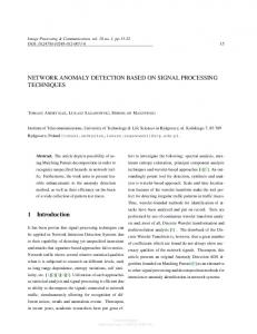
Effective Bot Host Detection Based on Network Failure Models Chun-Ying Huang Department of Computer Science and Engineering, National Taiwan Ocean University, 2 Pei-Ning Road, Keelung, Taiwan 20224
Abstract Botnet is one of the most notorious threats to Internet users. Attackers intrude into a large group of computers, install remote-controllable software, and then ask the compromised computers to launch large-scale Internet attacks, including sending spam and DDoS attacks. From the perspective of network administrators, it is important to identify bots in local networks. Bots residing in a local network could increase the difficulty to manage the network. Compared with bots outside of a local network, inside bots can easily bypass access controls applied to outsiders and access resources restricted to local users. In this paper, we propose an effective solution to detect bot hosts within a monitored local network. Based on our observations, a bot often has a differentiable failure pattern because of the botnet-distributed design and implementation. Hence, by monitoring failures generated by a single host for a short period, it is possible to determine whether the host is a bot or not by using a well-trained model. The proposed solution does not rely on aggregated network information, and therefore, works independent of network size. Our experiments show that the failure patterns among normal traffic, peer-to-peer traffic, and botnet traffic can be classified accurately. In addition to the ability to detect bot variants, the classification model can be retrained systematically to improve the detection ability for new bots. The evaluation results show that the proposed solution can detect bot hosts with more than 99% accuracy, whereas the false positive rate is lower than 0.5%. Key words: Botnet, network failure model, network management, network security
1. Introduction Botnet is one of the most notorious threat to Internet users. Based on the statistics provided by Kaspersky [1], more than 327 million attempts were made to infect users’ computers in different countries worldwide in the first quarter of 2010, which is 26.8% more than in the previous quarter. Botnet is a serious issue that security experts and researchers must investigate and solve.
Email address:
[email protected] (Chun-Ying Huang) Preprint submitted to Elsevier
August 15, 2012
Solutions to detect bot network activities can be classified into two approaches: misuse-based and anomaly-based. The misuse-based approach uses predefined patterns or signatures to compare against each network flow and identify malicious activities of a matching pattern. In contrast, the anomaly-based approach labels empirical network activities as normal or abnormal. Activities can then be further classified as normal or abnormal based on past observations. Although misuse-based approaches have benefits of enhanced performance and higher precision, they fail in detecting bot variants. A large database is often required to store the patterns and signatures used to detect bots. Therefore, developing anomaly-based detection techniques is a worthy endeavor. Numerous anomaly-based detection techniques already exist [2, 3, 4, 5, 6, 7, 8, 9, 10, 11, 12]. They detect bot activities based on features such as the amount, frequency, sequence, regularity, persistence, and similarity of network activities. However, these solutions have two common drawbacks. First, they must maintain numerous network flows for a period to extract features properly. Even with the traffic-filtering mechanism proposed in [11], approximately 30%1 of monitored traffic must be used for detection. Second, bot designers can easily evade some of these properties. One simple strategy is to add randomness to bot behavior. If well crafted, a bot can even behave like a human. Hence, we must still identify intrinsic and inevitable properties that cannot be evaded easily. An even more robust and systematic bot detection technique can be built on identified properties. Based on our understandings and observations of botnet traffic, it is intrinsic and inevitable for bots to generate network failures. Figure 1 shows two common scenarios of a bot generating failures. When a bot is awakened and joins a bot network, it must often find an entry point, either a command and control (C&C) server or a peer, to report its current status and obtain new commands. However, a C&C server is not always available because it could be shut down because of abuse reporting. The availability for peer-to-peer based botnets could worsen because peers can be shutdown or temporarily disconnected from the Internet at any instant. Therefore, attempting to establish communication channels with these computers could lead to failure, as shown in Figure 1(a). A new bot member may attempt several times to find an entry point. Alternatively, if it cannot find an entry point, it goes into a sleep state and attempts again after a period. Even if a bot successfully joins a bot network, it may follow the received commands to launch specific attacks. However, because most attacks are not limited to specific targets, it is also common for an attack to fail because the attacked target is temporarily unreachable, as shown in Figure 1(b). In this paper, we propose an anomaly-based bot host detection solution based on the network failure models. We collect network traces from both benign user computers and live bots, identify failures generated from each host, extract distinguishable features, and then build a classification model to classify benign hosts and bot hosts. To ensure that failures generated by distributed peer-to-peer hosts do not affect the accuracy of the classification model, we also classify peer-to-peer hosts. Our experiment results show that the proposed solution detects bot hosts with more than 99% accuracy, whereas the false positive and false negative rates are both lower than 0.5%. We also detect bots in real campus networks. Inspections show that 76 of 79 detected bot hosts in several 1 The
numbers are provided by the authors of the document.
2
(a) Join a botnet Bots
(b) Launch attacks
Off-line victims
Off-line C&C server
On-line victims
On-line C&C server
Figure 1: Origin of failures generated by bots.
Table 1: List of monitored failure types.
Protocol Type Description of the failure TCP i TCP SYN sent, but got TCP resets (RSTs) i TCP SYN send, but got ICMP unreachables t TCP SYN sent, but timed out UDP i UDP sent, but got ICMP unreachables t UDP sent, but timed out DNS i A DNS server responds errors to a queried domain
class-C networks are confirmed to be bots, whereas the remaining three hosts are highly suspected. The rest of this paper is organized as follows: Section 2 presents a detailed explanation of the proposed solution; Section 3 provides experimental results in both the laboratory and the field; Section 4 introduces several related works that inspired our research and a discussion on the limitations of this work; and finally, Section 5 offers a concluding remark. 2. The Proposed Solution Unlike numerous other bot detection algorithms, the proposed solution detects whether a host is a bot based only on information relevant to that host. It does not rely on aggregated network flows. Detection based only on single host information has two major benefits. First, the proposed solution works independent of the network size and is able to detect a bot host, despite only one compromised node residing in the monitored network. Second, detection time can be shortened. Because detection is made for each host, when the required number of feature samples collected from a single host is large enough, the decision can be made immediately. In the proposed solution, instead of counting the number of feature samples, we collect the required feature samples in a fixed period. 3
Training Phase Bot Traces
Peer-to-Peer Traces
Detection Phase Benign Traces
Real (or Test) Network Traces
Filter out non-failures (Traffic Reduction)
Filter out non-failures (Traffic Reduction)
Feature Extraction
Feature Extraction
Training (C4.5)
Classification
Model
Output Detection Result
Figure 2: The working flow of the detection system.
Hence, a compromised host can be detected within 2 to 3 minutes. The details of the proposed solution are introduced as follows. 2.1. Working Flow Figure 2 shows the working flow of the proposed solution. The flow can be divided into two parts: the training phase (left vertical path) and the detection phase (right vertical path). In the training phase, we collect numerous benign traces, peer-to-peer application traces, and bot traces, filter out non-failures, extract features from failure flows, and then build the classification model using the C4.5 [13] algorithm. In the detection phase, the process is similar to the training phase. Classification is made using the previously trained classification model. The performance of the proposed solution depends on both the representativeness of the training traces and the usefulness of the selected features. However, if the number of sampled traces and the number of selected features are large and diverse enough, the proposed solution would perform well. 2.2. Filter Out Non-Failures The proposed solution detects bots by inspecting failures generated by hosts. Therefore, non-failures should be filtered out because they are not used. A good strategy is to also reduce the system loads of memory storage and computation power. The number of failures is typically relatively smaller than successful cases on accessing benign network services. Filtering out non-failures greatly reduces the amount of network flows the system must process. Table 1 lists the types of failures that the proposed system monitors. For ease of explanation, we classify all failures into two types: immediate (type-i) and timed-out 4
Given an UDP packet
Inbound or Outbound?
PL: Pending List CL: Connected List
Inbound
Matched or Not Matched?
Not New
New Add a new 5-tuple into the PL
Matched
Not Matched
Outbound New or Not New
Update the timestamp of the 5-tuple if it is placed in the CL
Ignored
Move the 5-tuple from the PL to the CL
Figure 3: The state diagram used to maintain the connection state of each UDP flow.
(type-t) failures. True to its name, an immediate failure can be detected immediately after it occurs. In contrast, a timed-out failure can be detected after a period because no signal is delivered to notify senders. Whether a type-i or a type-t failure, a failure time stamp is always set to the time of the appearance of the first packet of a failed network flow. Type-i failures are easy to identify. However, some tricks are needed to identify type-t failures. For TCP, it is not difficult because a TCP flow must be established using the socalled three-way handshaking before any data are exchanged using the flow. Therefore, we only need to check the response to TCP SYN packets. If a TCP SYN packet is sent out, but there is no corresponding inbound TCP SYN-ACK packet, a corresponding inbound TCP RST packet, or a corresponding inbound ICMP unreachable packet received in a given period, we identify it as a TCP type-t failure. We use a threshold of 120 seconds to determine that a SYN packet has timed out because it is the default value used by the open-source Linux kernel’s connection tracking module. The case of UDP is relatively complex for two reasons. First, it is unnecessary for UDP flows to set up a connection before exchanging data. Second, UDP can be unidirectional, that is, packets can be sent in only one direction. To detect UDP type-t failures, we assume that most UDP-based application protocols are bidirectional. Hence, if only oneway traffic is observed within a given period, it could be an UDP type-t failure. The assumption is reasonable because in most cases, a sender has to ensure that a receiver has received what the sender sends so that additional data or messages can be sent. Based on this assumption, we maintain the “connection state” for each UDP flow using the procedures shown in Figure 3. The basic notion is to place failed UDP requests and successful UDP requests into the pending list (PL) and the connected list (CL), 5
An identified failure
Measurement time window
snapshot for failure #4
Current time T
snapshot for failure #12 time
1
2
3
4
5 67 8
9 10 11
snapshot for failure #8
12
13 14
15
snapshot for failure #15
Figure 4: Examples of snapshots for a single host. Snapshots are used to calculate feature vectors.
respectively. Suppose we are able to determine the direction of a UDP packet. For an outbound UDP packet, if the five-tuple2 is new to the system, it is added into the PL. A timestamp is also associated with the new five-tuple when it is added into the PL. The five-tuple is placed in the PL until the system receives a matched3 inbound UDP packet. On receipt of a matched inbound UDP packet, the corresponding five-tuple is moved from PL to CL. This also indicates that the previously sent UDP request did not fail because it is bidirectional. The timestamps of five-tuples placed in the CL are updated if data are exchanged using these flows. A connection remains active and prevents active five-tuples from being removed from the CL. If the timestamp of a five-tuple store in the PL or the CL has not been updated for a period, it is expired and removed from the lists. When a five-tuple is removed from the PL, a type-t failure is identified. In contrast, if a five-tuple is removed from the CL, it is treated as the termination of a normal UDP flow. Similar to the TCP case, we use 120 seconds as the threshold to determine whether a trial to establish an UDP connection is timed out. 2.3. Feature Extraction With the identified failures, numerous features are extracted from the observed failures on a per host basis. Before introducing how to extract features, we define the snapshot of failures (or simply snapshot) and the measurement time window (∆t). A snapshot is a list that contains a series of failures generated by a networked host. To limit snapshot length, at time T , only failures identified between T -∆t and T are included in the snapshot. A snapshot is taken when a failure is identified, as the example shown in Figure 4. Because 15 failures are identified in the figure, there should be 15 corresponding snapshots. However, to simplify the illustration, only four of them (snapshots for the 4th, 8th, 12th, and 15th failures) are shown in the figure. In the proposed solution, a snapshot is transformed into a feature vector. Numerous features (or attributes) are calculated based on failures within a snapshot and are listed in Table 2. The features are classified into the following six categories: 2 The five-tuple contains the source IP address, the destination IP address, the source port number, the destination port number, and the transport layer protocol. For ease of representation, we write a five-tuple in an abbreviated form of (source-IP, destination-IP, source-port, destination-port, protocol). 3 A “match” is defined as follows: With two packets p1 and p2 and their corresponding five-tuples t1 and t2, where t1 = (sip1, dip1, sport1, dport1, proto1) and t2 = (sip2, dip2, sport2, dport2, proto2). The two packets p1 and p2 are matched if and only if all the following conditions hold: 1) sip1=dip2; 2) dip1=sip2; 3) sport1=dport2; 4) dport1=sport2; and 5) proto1=proto2.
6
• Certain types of failures. • Average interval between failures. • Total number of failures. • Ratio of distinct destination port numbers. • Ratio of distinct destination IP addresses. • Average number of failures per destination IP address. We assume that feature vectors for normal, peer-to-peer, and bot hosts are differentiable. Hence, by collecting numerous feature vectors and assigning proper labels to feature vectors, these data can be used to train and build a classification model to differentiate normal, peer-to-peer, and bot hosts. In the training phase, the most important task is to assign proper labels to feature vectors. The proposed solution only has three labels: BOT, P2P, and NORM. To save human resources, we label feature vectors using the following strategies. For BOT, we first collect numerous live bots and then launch each bot on a clean virtual machine. The failures collected from virtual machines are used to build snapshots and are then transformed into feature vectors. All the output feature vectors are labeled as BOT. For P2P, similar to BOT, we also run peer-to-peer applications on clean virtual machines. The output feature vectors are then labeled P2P. NORM is slightly different because it is difficult to define what is normal and what is not. To obtain feature vectors capable to represent normal traffic, we assume that network traffic originated from certain computers in our laboratory as clean. All feature vectors calculated from failure snapshots of these computers are then labeled NORM. With feature vectors and labels, we feed these data to the C4.5 algorithm to build the final classification model. In the detection phase, with the same measurement time window, we take snapshots of failures from hosts residing in monitored networks. Feature vectors are then extracted from the snapshots. Each feature vector is classified as either NORM, P2P, or BOT by using the previously built classification model. Detecting whether a host is a bot is possible using “one-shot” classification; that is, classifying a host as a bot if and only if one feature vector is classified as BOT. However, in real-world cases, one-shot classification may lead to high false positive rates because of incomplete training data. In this case, it would be better if a decision can be made using majority votes to reduce possible high false positive rates. 3. Evaluation 3.1. Training Trace To evaluate the proposed solution, we first built a classification model from normal, peer-to-peer, and bot traces. The traces were collected in a controlled environment as described in Section 2.3. The normal traces were collected for five weekdays. We collected normal traces from four personal computers. All the personal computers were equipped with an Intel Core 2 Duo CPU and 2 GB of RAM. The installed operating system was Windows 7 Service Pack 1. We used tshark [14] to identify captured application 7
Table 2: List of features extracted from a snapshot of failures.
# 1 2 3 4 5 6 7 8 9 10 11 12 13 14 15 16 17 18 19 20 21 22 23 24
Data type real number real number real number real number real number real number real number real number boolean boolean boolean integer integer integer integer integer integer integer integer integer real number real number real number real number
25
real number
26
real number
27 28 29 30 31 32 33 34
real real real real real real real real
number number number number number number number number
Description Average interval between two adjacent TCP failures. Average interval between two adjacent TCP RESETs. Average interval between two adjacent TCP unreachable failures. Average interval between two adjacent TCP timeout failures. Average interval between two adjacent UDP failures. Average interval between two adjacent UDP unreachable failures. Average interval between two adjacent UDP timeout failures. Average interval between two adjacent DNS failures. Have TCP failures. Have UDP failures. Have DNS failures. Total number of TCP failures. Total number of TCP RESETs. Total number of TCP unreachable failures. Total number of TCP timeout failures. Total number of UDP failures. Total number of UDP unreachable failures. Total number of UDP timeout failures. Total number of DNS failures. Total number of all failures. Ratio of distinct destination ports to all destination ports. Ratio of distinct destination TCP ports to all destination TCP ports. Ratio of distinct destination UDP ports to all destination UDP ports. Ratio of distinct destination IP addresses to all destination IP addresses. (count all network flows) Ratio of distinct destination IP addresses to all destination IP addresses. (count only TCP network flows) Ratio of distinct destination IP addresses to all destination IP addresses. (count only UDP network flows) Average number of failures per destination IP addresses. Average number of TCP failures per destination IP addresses. Average number of TCP RESETs per destination IP addresses. Average number of TCP unreachable failures per destination IP addresses. Average number of TCP timeout failures per destination IP addresses. Average number of UDP failures per destination IP addresses. Average number of UDP timeout failures per destination IP addresses. Average number of DNS failures per destination IP addresses.
8
Table 3: Traffic profiles for the training traces. ID Norm #1 Norm #2 Norm #3 Norm #4 P2P #1 P2P #2 P2P #3 P2P #4 Bot #1 Bot #2 Bot #3 Bot #4 Bot #5 Bot #6 Bot #7
Total Volume 5,666 MB 6,317 MB 8,631 MB 9,163 MB 575 MB 146 MB 720 MB 422 MB 1,096 MB 78 MB 74 MB 19 MB 22 MB 89 MB 473 MB
Total Failures 8,829 347 1,408 588 5,700 5,716 20,623 303,983 5,135 215,224 5,403 21,582 6,440 3,761 10,440
RST 4,447 0 32 39 306 733 4,734 15,707 3 56,945 386 4,765 0 376 4,935
TCP Unreachable 4,292 0 62 0 0 0 455 253 0 0 0 0 0 0 519
Timeout 23 25 155 180 5,166 4,833 6,283 10,869 5,127 143,976 4,976 14,665 0 3,378 6
UDP Unreachable Timeout 16 10 153 134 22 614 26 173 10 217 1 149 693 8,443 11,619 265352 0 5 6,399 5 0 2 2,088 5 3,190 0 0 7 0 235
Table 4: The malware that generates traces.
# 1 2 3 4 5 6 7
MD5 783b28c65991292fdca1050cd4ae36ce e53d7aa295ce88aa456044343d5e0a66 9d2a48be1a553984a4fda1a88ed4f8ee 7d5e8af26f6acc81ab04a88f7f6ab459 fb367c916f23fd046c1c551a2280dfc4 70125984ed07048359f3bb4e44dc8c50 57864118b51d988938535293113e7a38
Name W32/Ircbot.1!Generic Trojan-Spy.Win32.Zbot.gen W32/SpyEyes.A.gen!Eldorado Trojan.Heur.Zbot.emW@c4@nf9c Backdoor.Bot.90879 W32/MalwareF.BOTJ W32/Mydoom.O@mm
protocols in the trace. The identified application protocols include DNS, FTP, HTTP, MSN, NFS, NTP, POP3, SMB, SMTP, SIP, SSH, SSL, and TELNET. The bot traces were also collected for five weekdays. We collected 30 malware samples from the Offensive Computing Web site [15]. Each malware is run on a virtual machine connected directly to the Internet. Among the 30 collected bot samples, only seven could be launched properly to generate network flows. Therefore, we show only the traces collected from these active bots. The seven bots are listed in Table 4. A malware can detect whether it is inside a virtual machine. If a virtual environment is detected, it does nothing to prevent it from being inspected. The method to collect peer-to-peer traces is the same as described in Section 2.3. However, each peer-to-peer client runs only for 12 hours for the following two reasons. First, unlike other applications, peer-to-peer clients are never idle and consistently attempt to complete download tasks. Therefore, it is possible to monitor and collect most behavior of peer-to-peer applications in a short time. Second, we were unable to run peer-to-peer clients in our campus network because of a global protocol filter for peer-topeer traffic installed in the campus. Running peer-to-peer clients in our campus would render us unable to monitor the peer-to-peer network traffic. Because of limited power and network access at home, we ran these peer-to-peer clients for a shorter period. We used the collected traces to build the detection model and cross-validate the model to show whether the solution works. Table 3 shows the trace profile for each collected trace. For a closer look at failure 9
DNS 41 35 523 170 1 0 15 183 0 7,899 39 149 3,250 0 4,745
40000
0
20000
40000
0
20000
0
40
80
(d) Normal #4 Number of Failures
40 20 0
5 10
Number of Failures
(c) Normal #3
40000
0
20000
40000
(e) Peer−to−Peer #1
(f) Peer−to−Peer #2
(g) Peer−to−Peer #3
(h) Peer−to−Peer #4
40000
0
20000
40000
0
20000
0
4000 1000
500 0 200
600 300
20000
4000
Time Offset (second)
Number of Failures
Time Offset (second)
Number of Failures
Time Offset (second)
Number of Failures
Time Offset (second)
0
40000
0
20000
40000
(i) Bot #1
(j) Bot #2
(k) Bot #3
(l) Bot #4
20000
40000
0
20000
40000
0
20000
40000
(m) Bot #5
(n) Bot #6
(o) Bot #7
20000
40000
Time Offset (second)
0
20000
40000
400 0
5 10
15 5 0
800
Time Offset (second)
Number of Failures
Time Offset (second)
Number of Failures
Time Offset (second)
0
Time Offset (second)
20000
40000
Time Offset (second)
Figure 5: Observed failures in the first 12 hours of each trace.
10
40 0
10 6 2
250 100
15 0
80
Time Offset (second)
Number of Failures
Time Offset (second)
Number of Failures
Time Offset (second)
Number of Failures
Time Offset (second)
5
Number of Failures
20000
0
Number of Failures
0
Number of Failures
(b) Normal #2 Number of Failures
25 15 5
Number of Failures
(a) Normal #1
0
20000
40000
Time Offset (second)
F21
8
F3
F30
BOT
P2P
F24
F13
NORM
BOT
P2P
8
F4
P2P
NORM
F16
NORM
P2P
F22
NORM
0.875
BOT
46.6391
NORM
F16
P2P
1
5
3.4475 F3
0.746
0.75
0.7889 0.5833 19.3602
P2P
NORM
BOT P2P
Figure 6: Decision tree generated from the training traces. The measurement time window (∆t) is set to 120 seconds.
patterns, we plot the amount of observed failures in the first 12 hours for each trace, as shown in Figure 5. The “Number of Failures” in the sub-figures of Figure 5 are cumulative failures in a 10-minute interval. From the figures, we can roughly observe that the failures for normal, peer-to-peer, and bot hosts are differentiable in amount and frequency. Figure 5 shows that normal clients generate only a limited number of failures (except for normal client #1, which is explained later). In contrast, peer-to-peer clients generate failures periodically and bots generate failures consistently or in a burst. Failures generated by peer-to-peer clients and bots appear diverse because these traces are generated by different peer-to-peer clients and bots. However, failures generated by normal client #1 are significantly different from those of other normal clients. We found that normal client #1 installed file-sharing client software [16] which is implemented as a Web-based peer-to-peer client. We did not remove failures generated by normal client #1 from this paper because the experiment results show that it does not affect the detection performance on bots. 3.2. Evaluation with Training Traces The benefit of evaluating with training traces is that we know the ground truth. Therefore, we can determine whether the selected features perform well on detection of normal, peer-to-peer, and bot hosts. We use K-fold cross-validation to verify the accuracy of the proposed solution. All of the labeled feature vector samples are partitioned into K groups randomly and the evaluation is run for K rounds. In each round, K-1 groups are selected as the training data and the remaining group is used to evaluate accuracy of the classifier. We choose K = 10 and conduct the experiments using the WEKA [17] machine-learning software. In each round, a new decision tree is generated using the C4.5 algorithm. The implementation of the C4.5 algorithm in the WEKA software is named J48. An example of the decision tree generated by the WEKA software is shown in Figure 6. The feature samples used to generate the decision tree are measured in a 120-second time window with 137 nodes in the tree. The maximum tree depth is 14 and the maximum tree width is 18. In the figure, intermediate nodes are marked in light gray. Leaf nodes, which are used to detect normal, peer-to-peer, and bot hosts, are marked in green, yellow, and 11
Peer−to−Peer vs Others
60
180
300
1200
3600
180
300
1200
3600
8e−04 6e−04 4e−04 2e−04 0e+00
60
Measurement Time Window (seconds)
Measurement Time Window (seconds)
FP Rate
0.9998 0.9996 0.9994 0.9992
Precision / Recall / F−Measure
10800 32400
Precision Recall (TP Rate) F−Measure FP Rate
0.9990
8e−04 6e−04
FP Rate
4e−04 2e−04 0e+00 60
10800 32400
1e−03
1.0000
Bot vs Others 1e−03
1.0000 0.9998 0.9996 0.9994 0.9992
Precision / Recall / F−Measure
Precision Recall (TP Rate) F−Measure FP Rate
0.9990
0.010 0.008 0.006 0.004 0.002 0.000
FP Rate
0.998 0.992
0.994
0.996
Precision Recall (TP Rate) F−Measure FP Rate
0.990
Precision / Recall / F−Measure
1.000
Normal vs Others
180
300
1200
3600
10800 32400
Measurement Time Window (seconds)
Figure 7: Summary of detection performance: Precision, recall, F-measure, and false positive rates.
red, respectively, to detect whether a feature sample is a normal, a peer-to-peer, or a bot host. The detection algorithm must walk an average of seven to eight steps in the decision tree before it is able to make a decision. 3.3. Detection Performance Figure 7 shows the precision, recall, F-measure, and false positive rates of all 10-fold cross-validation results. These numbers are obtained using the following equations. precision = recall =
true positives true positives + false positives
true positives true positives + false negatives
F-measure = 2 · FP rate =
precision · recall precision + recall
false positives true negatives + false positives
(1) (2) (3) (4)
Precision rates indicate the credibility of the reported detection result, whereas recall rates indicate the portion of hosts belonging to a specific class that can be identified. We use different scales of measurement time windows ranging from tens of seconds to half a day. The performance of each measurement time window is shown in Figure 7 in the order of 60, 120, 180, 240, 300, 600, 1200, 1800, 3600, 7200, 10800, 21600, 32400, and 43200 seconds. The results show that a larger measurement time window would result in enhanced detection performance in accuracy and false positive rate. Although we can use a large measurement time window such as half a day (43200 seconds), the response time to detect an unwanted event is also delayed. Based on the detection performance, to have a balance between the required detection time and the detection performance, a measurement time window between 180 seconds and 600 seconds would be a good choice. The detection accuracy shown in these figures is the “one-shot” classification performance, as explained at the end of Section 2.3. We also plot the receiver operating characteristic (ROC) curve for small measurement time windows. Discriminating whether a classifier performs well using ROC curve plots is common. Figure 8 shows ROC curve plots for measurement time windows of 60, 120, 12
Measurement Time Window = 120s
0.2
0.4
0.6
0.8
1.0 0.6 0.2 0.2
0.4
0.6
0.8
Normal vs Others Peer−to−Peer vs Others Bot vs Others
0.0
0.0
Normal vs Others Peer−to−Peer vs Others Bot vs Others
0.0
1.0
0.4
True Positive Rate
0.6 0.2
0.4
True Positive Rate
0.8
0.8
1.0 0.8 0.6 0.4
1.0
0.0
0.2
0.4
0.6
0.8
1.0
False Positive Rate
False Positive Rate
Measurement Time Window = 60s (Zoom−In)
Measurement Time Window = 120s (Zoom−In)
Measurement Time Window = 180s (Zoom−In)
0.2
0.4
0.6
0.8
1.0
1.000 0.4
0.6
0.8
0.998
0.999 0.2
0.997
True Positive Rate 0.0
0.995
0.996
0.998
Normal vs Others Peer−to−Peer vs Others Bot vs Others
0.994
Normal vs Others Peer−to−Peer vs Others Bot vs Others
0.994
0.994
Normal vs Others Peer−to−Peer vs Others Bot vs Others
0.0
0.997 0.995
0.995
0.996
0.997
True Positive Rate
0.998
0.999
0.999
1.000
1.000
False Positive Rate
0.996
True Positive Rate
0.2 0.0
Normal vs Others Peer−to−Peer vs Others Bot vs Others
0.0
True Positive Rate
Measurement Time Window = 180s
1.0
Measurement Time Window = 60s
1.0
0.0
0.2
False Positive Rate
False Positive Rate
0.4
0.6
0.8
1.0
False Positive Rate
Figure 8: ROC curves for small measurement time windows.
Table 5: Comparison of behavior-based botnet detection methods. Approach Core technique Bot samples Rate of traffic reduction True positive rate False positive rate
Livadas et al. [2] Machine learning 1 Re-implemented N/A 92% 11-15%
Gu et al. [5] Spatial-Temporal correlation 8 Mixed N/A 100% 0-6%
Wang et al. [11] Fuzzy-pattern 44 Real bots More than 70% 95% 0-3%
The proposed solution Machine learning 7/30 Real bots More than 75% 99% 0-0.2%
and 180 seconds. A perfect classifier would have an area under curve (AUC) of 1.0, but good classifiers would typically have a larger AUC close to 1.0 [18]. The figures show that the AUCs for the three small measurement time windows are all greater than 0.999. We conclude that the proposed solution performs well on classifying normal, peer-to-peer, and bot-hosts even when the measurement time window is small. 3.4. Performance Comparison Table 5 shows a comparison of several previous behavior-based botnet detection studies. The numbers for the previous studies are obtained from the corresponding papers. Therefore, the comparison of detection accuracies is evaluated independently by developers of each compared solution. Evaluation with different traces may lead to different results. However, we believe that evaluation with real traces would be better than with re-implemented and self-generated traces. The traffic reduction rate of the proposed solution is estimated by dividing the number of failed flows by the total number of flows. The actual traffic reduction rate is 76.04%, 13
but the traffic reduction rate can be substantially higher because bots and peer-to-peer clients contribute to most failures, and those hosts are rare in commercial and enterprise networks. If we inspect the traffic reduction rates for normal, peer-to-peer, and bot hosts independently, the traffic reduction rates are 99.08%, 42.40%, and 56.52%, respectively. The traffic reduction rate would be considerably enhanced in a real network because most clients in a monitored network are normal. The table also shows that the detection performance of the proposed solution is similar to and even better than previous research. In addition to good detection performance, the proposed solution requires only limited resources when online. The proposed solution detects bot hosts using a trained model. For the C4.5 algorithm, the model is the tree (as shown in Figure 6). If the model is stored using Weka’s default model file format, it costs only 30K bytes of storage. The computation costs required by the proposed solution are also limited. To detect bot hosts, the proposed solution must i) compute the features and ii) classify based on the trained model. For the first part, each monitored IP address requires only several counters to count the cumulative number of failures relevant to the monitored address in a time window. For the second part, the detection is made by traversing the tree model, which can be done in constant time. 3.5. Representativeness of Training Trace Choosing the traces to train the proposed solution is important. The representativeness of training traces affects detector performance greatly. To show how it affects detector performance, we conduct the following experiments to validate the assumption. We present 15 different traces collected from normal, peer-to-peer, and bot clients. For each experiment, we choose one trace as the test trace and the other 14 traces as the training traces. The model trained with the 14 training traces is then used to classify the test trace. Suppose a test trace is collected from a normal host. In a perfect classification, all the feature samples extracted from the test trace should be labeled NORM. However, if the test trace can be well classified, the representativeness of the test trace is low because it can be well classified, even if it is new to the classifier. If the test trace cannot be classified correctly, it can be used to represent and detect certain types of normal behavior. The heuristic applies to the other two types of traces, that is, P2P and BOT. Therefore, we are able to know the representativeness of training traces based on the test results. Table 6 shows the results of the experiments. Based on the results, we find that traces of normal client #4, peer-to-peer clients #1, #2, and #3, and bot client #1, #3, #4, and #6 have lower representativeness. This means that if we discard one of these traces, it would not affect detection performance significantly because the discarded parts can be complemented by other training traces. However, if a highly representative trace is discarded, for example, peer-to-peer client # 4 or bot client #7, we are unable to detect activities of that type of client. Therefore, it would be better to train the model using as many samples as possible to enhance detector capability. Table 6 also shows that the failure pattern of peer-to-peer clients is closer to normal clients and vice versa. If a highly representative bot is discarded, bot activity is often classified as NORM, and not P2P. 3.6. Detection in a Real Network We further implement the proposed solution in real networks. Hence, it is able to evaluate the performance of the proposed solution using real network traces on campus. 14
Table 6: Test the representativeness of training traces (window = 120s).
Excluded Training Trace Normal #1 Normal #2 Normal #3 Normal #4 P2P #1 P2P #2 P2P #3 P2P #4 BOT #1 BOT #2 BOT #3 BOT #4 BOT #5 BOT #6 BOT #7
Classified as NORM P2P 51.2% 45.2% 71.0% 29.0% 63.3% 32.8% 99.8% 0.1% 2.7% 97.1% 9.4% 88.1% 0.0% 100% 97.6% 2.4% 0.0% 0.0% 43.7% 0.2% 1.6% 0.0% 9.6% 0.1% 55.8% 0.0% 3.7% 0.0% 92.5% 0.0%
... BOT 3.6% 0.0% 3.9% 0.1% 0.2% 2.5% 0.0% 0.0% 100% 56.1% 98.4% 90.3% 44.2% 96.3% 7.5%
Campus Dormitory Network
Internet
Port Mirror
Detector
L3 Switch
Figure 9: The network setup to detect bots in real campus networks.
15
The network traces are collected on-the-fly using the libpcap [19] library. We implement traffic reduction and feature extraction in the C++ language. Model training and detection are conducted with the C4.5 release 8 [20] written by Ross Quinlan. We place the proposed solution at the edge of a campus dormitory network, as shown in Figure 9. Approximately 1000 hosts exist within the monitored network. The classification model is built using those traces collected in the controlled environment and we choose a short measurement time window of 120 seconds. Although we do not know whether bots reside in the monitored network, the proposed solution detects 79 suspected bots in the monitored network in 1 week. We verify whether an identified IP address is a bot by the following two steps: i) List all non-campus network IP addresses that have been contacted by an identified IP address; and ii) For each non-campus network IP address, look it up using search engines and check whether the address can be found in any blacklist. If an identified IP address has contacted a blacklisted peer, it could possibly be a bot. In addition to looking up addresses through search engines, we use publicly available blacklists such as [21] and [22] to shorten the required time to verify an address. Based on the heuristics, we found that 76 of the 79 identified IP addresses (96%) are confirmed to be bots. Although the remaining three IP addresses do not contact black-listed peers, they could possibly be bots because they have similar failure patterns to the trained malware. We do not investigate false negatives in the experiments of real network detections. This is because a blacklist only indicates an IP address or if a domain name behaves maliciously, but it does not tell us why it behaves maliciously. For example, the OpenBL blacklist [21] lists all hosts that have attempted to scan port 21 (ftp) and port 22 (ssh) services; the URLBlackList [22] categorizes malicious domain names into categories of malware, phishing, and spyware. Therefore, we are unable to distinguish whether a blacklisted address or site is used by a bot or other types of malicious behavior. However, a black-listed IP address indicates that the IP address of the owner’s machine has been compromised by attackers. That the machine has also been compromised by bot herders is highly possible. 4. Related Work Numerous studies have been devoted to botnet research. For ease of discussion, we classify bot detection mechanisms into two categories: group-based and individual-based solutions. Group-based solutions monitor activities from a group of hosts and make a decision based on aggregated information. In contrast, individual-based solutions detect bots based on observed events or activities from a single host. Several solutions detect botnets in a group-based manner. Choi et al. [3, 12] detected botnet activities by monitoring group activities in DNS traffic. Assume that a bot must look up the domain names of C&C servers. If a group of bots look up the domain names, the aggregated activities can be used to identify a group of bots. Gu et al. [5] detected botnet C&C channels by inspecting IRC and HTTP traffic. By capturing spatial-temporal correlation and using statistical algorithms, their system detected bot hosts within the same bot network. Another work by Gu et al. [6] involved detecting a botnet by clustering similar communication traffic and similar malicious communication traffic. They then performed cross-cluster correlation to identify hosts that share both similar communication traffic and similar malicious communication traffic. Consequently, if hosts within a group conduct similar 16
malicious activities and have similar communication patterns, they are detected as bots. One benefit of this work is that it does not need to know any bot beforehand. Several other solutions also detect bots in an individual manner. Most signature-based detection solutions such as Snort [23] can be classified as individual-based solutions. Gu et al. [4] proposed BotHunter to detect bots in a monitored network. They first defined the life-cycle of a bot. If the sequences of identified activities from a monitored host match parts of the life-cycle, it is identified as a bot. Giroire et al. [10] detected botnet C&C channels by observing connection persistence. This is because a bot must often obtain new instructions from a C&C server after a period. A host repeatedly contacting a remote host would have higher connection persistence. Based on this assumption, a bot can be detected by identifying hosts with higher connection persistence with littleknown remote hosts. Although well-known remote hosts such as Google or Yahoo would have higher persistence, with the help of white lists, the false positives can be reduced to a relatively low value. Gianvecchio et al. [7] detected IRC bots by inspecting the interval, length, frequency, and payload entropy of chat messages. Suppose the behavior of an IRC bot differs from that of a human. Their system collects identified network traffic characteristics and then distinguishes humans from bots using machine-learning techniques. Zhu et al. [24] proposed detecting bot activities based on application-level protocol failures. They collected application-level failures generated from DNS, HTTP, FTP, SMTP, and IRC traffic, measured the amount and frequency of failures, and then used machine-learning techniques to distinguish bots from benign hosts. Because the failures are collected at the application-level, they cannot handle encrypted traffic. Our proposed solution is classified as an individual-based solution and differs from previous research in several aspects. First, the proposed solution does not need to inspect payloads4 . Because payloads can be encrypted or obfuscated using standard techniques, reliance on payloads would limit detector ability. Second, we use intrinsic and inevitable network characters, that is, network failures. As described in Section 1, either joining a botnet or launching an attack would generate certain failures. Third, the detector does not need to analyze aggregated activities to make a decision. Even if only one compromised bot is residing in a monitored network, it can be identified. Finally, the proposed solution is able to detect bot hosts within several minutes, which is advantageous for a network administrator who wants to stop bots from ruining the network as soon as possible. Although the proposed solution performs well on detection of our available bots, there could be a malware that never generates failures. If such a malware exists, the proposed solution cannot detect it, even with captured traces generated from that malware. This type of malware should be treated as an advanced persistent threat (APT) and leave space for researchers to explore possible new detection techniques for APTs. 5. Conclusion Botnet is still a serious Internet issue. In this paper, we propose an effective solution that is able to detect bot hosts based on their network failure models. Bots generating 4 We only examine the payloads of DNS traffic delivered at UDP port 53. However, this is not a problem because even if DNSSEC is applied, DNS payloads are still readable because DNSSEC only authenticates a message instead of encrypting it.
17
network failures because of botnet-distributed design and implementation is intrinsic and inevitable. Evaluations show that the proposed solution achieves a high detection rate (more than 99%) and low false positive rates (less than 0.5%). Unlike previous anomalybased approaches, the proposed solution does not rely on aggregated group activities, does not need to examine payloads, and is able to detect bots in a short period. In addition to being efficient and robust, the proposed solution is lightweight in storage and computation costs. A portion of network traffic ranging from 42% to 99% can be filtered out to reduce system loads. Therefore, it can be deployed on either full-fledged personal computers or resource-constrained network devices to monitor different network scales. Acknowledgment This research was supported in part by National Science Council under the grants NSC 100-2221-E-019-045 and NSC 101-2219-E-019-001. We would like to thank the anonymous reviewers for their valuable and helpful comments. References [1] Kaspersky Security Bulletin, Information security threats in the first quarter of 2010, http://usa.kaspersky.com/resources/knowledge-center/information-security-threats-first-quarter2010 (May 2010). [2] C. Livadas, R. Walsh, D. Lapsley, W. T. Strayer, Usilng machine learning technliques to identify botnet traffic, in: Proceedings of the 31st IEEE Conference on Local Computer Networks, IEEE, 2006, pp. 967–974. [3] H. Choi, H. Lee, H. Lee, H. Kim, Botnet detection by monitoring group activities in dns traffic, in: Proceedings of the 7th IEEE International Conference on Computer and Information Technology, 2007. [4] G. Gu, P. Porras, V. Yegneswaran, M. Fong, W. Lee, Bothunter: Detecting malware infection through ids-driven dialog correlation, in: Proceedings of the 16th USENIX Security Symposium, 2007, pp. 167–182. [5] G. Gu, J. Zhang, W. Lee, Botsniffer: Detecting botnet command and control channels in network traffic, in: Proceedings of the 15th Network and Distributed System Security Symposium, 2008. [6] G. Gu, R. Perdisci, J. Zhang, W. Lee, Botminer: clustering analysis of network traffic for protocoland structure-independent botnet detection, in: Proceedings of the 17th USENIX Security Symposium, 2008. [7] S. Gianvecchio, M. Xie, Z. Wu, H. Wang, Measurement and classification of humans and bots in internet chat, in: Proceedings of the 17th conference on Security symposium, 2008. [8] J.-S. Lee, H. Jeong, J.-H. Park, M. Kim, B.-N. Noh, The activity analysis of malicious http-based botnets using degree of periodic repeatability, in: Proceedings of the International Conference on Security Technology, 2008. [9] G. Gu, V. Yegneswaran, P. Porras, J. Stoll, W. Lee, Active botnet probing to identify obscure command and control channels, in: Proceedings of Annual Computer Security Applications Conference, 2009, pp. 241–253. [10] F. Giroire, J. Chandrashekar, N. Taft, E. Schooler, D. Papagiannaki, Exploiting temporal persistence to detect covert botnet channels, in: Proceedings of the 12th International Symposium on Recent Advances in Intrusion Detection, 2009. [11] K. Wang, C.-Y. Huang, S.-J. Lin, Y.-D. Lin, A fuzzy pattern-based filtering algorithm for botnet detection, Computer Networks 55 (15) (2011) 3275–3286. [12] H. Choi, H. Lee, Identifying botnets by capturing group activities in dns traffic, Elsevier Computer Networks 56 (1) (2012) 20–33. [13] J. R. Quinlan, C4.5: programs for machine learning, Morgan Kaufmann Publishers Inc., 1993. [14] Wireshark Foundation, Wireshark—Go Deep, http://www.wireshark.org/.
18
[15] Offensive Computing, LLC., Offensive computing: Commnuity malicious code research and analysis, http://www.offensivecomputing.net/. [16] NEXTLiNK, Inc., GoGoBox, http://www.gogobox.com.tw/. [17] M. Hall, E. Frank, G. Holmes, B. Pfahringer, P. Reutemann, I. H. Witten, The WEKA data mining software: an update, SIGKDD Explorations Newsletter 11 (1) (2009) 10–18. [18] J. A. Hanley, B. J. McNeil, A method of comparing the areas under receiver operating characteristic curves derived from the same cases, Radiology 148 (3) (1983) 839–843. [19] Tcpdump/libpcap public repository, http://www.tcpdump.org/. [20] J. R. Quinlan, C4.5 release 8 source code, [on-line] http://www.rulequest.com/Personal/ (July 1999). [21] OpenBL.org, Blacklisting and abuse reporting, http://www.openbl.org/. [22] URLBlackList.com, URLBlackList.com, http://urlblacklist.com/. [23] M. Roesch, Snort - lightweight intrusion detection for networks, in: LISA’99: Proceedings of the 13th USENIX conference on system administration, 1999. [24] Z. Zhu, V. Yegneswaran, Y. Chen, Using failure information analysis to detect enterprise zombies, in: Security and Privacy In Communication Networks, 2009.
19