These schemes are designed for shock capturing and produce sharp ...... tions in a shock tube problem, the two-dimensional Euler equations in a forward.
MATHEMATICS OF COMPUTATION VOLUME 52, NUMBER 186 APRIL 1989, PAGES 509-537
Nonlinear Filters for Efficient Shock Computation By Björn Dedicated
Engquist,* to Professor
Per Lötstedt,** Eugene
Isaacson
and Björn
on the occasion
Sjögreen***
of his 70th
birthday
Abstract. A new type of methods for the numerical approximation of hyperbolic conservation laws with discontinuous solution is introduced. The methods are based on standard finite difference schemes. The difference solution is processed with a nonlinear conservation form filter at every time level to eliminate spurious oscillations near shocks. It is proved that the filter can control the total variation of the solution and also produce sharp discrete shocks. The method is simpler and faster than many other high resolution schemes for shock calculations. Numerical examples in one and two space dimensions are presented.
1. Introduction. A major difficulty in the numerical approximation of nonlinear hyperbolic conservation laws is the presence of discontinuities in the solution. Traditional schemes generate spurious oscillations in the numerical solution near these discontinuities. Standard methods based on centered differencing together with artificial viscosity have often during the last few years been replaced by the so-called high-resolution schemes. The high-resolution schemes are based on concepts like upwinding, local Riemann solvers, field by field decomposition and flux limiting, see, e.g., [1], [3], [12], [13]. These schemes are designed for shock capturing and produce sharp numerical discontinuities without oscillations. The algorithms are however not so computationally efficient. For higher-order numerical accuracy they are quite complicated.
It is our purpose to present a class of methods which retain most of the positive features of traditional schemes, but at the same time treat shocks and contacts similarly to the modern high-resolution schemes. The methods are based on standard schemes, the solutions of which are then processed with a nonlinear conservation law filter at every time step. The filter contains field by field decomposition and limiters in order to have good shock capturing properties. It is only activated at a few grid points, and therefore the overall algorithm has an order of accuracy and computational efficiency which are close to the traditional methods. The filter step is essentially independent from the step with the basic difference scheme. It is therefore easy to implement in existing codes. See the numerical examples in Section 6. Received January 18, 1988; revised June 20, 1988. 1980 Mathematics Subject Classification (1985 Revision). Primary 65M05, 65M10.
•Supported by NSF Grant No. DMS85-03294,NASA Consortium Agreement No. NCA2IR360-403. "Also at Aircraft Division, SAAB-SCANIA,S-581 88 Linköping, Sweden. "'Supported
by a grant from the Thanks to Scandinavia
Foundation ©1989
and by UCLA.
American
0025-5718/89
509 License or copyright restrictions may apply to redistribution; see http://www.ams.org/journal-terms-of-use
Mathematical
Society
$1.00 + $.25 per page
510
BJÖRN ENGQUIST, PER LOTSTEDT,
AND BJÖRN SJOGREEN
Our problem is a system of nonlinear hyperbolic conservation laws in, e.g., two space dimensions (ll)
\lt+f(u)X+g(u)y=0, u(x,y,0)
= u0(x,y),
with appropriate boundary conditions. The numerical Examples 3 and 4 in Section 6 are of this form. The method will first be described for the simpler one-dimensional case
(1.2)
»t + f(u)* = 0, u(i,0)
= u0(x),
when u and f are either scalars or vectors. We are interested in numerical approximations of weak solutions to (1.2) and assume that a consistent basic difference scheme of conservation form is already given, u]+1=G(u?_r,u?_r+1,...,u?+r),
(1.3)
u°j=u0(x),
n = 0,1,2,...,
j = ...,-1,0,1,...,
Xj ■=■ jAx, tn = nAt, Ai = AAx. We want to couple this scheme (in short form, un+1 = G(un)) projection in the following way:
with a filter or
vn+1=G(un), un+1 =P(vn+\un).
Let us here discuss some natural conditions for P. (1) Consistency. If the solution is smooth, the filter should not change the approximation vn+l too much. In particular, we want the total method (1.4) to be consistent, ||un+i _i/»+i|| =0(At2) for smooth vn+l.
The norm can, e.g., be the /i-norm, and smoothness may mean bounded higher divided differences. It is here possible to require that a higher order of accuracy of the basic scheme is not changed by the filter, see Subsection 2.2. (2) Conservation form. For convergence to the correct weak solution it is necessary for the total scheme (1.4) to be of conservation form, which means
(1.5)
5>(z,)«+1-^+1) |A_t>"+1|). (4) t>?+1 must not be decreased further than to the level of v"^_\, otherwise u"o+1 will pass the neighbor «?**, a case which we do not allow. The symbols A+ and A_ denote the forward and backward difference, respectively, A±u3 = ±(uj±i —Uj). These principles can be formulated in Algorithm 2.1 below. The vector u is to be understood as an array in a computer program, that initially contains the function to be filtered vn+1 and after completion of the algorithm
holds the filtered solution un+1.
Algorithm 2.1 for j := 2 to N - 1 do if (A+Uj)(A-u3) < 0 then if |A+Uj| > |A_Uj| then
6+ := |A+itj| 6- := |A_t»y| jcorr := j + 1 License or copyright restrictions may apply to redistribution; see http://www.ams.org/journal-terms-of-use
NONLINEAR FILTERS FOR EFFICIENT
SHOCK COMPUTATION
513
else
6+ := \A-Uj\ 6- := \A+Uj\ jcorr := j - 1
endif ¿:=min(¿_, TV(u") (Figure 2.3). This means that the method allows oscillations around the shocks, and indeed in numerical experiments there are oscillations present in the solution. These, however, have in most cases been observed to be of very small amplitude, cf. Table 6.1. (3) It flattens extrema that are not the result of overshooting and thus gives a low order of accuracy locally around smooth extrema, a property shared
with all TVD-schemes [6]. Algorithm 2.1 can be modified such that these difficulties are overcome. We continue by modifying Algorithm 2.1 to obtain a TVD-enforcing filter. As can be seen in Figure 2.3, v"+1 should sometimes decrease further. The question is how much. A stop condition is required. We have chosen to accept an extremum at jo if the condition (Cl)
min(uÂ-i>u"o>u"o+i)
^ 0 or d2 > 0) then correct Uj in the same way as in Algorithm 2.1, taking into account plateaus as described above, but with
6 :=min(6+/2,ö-,max(di,d2)) elseif (A+Uj)(A-Ui) < 0 and (A+wi_i)(A_up) < 0 then remove the zig-zagging as in Algorithm 2.2 with plateaus taken into account (p is the left index of the plateau that has
/ —1 as right index)
else comment:
if Uj does not need any correction go on to j + 1 newind(u, j + 1,1, j) endif endwhile The step that handles a consecutive maximum-minimum is not changed. This algorithm is optimal in the sense that it makes the smallest possible correction,
still being TVD. 2.2. Generalizations. The filters that were presented in Subsection 2.1 were either designed to produce TVD-solutions or they were simplifications of the TVDfilters. TVD-methods have a significant drawback. Enforcing a strict total variation
bound
EKii1-«r1iu in L\oc with u in L1 x L1 as Ax —► 0, Ai = XAx, then u is a weak solution to (1.2).
Proof. The proof is an extension of the convergence proof in [5] to include filter corrections. Let f(uR),
Xst
+ x,
UL > UR,
s = (f(uL) - f(uR))l(uL - uR). The case /(ul) < f(uR) is equivalent. Definition. A difference approximation to the above problem has a p-point discrete shock solution if there exists a solution of the form U" = UL,
UR < uu+r ^
= UR,
jjn+P,
License or copyright restrictions may apply to redistribution; see http://www.ams.org/journal-terms-of-use
526
BJÖRN ENGQUIST, PER LÖTSTEDT, AND BJÖRN SJÖGREEN
for all n. Let us introduce the notation Uj = V$,
Vj=v"+1,
Fíj = F(uí,Uj),
Fi = F(ui,Ui) = f(ui), where i and j may include L, R.
THEOREM5.1. The differencescheme (5.1) with the TVD-filter (Algorithm 2.3) has a solution with at most one point in the shock if ,co,
(5.3)
FL>F(u,uL),
uG(uR,uL),
FR>
uG(uR,uL),
F(uR,u),
and if the stepsizes satisfy a CFL-condition
(5.4)
A max
|/'(u)| < 1.
Ur uR.
(5.4), we have
uR < ui < uL. The filter step is executed and Uq+1 = vo, u™+1 = ii satisfy the original assumption. The case uo = uR is identical after an index shift. We thus need to analyze the
final situation uR UL, Vl < UR,
Vj = uR,
j > 1.
License or copyright restrictions may apply to redistribution; see http://www.ams.org/journal-terms-of-use
NONLINEAR FILTERS FOR EFFICIENT SHOCK COMPUTATION
527
Consider first vo > ul —(v~i —ui). The value at j = —1 will then be corrected as a plateau with vq until V-i =v0
= uL
if after conservative correction ñi < ul- The latter is true from total conservation
and (5.4), S_i +v0 + vi = i>_i + v0 + vi = uL + u0 + uR - X(FR - FL) < 3uL.
For vo < ul - (v-i -ul),v-i
will be corrected directly, resulting in
v-i =uL,
¿o = "o + (v-i - uL) < ul,
v0 = uo-
X(FR0 - Fol) - A(P0l - FL) = u0-
X(FR0 - FL).
From (5.2) and (5.3) we get vq > uq > uR. The final extremum is vi, which will be corrected to uR, changing vo to «"+1 = «o - X(FRo - FL) - X(FR - FRo) = u0- X(Fr - FL).
Thus, un+1 > tt0 > uR.
G
The condition (5.3) guarantees an oscillatory behavior at the left and right edges of the shock and a smoothing of the solution by the filter. In order to illustrate the result of this section, we choose the same formulation of the Lax-Wendroff scheme as in [3] and /¿ = /(tt¿). Then the numerical flux function is
f5 5)
Fi+Ui = \\fi + fi+i - {v2+i/2(ui+i - m)}, Vi+l/2 — ^at+l/2 = A5t)1+i = X(fi+i - fi)/(ui+i
- Ui).
The sufficient condition in Theorem 5.1 at the left edge for the scheme defined by
(5.5) is
FL - F(ui,uL) = \\2fL -fl-fi
+ A(/, - fL)2/(ut - uL)}
= \{Jl - A)[l - A(/i - h)/(ut - uL)}> 0. It follows from (5.6) that if /(wl) > f(ui) and (5.4) are satisfied for u¿ G (ur,ul), then the conditions for the state to the left of the shock is valid. The condition at the right edge for the scheme (5.5) is derived analogously.
The difference corresponding to (5.3) for Harten's TVD scheme [3] at a discrete
shock is
FL - F(u3,ul) = \{2fL -h= ±(uL
f} + {Ql, (u, - uL)\
- Uj)(XâLj -Qls),
where Q¿. is "the coefficient of numerical viscosity" [3], and j is the point in the
shock. In [3], Ql¡ is chosen such that Ql¡ > lAô^l when \Xa~L,\< 1. By (5.7) and the fact that u¿ > u, we have that Fl < FjL- There is no oscillation at the left edge, which is one purpose of the construction in [3], and no filtering is necessary. License or copyright restrictions may apply to redistribution; see http://www.ams.org/journal-terms-of-use
528
BJÖRN ENGQUIST, PER LOTSTEDT, AND BJÖRN SJÖGREEN
6. Numerical Results. The results of the numerical experiments with the filter and various difference schemes are presented. The conservation laws in our examples are the scalar inviscid Burgers' equation, the one-dimensional Euler equations in a shock tube problem, the two-dimensional Euler equations in a forward facing step problem and the two-dimensional steady Euler equations in the computation of flow around an airfoil. The first test problem is the inviscid Burgers' equation ut + (u2/2)x = 0,
«M) = {¿;
x 0.
TABLE 6.1 A propagating shock at t = 1.5; Burgers' equation. Lax-Wendroff+filter 2.1
2nd-order TVD scheme [3]
Lax-Wendroff+filter 2.4
81 82 83 84 85 86 87 88 89
1.000000004420621 1.000000004420621 0.9999993061366822 0.9999993061366822 1.000037711135951 1.015281066912056 1.015281066912056 0.2576304741863363 1.2105949518855330.E- 04
0.9999999999999990 0.9999999999998279 0.9999999999679732 0.9999999942705017 0.9999989269090302 0.9998095242194506 0.9670489441867344 0.3183558845540151 3.1261926819048629£
1.000000000000000 1.000000000000000 1.000000000000000 1.000000000000000 1.000000000000000 1.000000000000000 1.000000000000000 0.2882263480002554
90
2.7131497104461932E - 16
91
0.0OO0000O0000000OE + 00
1.0501687694116266E 3.1432670419155462E
03 05
1.2365199974462795Ê - 04 4.0132206279062878E - 16
08
0.0000000000000000£ + 00
This problem has been solved up to time = 1.5 with a CFL-number = 0.8. In the results in Table 6.1 the computed numbers are presented, because the difference between the results from different methods can be seen only in the second and
higher decimal places. For comparison, computations made with a 2nd-order TVD scheme (Harten [3]) are displayed. The filters 2.1 and 2.4 have been used together with the Lax-Wendroff scheme in [8]. This form of the Lax-Wendroff scheme is not the same as (5.5) at the end of Section 5, and (5.3) is not satisfied, but the schock is still fairly sharp. The results with and without filtering are illustrated in Figure 6.1.
The solution to Burgers' equation with a sine wave as initial condition, u(x,0) = 0.25+ 0.5 sin 7TX, was computed with the Lax-Wendroff scheme and the filter. At i = 0.75 a shock has developed, see Figure 6.2. In Table 6.2 the computed results in the neighborhood of the shock are displayed. The number of points in the shock is one also here. Theorem 5.1 seems to be valid even if the solution is not piecewise constant. License or copyright restrictions may apply to redistribution; see http://www.ams.org/journal-terms-of-use
NONLINEAR FILTERS FOR EFFICIENT SHOCK COMPUTATION
1.2
0. 8
0.6
H
0.4
i
0.2
H
0.0 ■1.0
-0. 5
0. 0
0. 5
1 .0
Figure 6.1 Shock solution for Burgers ' equation with the Lax- Wendroff scheme.
(a) without filter. (b) with the filter in Algorithm 2.4. License or copyright restrictions may apply to redistribution; see http://www.ams.org/journal-terms-of-use
529
530
BJÖRN ENGQUIST, PER LOTSTEDT, AND BJÖRN SJÖGREEN
The numerical solution is compared with the exact solution at t = 0.75. The numerical /i errors in the smooth part of the solution, i.e., at least a distance 0.1 away from the shock, are presented for three different spatial discretizations in Table 6.3. The results indicate that the smooth solution is second-order accurate.
Table 6.2 An initial sine wave has developed into a shock. Lax-Wendroff+filter 2.1
5 6 7 8 9 10 11 12 13 14
-
0.7510193076844476 0.7473223222626426 0.7333636414152179 0.7333636414152179 0.7333636414152179 0.4015613729134132 0.2195990067488021 0.2195990067488021 0.2354176977104853 0.2438072343976059
Figure 6.2 Shock solution at t = 0.75 for Burgers ' equation with the Lax- Wendroff scheme and filter and a sine wave as initial condition. License or copyright restrictions may apply to redistribution; see http://www.ams.org/journal-terms-of-use
NONLINEAR FILTERS FOR EFFICIENT SHOCK COMPUTATION
531
TABLE 6.3 The solutions to the sine wave problem have been processed
with filter 2.1 at each time level. Ax
0.005 0.01 0.02 0.04 0.005 0.01 0.02 0.04
Scheme
h error
Numerical order
LW
1.2 x 10⁻⁵ 4.4 X 10⁻⁵
1.9 2.0 2.4
LW LW LW Do Do Do Do
1.8 x 9.8 x 4.1 x 8.3 x 1.8 x 4.5 x
10-4 10~4 10-4 HT4 10-3 10-3
1.0 1.1 1.3
The TVD-filter enforces TVD independently of difference scheme and CFLnumber. It is possible to use large CFL-numbers and unstable schemes like u"+1 = un - AtDof(Uj) together with this filter, but the quality of the solution is of course affected negatively by large CFL-numbers. As an example, we have included results from using the filter together with the pure centered scheme above in Table 6.3. The obtained order of accuracy agrees with the expected one. In order to test the ability of Algorithm 4.1 to remove oscillations for systems of equations, we use the Euler equations and as initial data a function which consists of two constant states. This is a shock tube problem that has been used by many others as a test problem (e.g., [3], [11]). The equations are
pu p + pu2
u(e + p)
where p = (7 - l)(e - \pu2) and 7 = 1.4. The initial data are
x 0.
The solution consists of a shock followed by a contact discontinuity travelling to the right and a rarefaction wave going left. The solution at i = 2 is shown in Figure 6.3. There we used a CFL-number of 0.7. This problem could be run quite easily, but in problems containing very strong shocks there is a possibility that the difference scheme produces an overshooting point which is outside the region where c2 > 0. The square of the local sound speed c2 is computed as 7p/p. In order to correct such an overshoot, it is necessary to replace the decomposition into characteristic fields with an approximate one, which we have done in the two-dimensional computations below. License or copyright restrictions may apply to redistribution; see http://www.ams.org/journal-terms-of-use
532
BJÖRN ENGQUIST, PER LÖTSTEDT, AND BJÖRN SJÖGREEN
(a)
1.60 1.40 1.20
■
1.00
■
0.80 0.60
l_
0.40
■
0.20
■—i—' ~ ■"—i—"
0.00
50.
100.
200.
(b)
1.40
1.20
A
1.00
A
0.80 A
0.60 A 0.40
l_
A • l
50.
■ ■ ■ '
100.
l ■ ■ '
150.
'
i x
200.
Figure 6.3 Solution of a one-dimensional
shock tube problem with
the Lax- Wendroff scheme. (a) the density without filter. (b) the density with the filter in Algorithm 2.1. License or copyright restrictions may apply to redistribution; see http://www.ams.org/journal-terms-of-use
NONLINEAR FILTERS FOR EFFICIENT
SHOCK COMPUTATION
533
(b)
100.
150.
Figure 6.4 Solution of the forward facing step problem with the
Lax-Wendroffscheme and the 2D filter. (a) the density with 120 x 40 points. (b) the density with 240 x 80 points. We measured the CPU-time used to run this problem on a micro VAX, with the following result: TABLE 6.4 Method
CPU-seconds
Roe's method ULT1 Lax-Wendroff+Filter Lax-Wendroff
11 15 7 4
Roe's method is a first-order upwind scheme, described in [10], and ULT1 is a second-order TVD-scheme by Harten [3]. Let us also present some results from 2D-computations with the filter. The generalization to 2D is made by dimension splitting of the filter. That is, one time step is composed of the steps:
(a) Use a difference scheme to advance the solution to the next time level, not necessarily
by dimension
splitting.
(b) Apply the filter 4.1 in the x-direction. (c) Apply the filter 4.1 in the «/-direction. License or copyright restrictions may apply to redistribution; see http://www.ams.org/journal-terms-of-use
534
BJÖRN ENGQUIST, PER LÖTSTEDT,
0.00
0.00
0.50
0.50
1.00
1.00
1.50
1.50
Figure
AND BJÖRN SJÖGREEN
2.00
2.00
2.50
2.50
3.00
3.00
6.5
Solution of the forward facing step problem with the 4th-order centered difference scheme and the 2D filter.
(a) the density with 120 x 40 points. (b) the density with 240 x 80 points. We have here used the test problem "Mach-3 wind tunnel with a step" [13]. A gamma-law gas is fed in from the left into a channel of length 3 and width 1. The initial speed of the gas is Mach 3. At the lower side 0.6 from the right side of the channel, there is a step of height 0.2. The compressible Euler equations are solved for this problem, with 7 = 1.4. The solution is computed at i = 4, with a CFL-number of ¡=s 0.8. The step and the upper and lower walls of the channel are reflecting boundaries, with a Mach 3 uniform inflow on the left, and continuation boundary conditions on the right. In Figure 6.4 we show the solution computed with the dimension by dimension split Lax-Wendroff as the difference scheme. In Figure 6.5 we used a 4th-order centered difference scheme in space and 4th-order Runge-Kutta in time. The latter scheme gave initially an expansion shock emanating from the corner. In order to avoid this, we added a small amount of 4th-order dissipation to the scheme. The results presented in Figure 6.5 are computed with this dissipation added. Both these methods were unstable without
the filter. Finally, in order to illustrate the point that the filter can easily be implemented in an existing code, we have inserted it into a program that computes flow around an airfoil. The program was originally written by A. Rizzi and L.-E. Eriksson
License or copyright restrictions may apply to redistribution; see http://www.ams.org/journal-terms-of-use
NONLINEAR FILTERS FOR EFFICIENT SHOCK COMPUTATION
535
-cp
1.00
0.50 A 0.00 -0.50
-1.00 -1-'-'-1-■-1-■-1-•
0.00
0.20
x
0.40
0.60
0.80
1.00
-cp
1.00 A 0.50
0.00
-0.50
-1.00 —-1--"■-1-'-1-'-1-■-1-•
0.00
0.20
0.40
x
0.60
0.80
1.00
Figure 6.6 cp-plot of the Euler solution on the upper side of the airfoil. (a) with 2nd-order artificial viscosity according to [9]. (b) The 2nd-order artificial viscosity is replaced by the 2D filter.
[9] and uses 2nd-order centered difference approximation of the spatial derivatives with 2nd- and 4th-order artificial viscosity added. The 2nd-order dissipation term is introduced in order to damp oscillations at shocks. We removed the 2nd-order viscosity and inserted the filter. The time stepping is done with a Runge-Kutta type method. The grid used is of O-type and has 129 x 33 points. The freestream Mach number is 0.85 and the angle of attack Io. From this computation we present density contours and cp plots. Figures 6.6a and 6.7a show the density contours and Cpalong the upper surface of the airfoil computed by the original program. The 2ndorder artificial viscosity term is removed and the filter is introduced together with License or copyright restrictions may apply to redistribution; see http://www.ams.org/journal-terms-of-use
536
BJÖRN ENGQUIST, PER LÖTSTEDT, AND BJÖRN SJÖGREEN (a)
0.60-
0.40 -
0.20 -
0.00 --
-0.20
-
6
-0.40 -
-0 . 60 -I—,—,-1—|-,-1-,-,-1-1—,—,-1-1-1-1—,—.
0.00
(b)
0.50
x
1.00
V 0.60 -
0.40 -
0.20 -
0.00 -■
-0.20
-
-0.40
-
-0.60 0.00
0.50
1.00
1.50
Figure 6.7 Density contours for the same problem as in Figure 6.6. (a) with 2nd-order artificial viscosity according to [9]. (b) the 2nd-order artificial viscosity is replaced by the 2D filter. the 4th-order viscosity, giving the result in Figures 6.6b and 6.7b. This problem has weak shocks and the artificial viscosity method also computes a sufficiently good solution. The point we wanted to make here is the simplicity of introducing the filter into existing computer codes.
Department University
of Mathematics of California
at Los Angeles
Los Angeles, California 90024 License or copyright restrictions may apply to redistribution; see http://www.ams.org/journal-terms-of-use
NONLINEAR FILTERS FOR EFFICIENT SHOCK COMPUTATION
537
1. P. COLELLA, "Glimm's method for gas dynamics," SIAM J. Sei. Statist. Comput, v. 3, 1982, pp. 76-110. 2. D. GOTTLIEB, Spectral Methods for Compressible Flow Problems, Lecture Notes in Physics, No. 218 (Soubbaramayer and J. P. Boujot, eds.), Springer-Verlag, Berlin and New York, 1985, pp.
48-61. 3. A. HARTEN, "High resolution schemes for hyperbolic conservation
laws," J. Comput. Phys.,
v. 49, 1983, pp. 357-393. 4. A HARTEN & G. ZwAS, "Switched numerical Shuman filters for shock calculations,"
J.
Engrg. Math., v. 6, 1972, pp. 207-216. 5. P. LAX & B. WENDROFF, "Systems of conservation laws," Comm. Pure Appl. Math., v. 13,
1960, pp. 217-237. 6. S. OSHER & S. CHAKRAVARTHY, "High resolution schemes and the entropy condition,"
SIAM J. Numer. Anal., v. 21, 1984, pp. 955-984. 7. S. OSHER, A. HARTEN, B. ENGQUIST & S. CHAKRAVARTHY, "Some results on uniformly high-order accurate essentially nonoscillatory schemes," J. Appl. Numer. Math., v. 2, 1986, pp.
347-377. 8. R. D. RICHTMYER & K. W. MORTON, Differencemethodsfor Initial ValueProblems, 2nd ed., Interscience, New York, 1967. 9. A. RlZZI & L.-E. ERIKSSON, "Computation
of flow around wings based on the Euler
equations," J. Fluid Mech.,v. 148, 1984, p. 45-71. 10. P. L. ROE, "Approximate
Riemann solvers, parameter
vectors, and difference schemes," J.
Comput. Phys., v. 43, 1981, pp. 357-372. 11. G. A. SOD, " A survey of several finite difference methods for systems of nonlinear hyperbolic conservation laws," J. Comput. Phys., v. 27, 1978, pp. 1-31. 12. B. VAN LEER, "Towards the ultimate conservative difference scheme. V. A second-order sequel to Godunov's method," J. Comput. Phys., v. 32, 1979, 101-136. 13. P. R. WOODWARD & P. COLELLA, "The numerical simulation of two-dimensional fluid flow with strong shocks," J. Comput. Phys., v. 54, 1984, pp. 115-173.
License or copyright restrictions may apply to redistribution; see http://www.ams.org/journal-terms-of-use