based on the relative values of angles and some prede- fined thresholds. ... manually selected Triangular Fossa and Incisure Inter- tragica on the original 2D ...
Int Journal of Computer Vision manuscript No. (will be inserted by the editor) 1 Introduction
Efficient Detection and Recognition of 3D Ears Syed M. S. Islam, Rowan Davies, Mohmammed Bennamoun and Ajmal S. Mian
Received: 21 August 2009 / Accepted: 16 March 2011
Abstract The use of ear shape as a biometric trait is a recent trend in research. However, fast and accurate detection and recognition of the ear are very challenging because of its complex geometry. In this work, a very fast 2D AdaBoost detector is combined with fast 3D local feature matching and fine matching via an Iterative Closest Point (ICP) algorithm to obtain a complete, robust and fully automatic system with a good balance between speed and accuracy. Ear images are detected from 2D profile images using the proposed Cascaded AdaBoost detector. The corresponding 3D ear data is then extracted from the co-registered range image and represented with local 3D features. Unlike previous approaches, local features are used to construct a rejection classifier, to extract a minimal region with feature-rich data points and finally, to compute the initial transformation for matching with the ICP algorithm. The proposed system provides a detection rate of 99.9% and an identification rate of 95.4% on Collection F of the UND database. On a Core 2 Quad 9550, 2.83 GHz machine, it takes around 7.7 ms to detect an ear from a 640 × 480 image. Extracting features from an ear takes 22.2 sec and matching it with a gallery using only the local features takes 0.06 sec while using the full matching including ICP requires 2.28 sec on average. Keywords Biometrics, ear detection, 3D ear recognition, 3D local features, geometric consistency. School of Computer Science and Software Engineering, The University of Western Australia, 35, Stirling Highway, Crawley, WA 6009, Australia E-mail: {shams,rowan,m.bennamoun,ajmal}@csse.uwa.edu.au
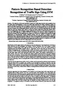
Instances of fraudulent breaches of traditional identity card based systems have motivated increased interest in strengthening security using biometrics for automatic recognition [31, 45]. Among the biometric traits, the face and the ear have received some significant attention due to the non-intrusiveness and the ease of data collection. Face recognition with neutral expressions has reached maturity with a high degree of accuracy [5, 28, 37, 58]. However, changes due to facial expressions, the use of cosmetics and eye glasses, the presence of facial hair including beard and aging significantly affect the performance of face recognition systems. The ear, compared to the face, is much smaller in size but has a rich structure [3] and a distinct shape [30] which remains unchanged from 8 to 70 years of age (as determined by Iannarelli [24] in a study of 10,000 ears). It is, therefore, a very suitable alternative or complement to the face for effective human recognition [6, 9, 23, 28]. However, reduced spatial resolution and uniform distribution of color sometimes makes it difficult to detect and recognize the ear from arbitrary profile or side face images. The presence of nearby hair and ear-rings also makes it very challenging for non-interactive biometric applications. In this work, we demonstrate that the Cascaded AdaBoost (Adaptive Boosting) [51] approach with appropriate Haar-features allows accurate and very fast detection of ears while being sufficient for a Local 3D Feature (L3DF) [37] based recognition. A detection rate of 99.9% is obtained on the UND Biometrics Database with 830 images of 415 subjects taking only 7.7 ms on the average using a C + + implementation on a Core 2 Quad 9550, 2.83 GHz PC. The approach is found to be significantly robust to ear-rings, hair and earphones. As illustrated in Fig. 1, the detected ear subwindow is cropped from the 2D and the corresponding co-registered 3D data and represented with Local 3D Features. These features are constructed by approximating surfaces around some distinctive keypoints based on the neighboring information. When matching a probe with a gallery, a rejection classifier is built based on the distance and geometric consistency among the feature vectors. A minimal rectangular region containing all the matching features is extracted from the probe and the best few gallery candidates. These selected and minimal gallery-probe datasets are coarsely aligned based on the geometric information extracted from the feature correspondences and then finely matched via the Iterative Closest Point (ICP) algorithm. While evaluating the performance of the complete system on the
2
Ear Detection and Ear Data Extraction
Ear Data Normalization
Keypoint Identification
3D Local Features Extraction
On-line probe features L3DF-based Matching 2D and 3D Profile Face Data Recognition Decision
Fine Matching with ICP
Off-line storage of gallery features
Gallery Features
Coarse Alignment Using Feature Correspondences
Recognized Ear
Fig. 1 Block diagram of the proposed ear detection and recognition system.
UND-J, the largest available ear database, we obtain an identification rate of 93.5% with an Equal Error Rate (EER) of 4.1%. The corresponding rates for the UND-F dataset are 95.4% and 2.3% and the rates for a new dataset of 50 subjects all wearing ear-phones are 98% and 1%. With an unoptimized MATLAB implementation, the average time required for the feature extraction, the L3DF-based matching and for the full matching including ICP are 22.2, 0.06 and 2.28 seconds respectively. The rest of the paper is organized as follows. Related work and contributions of this paper are described in Section 2. The proposed ear detection approach is elaborated in Section 3. The recognition approach with local 3D features is explained in Sections 4 and 5. The performance of the approaches are evaluated in Sections 6 and 7. The proposed approaches are compared with other approaches in Section 8 followed by a conclusion in Section 9. 2 Related Work and Contributions In this section, we describe the methodology and performance of the existing 2D and 3D ear detection and recognition approaches. We then discuss the motivation inspired from the limitations of these approaches and highlight the contributions of this paper. 2.1 Ear Detection Approaches Based on the type of data used, existing ear detection or ear region extraction approaches can be classified
as 2D, 3D and multimodal 2D+3D. However, most approaches use only 2D profile images. One of the earliest 2D ear detection approaches is proposed by Burge and Burger [6] who used Canny edge maps [8] to find the ear contours. Ansari and Gupta [2] also used a Canny edge detector to extract the ear edges and segmented them into convex and concave curves. After the elimination of non-ear edges, they found the final outer helix curve based on the relative values of angles and some predefined thresholds. They then joined the two end points of the helix curve with straight lines to get the complete ear boundary. They obtained 93.3% accuracy of localizing the ears on a database of 700 samples. Ear contours were also detected based on illumination changes within a chosen window by Chora´ s [15]. The author compared the difference between the maximum and minimum intensity values of a window to a threshold computed from the mean and standard deviation of that region in order to decide whether the center of the region belongs to the contour of the ear or to the background. Ear detection approaches that utilize 2D template matching include the work of Yuizono et al. [56] where both hierarchical and sequential similarity detection algorithms were used to detect the ear from 2D intensity images. Another technique based on a modified snake algorithm and an ovoid model was proposed by Alvarez et al. [1]. It requires the user to input an approximated ear contour which is then used for estimating the ovoid model parameters for matching. Yan and Bowyer [54] manually selected Triangular Fossa and Incisure Intertragica on the original 2D profile image and drew a line to be used as a landmark. One line was along the border between the ear and the face, and the other from
3
the top of the ear to the bottom. The authors found this method suitable for PCA-based and edge-based matching. The Hough Transform can extract shapes with properties equivalent to template matching and was used by Arbab-Zavar and Nixon [3] to detect the elliptical shape of the ear. The authors successfully detected the ear region in all of the 252 profile images of a non-occluded subset of the XM 2V T S database. For the UND database, they first detected the face region using skin detection and the Canny edge operator followed by the extraction of the ear region using their proposed method with a success rate of 91%. They also introduced synthetic occlusions vertically from top to bottom on the ear region of the first dataset and obtained around 93% and 90% detection rates for 20% and 30% occlusion respectively. Recently, Gentile et al. [19] used AdaBoost [51] to detect the ear from a profile face as part of their multi-biometric approach for detecting drivers’ profiles in a security checkpoint. In an experiment with 46 images from 23 subjects, they obtained an ear detection rate of 97% with seven false positives per image. They did not report the efficiency of their system. Approaches using only 3D or range data include Yan and Bowyer’s two-line based landmarks and 3D masks [54], Chen and Bhanu’s 3D template matching [10] and the ear-shape-model based approach [12]. Similar to their 2D technique [54] mentioned above, Yan and Bowyer [54] drew two lines on the original range image to find the orientation and scaling of the ear. They rotated and scaled a mask accordingly and applied it on the original image to crop the 3D ear data in an ICP-based matching approach. Chen and Bhanu [10] combined template matching with average histogram to detect ears. They achieved a 91.5% detection rate with about 3% False Positive Rate (FPR). In [12], they represented an ear shape model by a set of discrete 3D vertices on the ear helix and anti-helix parts and aligned the model with the range images to detect the ear parts. With this approach, they obtained 92.5% detection accuracy on the University of California, Riverside (UCR) ear dataset with 312 images and an average detection time of 6.5 sec on a 2.4 GHz Celeron CPU. Among the multimodal 2D+3D approaches, Yan and Bowyer [55] and Chen and Bhanu [13] are prominent. In the first approach, the ear region was initially located by taking a predefined sector from the nose tip. The non-ear portion was then cropped out from that sector using a skin detection algorithm and the ear pit was detected using Gaussian smoothing and curvature estimation algorithms. An active contour algorithm was applied to extract the ear contour. Using the color and the depth information separately for the active contour, ear
detection accuracies of 79% and 85% respectively were obtained. However, using both 2D and 3D information, ears from all the profile images were successfully extracted. Thus, the system is automatic but depends highly on the accuracy of detection of nose tip and ear pit and it fails when the ear pit is not visible. Chen and Bhanu [13] also used both color and range images to extract ear data. They used a reference ear shape model based on the helix and anti-helix curves and the global-to-local shape registration. They obtained 99.3% and 87.7% detection rates while tested on the UCR ear database of 902 images from 155 subjects and on 700 images of the UND database, respectively. The detection time for the UCR database is reported as 9.5 sec with a MATLAB implementation on a 2.4 GHz Celeron CPU. 2.2 Ear Recognition Approaches Most of the existing ear recognition techniques are based on 2D data and extensive surveys can be found in [28, 44]. Some of them report very high accuracies but on smaller databases; e.g. Chora´ s [15] obtained 100% recognition on a database of 12 subjects and Hurley et al. [22] obtained 99.2% accuracy on a database of 63 subjects. As expected, performance generally drops for larger databases, e.g. Yan and Bowyer [53] report a performance drop from 92% to 84.1% for database sizes of 25 and 302 subjects respectively. Also, most of the approaches do not consider occlusion in the ear images (e.g. [21, 35, 11, 22, 57, 16]). Considering these issues and the scope of the paper, only those approaches using large 3D databases and somewhat occluded data are summarized in Table 1 and described below. Yan and Bowyer [55] applied 3D ICP with an initial translation using the ear pit location computed during the ear detection process. They achieved 97.8% rank-1 recognition with an Equal-error rate (EER) of 1.2% on the whole UND Collection J dataset consisting of 1386 probes of 415 subjects and 415 gallery images. They obtained a recognition rate of 95.7% on a subset of 70 images from this dataset which have limited occlusions with earrings and hair. In another experiment with the UND Collection G dataset of 24 subjects each having a straight-on and a 45 degrees off center image, they achieved 70.8% recognition rate. However, the system is not expected to work properly if the nose tip or the ear pit are not clearly visible which may happen sometimes due to pose variations or covering with hair or ear-phones (see Fig. 10 and 12). Chen and Bhanu [13] used a modified version of ICP for 3D ear recognition. They obtained 96.4% recognition on Collection F of the UND database (including
4 Table 1 Summary of the existing 3D ear recognition approaches Publication
Methodology Dataset
Name
Yan and Bowyer, 2007 [55] Chen and Bhanu, 2007 [13]
Passalis et al., 2007 [43] Cadavid and AbdelMottaleb, 2007 [7] Yan and Bowyer, 2005 [53]
3D ICP LSP and 3D ICP
UND-J
Rec. Rate (%) Size (gallery, probe) (415, 97.8 1386)
UCR
(155, 155)
96.8
UND-F
(302, 302) (415, 415)
96.4
AEM, ICP, DMF
UND-J
3D ICP
Proprietary
(61, 25)
84
UND-F
(302, 302)
84.1
3D ICP
ing left and right ears seems relatively easy. In cases where both profile images are not available, extracted ear data from the opposite profile can be mirrored for matching with still relatively reliable recognition. Yan and Bowyer [54, 55] experimentally demonstrated that although some people’s left and right ears have recognizably different shapes, most people’s two ears are approximately bilaterally symmetric. They obtained around 90% recognition rate while matching mirrored left ears to right ears on a dataset of 119 subjects. We have focused on left ears, but the above work suggests our research can be used in other situations also.
93.9
occluded and non-occluded images of 302 subjects) and 87.5% recognition for straight-on to 45 degree off images. They obtained 94.4% rank-1 recognition rate for the UCR dataset ES2 which comprises 902 images of 155 subjects taken all in the same day. They used local features for representation and coarse alignment of ear data and obtained a better performance than their helix-anti-helix representation. Their approach assumes perfect ear detection, otherwise manual extraction of the ear contour is performed prior to recognition. Passalis et al. [43] used a generic annotated ear model (AEM), ICP and Simulated Annealing algorithms to register and fit each ear dataset. They then extracted a compact biometric signature for matching. Their approach required 30 sec for enrolment per individual and less than 1 ms for matching two biometric signatures on a Pentium 4, 3 GHz CPU. They computed the full similarity matrix with 415 columns (galleries) and 415 rows (probes) for the UND-J dataset taking seven hours of enrolment and few minutes of matching and achieved 93.9% recognition rates. Cadavid and Abdel-Mottaleb [7] extracted a 3D ear model from video sequences and used 3D ICP for matching. They obtained 84% rank one recognition while testing with a database of 61 gallery and 25 probe nonoccluded images. All of the above recognition approaches have only considered left or right ears. An exception is Chora´ s [16] who proposed to pre-classify each detected ear as left or right based on the geometrical parameters of the earlobe. The author reported accurate pre-classification of all 800 images from 80 subjects. Hence, distinguish-
2.3 Motivations and Contributions Most of the ear detection approaches mentioned above are not fast enough to be applied in real-time applications. Viola and Jones have used the AdaBoost algorithm [18, 46] to detect faces and obtained a speed of 15 frames per second while scanning 384 by 288 pixel images on a 700 MHz Intel Pentium III [51]. For this extreme speed and simplicity of implementation, AdaBoost has further been used for detecting the ball in a soccer game [47], pedestrians [40], eyes [42], mouths [34] and hands [14]. However, existing ear detection using AdaBoost (see Section 2.1) does not achieve significant accuracy. In fact, even for faces, Viola and Jones [51] obtained only 93.7% detection rate with 422 false positives on MIT+CMU face database. Ear detection is more challenging because ears are much smaller than faces and often covered by hair, ear-rings, ear-phones etc. Challenges lie in reducing incorrect or partial localization while maintaining high correct detection rate. Hence, we are motivated to determine the right way to instantiate the general AdaBoost approach with the specifics required in order to specialize it for ear detection. Most of the ear recognition approaches use global features and ICP for matching. Compared to local features, global features are more sensitive to occlusions and variations in pose, scale and illumination. Although ICP is considered to be the most accurate matching algorithm, it is computationally expensive and it requires concisely cropped ear data and a good initial alignment between the galley-probe pair so that it does not converge to a local minimum. Yan and Bowyer [55] suggested that the performance of ICP might be enhanced using feature classifiers. Recently, Mian et al. [37] proposed local 3D features for face recognition. Using these features alone, they reported 99% recognition accuracy on neutral versus neutral and 93.5% on neutral versus all on the FRGC v2 3D face dataset. They also obtained a time efficiency of 23 matches per second on a 3.2 GHz
5
Pentium IV machine with 1GB RAM. In this paper, we adapt these features for the ear and use them for coarse alignment as well as for rejecting a large number of false matches. We also use L3DFs for extracting a minimal set of datapoints to be used in ICP. The specific contributions of this paper are as follows: (1) A fast and fully automatic ear detection approach using cascaded AdaBoost classifiers trained with three new features and a rectangular detection window. No assumption is made about the localization of the nose or the ear pit. (2) The local 3D features are used for ear recognition in a more accurate way than originally proposed in [37] for the face including an explicit second round of matching based on geometric consistency. L3DFs are used not only for coarse alignment but also for rejecting most false matches. (3) A novel approach for extracting minimal featurerich data points for the final ICP alignment is proposed which significantly increases the time efficiency of the recognition system. (4) Experiments are performed on a new database of profile images with ear-phones along with the largest publicly available dataset of the UND and high recognition rates are achieved without an explicit extraction of the ear contours.
3 Automatic Detection and Extraction of Ear Data The ear region is detected on 2D profile images using a detector based on the AdaBoost algorithm [18, 46, 26, 27]. Following [51], Haar-like features are used as weak classifiers and learned from a number of ear and non-ear images. After training, the detector first scans through the 2D profile images to identify a small rectangular region containing the ear. The corresponding 3D data is then extracted from the co-registered 3D profile data. The complete detection framework is shown in the block diagram of Fig. 2. A sample of a profile image and the corresponding 2D and 3D ear data detected by our system is also shown in the same figure. The details of the construction of the detector and its functional procedures are described in this section.
3.1 Feature Space The eight different types of rectangular Haar feature templates as shown in Fig. 3 are used to construct our AdaBoost based detector. Among these, the first five
Collect 2D and 2D 3D Profile Face Data
Preprocess 2D Data
Validate and Update with False Positives
Create Rectangular Haar Features
Train Classifiers Using Cascaded AdaBoost
2D Profile
3D Profile
Scan and Detect 2D Ear Region
Off-line Training On-line Detection
Extracted 2D Ear
Extract 3D Ear Data Extracted 3D Ear
Fig. 2 Block diagram of the proposed ear detection approach.
(a-e) were also used by Viola and Jones [51] to detect different types of lines and curves in the face. We devised the later three templates (f-h) to detect specific features of the ear which are not available in the frontal face. The center-surround template is designed to detect any cavity in the ear (e.g. ear pit) and the other two (adopted from [32]) are for detecting helix and the anti-helix curves. Although (f) is the intersection of (c) and (e), we use it as a separate feature template because no linear combination of those features yields (f) and as will be discussed in the next sub-section, the AdaBoost algorithm used for feature selection greedily chooses the best individual Haar features, rather than their best combination.
(a)
(b)
(c)
(d)
(f)
(g)
(h)
(e)
Fig. 3 Features used in training the AdaBoost (features (f), (g) and (h) are proposed for detecting specific features of the ear) .
To create a number of Haar features out of the above eight types of templates or filters, we choose a window to which all the input samples are normalized. Viola and Jones [51] used a square window of size 24 × 24 for face detection. Our experiments with training data show that ears are roughly proportional to a rectan-
6
gular window of size 16 × 24. One benefit of choosing a smaller window size is the reduction of training time and resources. The templates are shifted and scaled horizontally and vertically along the chosen window and a feature is numbered for each location, scale and type. Thus, for the chosen window size and a shift of one pixel, we obtain an over-complete basis of 96413 potential features. The value of a feature is computed by subtracting the sum of the pixels in the grey region(s) from that of the dark region(s) (except in the case of (c), (e) and (f) in Fig. 3, where the sum in the dark region is multiplied by 2, 2 and 8 respectively before performing the subtraction in order to make the weight of this region equal to that of the grey region(s)).
3.2 Construction of the Classifiers The rectangular Haar-like features described above constitute the weak classifiers of our detection algorithm. A set of such classifiers are selected and then combined together to construct a strong classifier via AdaBoost [18, 46] and a sequence of these are then cascaded following Viola and Jones [51]. Thus, each strong classifier in the cascade is a linear combination of the best weak classifiers, with weights inversely proportional to training errors on those examples not previously rejected by an early stage of the cascade. This results in a fast detection as most of the negative sub-windows are rejected using only a small number of features associated with the initial stages. The optimization of the number of stages, the number of features per stage and the threshold for each stage for a target detection rate (D) and false positive rate (Ft ) is obtained similar to [51] by aiming for a fixed maximum FPR (fm ) and a minimum detection rate (dmin ) for each stage. These are computed from the following inequalities: Ft < (fm )n and D > (dmin )n , where n is the number of stages, typically 10-50.
3.3 Training the Classifiers The training dataset to build the proposed ear detector, their preprocessing stage, the training parameters chosen and other implementation aspects are described as follows. 3.3.1 Dataset The positive training set is built with 5000 left ear images cropped from the profile face images of different
databases covering a wide range of races, sexes, appearances, orientations and illuminations. This set includes 429 images of the University of Notre Dame (UND) Biometrics Database (Collection F) [49, 55], 659 of the NIST Mugshot Identification Database (MID) [41], 573 of XM2VTSDB [36], 201 images of the USTB [50], 15 of the MIT-CBCL [52, 39], and 188 of the UMIST [20, 48] face databases. It also includes around 3000 images synthesized by rotating -15 to +15 degrees of some images from the USTB, the UND and the XM2VTSDB databases. Our negative training set for the first stage of the cascade includes 10,000 images randomly chosen from a set of around 65,000 non-ear images. These images are mostly cropped from profile images excluding the ear area. We also include some images of trees, birds and landscapes randomly downloaded from the web. Examples of the positive and negative image set are shown in Fig. 4. The negative training set for the second and subsequent stages are made up dynamically as follows. A set of 6000 large images without ears are scanned through at the end of each stage of the cascade by the classifier developed in that stage. Any sub-window classified as an ear is considered as a false positive and a set of not more than 5000 such false positives are randomly chosen to include in the negative set for the following stages.
Fig. 4 Examples of ear (top) and non-ear (bottom) images used in the training.
The validation set used to compute the rates of detection and false positives during the training process includes 5000 positives (cropped and synthesized ear images) and 6000 negatives (non-ear images). The negatives for the first stage are randomly chosen from a set of 12000 images not included in the training set. For the second and the subsequent stages, negatives are randomly chosen from the false positives found by the classifier of the previous stage and unused in the negative training set. 3.3.2 Preprocessing the Data As mentioned earlier, input images are collected from different sources with varying size and intensity values. Therefore, all the input images are scale normalized to the chosen input pattern size. Viola and Jones
7
reported a square input pattern of size 24 × 24 as the most suitable for detecting frontal faces [51]. Considering the shape of the ear, we instead use a rectangular pattern of size 16 × 24. The variance of the intensity values of images are also normalized to minimize the effect of lighting. Similar normalization is performed for each sub-window scanned during testing. 3.3.3 Training the Cascade In order to train the cascade, we choose Ft = 0.001 and D = 0.98. However, to quickly reject most of the false positives using a small number of features, we define the first four stages to be completed with 10, 20, 60 and 80 features. We also performed validation after adding ten features for the first ten stages and then, adding of 25 for the remaining stages. The detection and false positive rates computed during the validation of each stage follow a gradual decrease to the target. The training finishes at stage 18 with a total of 5035 rectangular features including 1425 features in the last stage.
and Jones [51] who also illustrated this to be more timeefficient than the conventional pyramid approach. If the rectangular detector (of 16×24 or its scaled-up size) matches any sub-window of the image, a rectangle is drawn to show the detection (See Fig. 5). The integration of multiple detections (if any) is described in the following sub-section and the overall performance of the detector is discussed in Section 6. As mentioned in Section 3.3, our system is trained for detecting ears from the left profile images only. However, if the input image is a right profile and the ear detector fails, then the features constituting the detector can be flipped to detect the right ears.
3.3.4 Training Time The training process involved a huge amount of computation due to the large training set and also for the very low target FPR, taking several weeks on a single PC. To speed up the process, we distributed the job over a network of around 30 PCs. For this purpose, we used M AT LABM P I which is a MATLAB implementation of the Message Passing Interface (MPI) standard that allows any MATLAB program to exploit multiple processors [33]. It helped in reducing the training time to an order of days. An optimized C or C + + implementation would reduce this time, but since this training never needs to be done again, our MATLAB implementation was sufficient. 3.4 Ear Detection with the Cascaded Classifiers The trained classifiers of all the stages are used to build the ear detector in a cascaded manner. The detector is scanned over a test profile image in different sizes and locations. A classifier in the cascade is only used when a sub-window in the test image is detected as positive (ear) by the classifier of the previous stage and accepted finally only when it passes through all of them. To detect various sizes of ears, instead of resizing the given test image, we scale up the detector along with the corresponding features and use an integral image calculation. The approach is similar to that of Viola
Fig. 5 Sample of detections: (a) Detection with single window. (b) Multi-detection integration (Color online).
3.5 Multi-detection Integration Since the detector scans over a region in the test image with different scales and shift sizes, there is the possibility of multiple detections of the ear or ear-like regions. To integrate such multiple detections, we propose the clustering algorithm reported in Algorithm 1. The clustering algorithm is based on the percentage of overlap of the rectangles representing the detected sub-windows. We cluster a pair of rectangles together if the mutual area shared between them is larger than a predefined threshold, minOv (0 < minOv < 1). A higher value of this parameter may result in multiple detections near the ear. We empirically chose a threshold value of 0.01. Based on the observation that the number of true detections at different scales over the ear region is larger than the false detections on ear-like region(s) (if any), we added an option in the algorithm to avoid such false positive(s) by only taking the one that clusters the maximum number of rectangles. This is appropriate when
8
only one ear needs to be detected which is the case for most recognition applications.
3.7 Extracted Ear Data Normalization
An example of integrating three detection windows is illustrated in Fig. 5(b). Each of the detections is shown by a rectangle in yellow lines while the integrated detection window is shown by a rectangle in bold dotted cyan lines.
Once the 3D ear is detected, we remove all the spikes by filtering the data. We perform triangulation on the data points, remove edges longer than a predefined threshold of 0.6 mm and finally, remove disconnected points [38]. The extracted 3D ear data varies in dimensions depending on the detection window. Therefore, we normalize the 3D data by centering on the mean and then sampling on a uniform grid of up to 132 mm by 106 mm. The resampling makes the datapoints more uniformly distributed and fills up the holes if any. Besides, it makes the local features more stable and increases the accuracy of ICP based matching. We perform a surface fitting based on the interpolation of the neighboring data points at 0.5 mm resolution. This also fills holes or missing data (if any) due to oily skin or sensor error [54, 55] (as shown in Fig. 17 and 20).
Algorithm 1. Integration of multiple ear detections 0. (Input) Given a set of detected rectangles rects, the minimum percentage of overlap required minOv and option for avoiding false detection opt. 1. (Initialize) Set the intermediate rectangle set tempRects empty. 2. (Multi-detection integration procedure) 2.a While number of rectangles N in rects> 1 i. Find areas of intersection of the first rectangle in rects with all. ii. Find the rectangles combRects and their number intN for whose percentage of overlap>= minOv. iv. Store the mean of combRects and intN in tempRects. v. Remove the rectangles in combRcts from rects. 2.b If intN>1 and opt = = 'yes' i. Find the rectangle fRect in tempRects for which intN is maximum. ii. Remove all the rectangle(s) except fRect from tempRects. End if 3. (Output) Output the rectangle in tempRects.
4 Representation and Extraction of Local 3D Features The performance of any recognition system greatly depends on how the relevant data is represented and how the significant features are extracted from it. Although the core of our data representation and the feature extraction technique is similar to the L3DFs proposed for face data in [37, 29], the technique is modified to make it suitable for the ear as preliminarily presented in our previous work [29] and further enhanced as described in this section.
4.1 KeyPoint Selection for L3DFs 3.6 3D Ear Region Extraction Assuming that the 3D profile data are co-registered with corresponding 2D data (which is normally the case when data is collected with a range scanner), the location information of the detected rectangular ear region in the 2D profile is used for 3D ear data extraction. To ensure that the whole ear is included and to allow the extraction of features on and slightly outside the ear region, we expanded the detected ear regions by an additional 25 pixels in each direction. This extended ear region is then cropped to be used as 3D ear data. Fig. 9 illustrates the original and expanded region of extraction. If our ear detection system indicates that a right ear is detected, we flip the 3D ear data to allow it to be matched with the left ears in the gallery.
A 3D local surface feature can be depicted as a 3D surface constructed using data points within a small sphere of radius r1 centered at a keypoint p. An example of a feature is shown in Fig. 6. As outlined by Mian et al. [37], keypoints are selected from surfaces distinct enough to differentiate between range images of different persons.
20 15 10 5 20 20
15 15
10 5
10 5
Fig. 6 Example of a 3D local surface (right image). The region from which it is extracted is shown by a circle on the left image.
Cumulative % of Repeatability
9
Nearest Neighbour Error (mm) (a)
(b)
Fig. 7 (a) Location of keypoints on the gallery (top) and the probe (bottom) images of three different individuals (Color online). (b) Cumulative percentage of repeatability of the keypoints.
For keypoints we only consider data points that lie on a grid with a resolution of 2 mm in order to increase distinctiveness of the surface to be extracted. We find the distance of each of the data points from the boundary and take only those points with a distance greater than a predefined boundary limit. The boundary limit is chosen slightly longer than the radius of the 3D local feature surface (r1 ) so that the feature calculation does not depend on regions outside the boundary and the allowed region corresponds closely with the ear. We call the points within this limit seed points. In our experiments, a boundary limit of r + 10 was found to be the most suitable. To check whether the data points around a seed point contain enough descriptive information, we adopt the approach of Mian et al. [37] discussed in short as follows. We randomly choose a seed point and take a sphere of data points around that point which are within a distance of r1 . We apply PCA on those data points and align them with their principal axes. The difference between the eigenvalues along the first two principal axes of the local region is computed as `. It is then compared to a threshold (t1 ) and we accept a seed point to be a keypoint if ` > t1 . The higher t1 the less features we get, but lowering t1 can result in the selection of less significant feature points with unreliable orientations. This is because, the value of ` indicates the extent of unsymmetrical depth variations around a seed point. For example, t1 of zero for a point cloud means it could be completely planar or spherical. We continue selecting seed points as keypoints until nf number of features are created. For a seed resolution (rs ) of 2 mm, r1 of 15 mm, t1 of 2 and nf of 200, for most of the gallery and the probe ears, we found
200 keypoints. We found however, as low as 65 features particularly for cases where missing data occurs. The values of all the parameters used in the feature extraction are empirically chosen and the effect of their variation is further discussed in the Appendix. Our experiments with ear data and those with face data by Mian et al. [37] show that the performance of the keypoint detection algorithm and hence 3D recognition do not vary significantly with small variations in the values of these parameters. Therefore, we use the same values to extract features from all the ear databases. The suitability of our local features on the ear data is illustrated in Fig. 7a. It shows that keypoints are different for ear images of different individuals. It also shows that these features have a high degree of repeatability for the ear data of the same individual. By repeatability we mean that the proportion of probe feature points that have a corresponding gallery feature point within a particular distance. We performed a quantitative analysis of the repeatability similar to [37]. The probe and the gallery data of the same individual are aligned using the ICP algorithm in order to allow computation of repeatability. The cumulative percentage of repeatability as a function of the nearest neighbor error between gallery and probe features of ten different individuals is shown in Fig. 7b. The repeatability reaches around 80% at an error of 2 mm which is the sampling distance between the seed points.
4.2 Feature Extraction and Compression After a seed point qualifies as a keypoint, we extract a surface feature from its neighborhood. As described in Section 4.1, while testing for the suitability of the seed
10
point we take a sphere of data points with a radius of r1 from that seed point and align them to their principal axes. We use these rotated data points to construct the 3D local surface feature. Similar to [37], the principal directions of the local surface are used as the 3D coordinates to calculate the features. Since the coordinate basis is defined locally based on the shape of the surface, the computed features are mostly pose invariant. However, large changes in viewpoints can cause different points of the ear to occlude and cause perturbations in the local coordinate basis. We fit a 30×30 uniformly sampled 3D surface (with a resolution of 1 mm) to these data points. In order to avoid boundary effects, we crop the inner region of 20 × 20 datapoints and store it as a feature (see Fig. 6). For surface fitting, we use a publicly available surface fitting code [17]. The motivation behind the selection of this algorithm is that it builds a surface over the complete lattice approximating (rather than interpolating) and extrapolating smoothly into the corners. Therefore, it is less sensitive to noise, outliers and missing data. In order to reduce computational time and memory storage and to make features more robust to noise, we apply PCA on the whole gallery feature set as in [37], after centering on the mean. The top 11 eigenvectors are then used to project gallery and probe features into vectors of dimension 11. Unlike [37], we do not normalize the variance of the dimensions, nor the size of the features. Instead, we preserve as much as possible of the original geometry in the features. 5 L3DF Based Matching Approach In this Section, our method of matching gallery and probe datasets is described. We establish correspondences between extracted L3DFs [29] similar to Mian et al. [37] for face. However, we use geometric consistency checks [25] to refine the matching and to calculate additional similarity measures. We use the matching information to reject a large number of false gallery candidates and to coarsely align the remaining candidates prior to the application of a modified version of ICP algorithm for fine matching. The complete matching algorithm is formulated in Algorithm 2 and discussed as follows.
Algorithm 2. Matching a probe with the gallery 0. (Input) Given a probe, gallery data and features, distance thresholds th1 and , angle threshold th2 and minimum number of match m. 1. (Matching based on local 3D features) 1.a (Distance check) For each feature of the probe and all features of a gallery: (i) Discard gallery features with distance from the probe feature location> th1. (ii) Pair the probe feature with closest gallery feature, by feature distance. 1.b (Distance consistency check) (i) For each of the matching feature pairs count how many other matches satisfy Eqn. (1) with . (ii) Choose T as the match pair with highest count, T. (iii) Compute percentage of consistent distance ( d = T / |matches|). 1.c (2nd stage of matching) (i) For all the gallery features repeat step (1.a) but do not allow matching which are inconsistent with T. (ii) Compute the mean of the feature distance of the matching feature pairs ( f). (iii) Discard the gallery if there is less than m feature pairs. 1.d (Calculating rotation consistency measure) (i) For each of the selected matching pairs count how many other matches have rotation angles within th2. (ii) Choose R as the rotation for the pair with the highest count, R. (iii) Compute percentage of consistent rotation ( r = R / |matches|). 1.e (Calculating keypoint distance measure) (i) Align the keypoints of the matching probe features to those of the corresponding gallery features using ICP. (ii) Record the ICP error as keypoint distance measure ( n). 2. Repeat step (1) for all galleries. 3. (Rejection classifier) 3a. For each of the gallery candidates: (i) For each of the similarity measures ( f, d, r, n), compute the weight factor ( x). (ii) Compute the similarity score according to Eqn. (2). 3b. Rank the gallery candidates according to and discard those having rank over 40. 4. (ICP-based matching) For each of the selected gallery candidates: (i) Extract a minimum rectangle containing all matches from both gallery and probe data. (ii) Align the extracted probe data with the gallery data using T and R. (iii) Align the extracted probe data with that of the gallery using ICP. 5. (Output) Output the gallery having minimum ICP error as the best match for the probe.
the feature is created (aligned following the axes in the PCA). The RMS distance is computed from each probe feature to all the gallery features. Matching gallery features which are located more than a threshold (th1) away are discarded to avoid matching in quite different areas of the cropped image. The gallery feature with the minimum distance is considered as the corresponding feature for that particular probe feature. When multiple probe features match the same gallery feature we retain the best match for that gallery feature as in [37].
5.1 Finding Correspondence Between Candidate Features
5.2 Filtering with Geometric Consistency
The similarity between two features is calculated as the Root Mean Square (RMS) distance between corresponding points on the 20 × 20 grid generated when
Unlike previous works on L3DFs for the face [37], we found it necessary to improve our matches for the ear using geometric consistency. We add a second round of
11
Fig. 8 Feature correspondences after filtering with geometric consistency (Color online).
feature matching each time a probe is compared with a gallery that uses geometric consistency based on information extracted from the feature matches generated by the first round. The first round of feature matching is done just as described in Section 5.1, and we use the matches generated to identify a subset that are most geometrically consistent. For simplicity, we measure geometric consistency of a feature match by counting the number of the other feature matches from the first round yield consistent distances on the probe and gallery. More precisely, for a match with locations pi , gi we count how many other match locations pj , gj satisfy Eqn. (1).
5.3 Other Similarity Measures Based on L3DFs
In addition to the mean feature distance for all the matched probe and gallery features (²f ) used in [37], we also derive three more similarity measures based on the geometric consistency of matched features as discussed below. We compute the ratio of the maximum distance consistency to the total number of matches found in the first round of matching and use that as a similarity measure, proportion of consistent distances (αd ). We also include a component based on the consistency of the rotations implied by the feature matches in our measure of similarity between probes and galleries. q Each feature match implies a certain 3D rotation be||pi − pj | − |gi − gj || < rs + κ |pi − pj | (1) tween the probe and gallery, since we store the rotation matrix used to create the probe feature from the probe The right hand side of the above equation is a func(calculated using PCA), and similarly for the gallery tion of the spacing between candidate keypoints or the feature, and we assume that the match occurs because seed resolution rs , a constant κ and the square root of the features have been aligned in the same way and the actual probe distance that accounts for minor decome from corresponding points. We can thus calculate formations and measurement errors. The constant κ is the implied rotation from probe to gallery as Rg −1 Rp determined empirically as 0.1. where Rp and Rg are the rotations used for the probe We then simply find the match from the first round and gallery features. that is the most ‘distance-consistent’ according to this We calculate these rotations for all feature matches, measure. In the second round, we follow the same matching procedure as in round-1 but only allow feature matches and for each, we determine the count of how many of the other rotations it is consistent with. Consistency that are distance-consistent with this match. Fig. 8 ilbetween two rotations R1 and R2 is determined by lustrates an example of the matches between the feafinding the angle between them, i.e., the rotation antures of a probe image and the corresponding gallery gle of R1−1 R2 (around the appropriate axis of rotation). image (mirrored in the z direction) in the second round. We consider two rotations consistent when the angle Here the green channel is used to indicate the amount is less than 10◦ (th2). We choose the rotation of the of rotational consistency for each match (best viewed match that is consistent with the largest number of in color, although in grey scale the green channel genother matches, and use the proportion of matches conerally dominates). It is clear that a good proportion of sistent with this as a similarity measure called the prothese matches involve corresponding parts of the two portion of consistent rotations (αr ). As we shall see in ear images.
12
Section 7, this measure is the strongest among the measures used prior to applying ICP in our ear recognition experiments and fusing with the other measures provides only a modest but worthwhile improvement. We also use the rotation with the highest consistency for ICP coarse alignment as described in Section 5.6. Lastly, we develop another similarity measure called keypoint distance measure (²n ) based on the distance between the keypoints of the corresponding features. To compute it, we apply ICP only on the keypoints (not the whole dataset) of the matched features (obtained in the second round of matching). This corresponds to the ‘graph node error’ described in Mian et al. [37] for the face. 5.4 Building a Rejection Classifier As in [37], the similarity measures (²f , αr , αd and ²n ) computed in the previous sub-section are first normalized on the scale from 0 to 1 and then combined using a confidence weighted sum rule as shown in Eqn. (2). ² = ηf ²f + ηr (1 − αr ) + ηd (1 − αd ) + ηn ²n
(2)
The weight factors (ηf ,ηr ,ηd ,ηn ) are dynamically computed individually for each probe during recognition as the ratio between the minimum and second minimum values, taken relative to the mean value of the similarity measure for that probe [37]. Therefore, the weights reflect the relative importance of the similarity measures for a particular probe based on the confidence in each of them. Note that the second and the third similarity measures (αr and αd ) are subtracted from unity before multiplication with the corresponding weight factor as these have a polarity opposite to other measures (the higher the values the better is the result). We observe that the combination of these similarity measures provides an acceptable recognition rate and most of the misclassified images are matched within the rank of 40 (see Section 7.7). Therefore, unlike [37], we use this combined classifier as a rejection classifier to discard the huge number of bad candidates retaining only the best 40 identities (sorted according to this classifier) for fine matching using ICP as described in the following sections. 5.5 Extraction of a Minimal Rectangular Area We extract a reduced rectangular region (containing all the matching features) from the originally detected gallery and probe ear data. This region is identified using the minimum and maximum co-ordinate values of the matched L3DFs. Fig. 9 illustrates this region
in comparison with other extraction windows (see Section 3.6).
Extended extraction window used for feature extraction Original detection window Minimal extraction window used for ICP
Fig. 9 Extraction of a minimal rectangular area containing all the matching L3DFs.
L3DFs do not match from regions with occlusion or excessive missing data. By selecting a sub-window where the L3DFs matches, such regions are generally excluded. Besides, this smaller but feature-rich region reduces the processing time as described in Section 7.6.
5.6 Coarse Alignment of Gallery-Probe Pairs The input profile images of the gallery and the probe may have pose (rotation and translation) variations. To minimize the effect of such variations, we apply the transformation in Eqn. (3) to the minimal rectangular area of the probe dataset. P 0 = RP + t
(3)
where, P and P 0 are the probe dataset before and after the coarse alignment. We use the translation (t) corresponding to the matched pair with the maximum distance consistency and the rotation (R) corresponding to the matched pair with the largest cluster of consistent rotations for this alignment. Our results show a better performance with this approach compared to an alternative of minimizing the sum of squared distance between points in the feature matches.
5.7 Fine Alignment with the ICP The Iterative Closest Point (ICP) algorithm [4] is considered to be one of the most accurate algorithms for registration of two clouds of data points provided the datasets are roughly aligned. We apply a modified version of ICP as described in [38]. The computational expense of ICP is minimized using the minimal rectangular area as described in Section 5.5. The final decision regarding the matching is made based on the results of ICP.
13 Table 2 Ear detection results on different datasets Name of database
the
No. of images
Description of the test images including challenges involved
UND-F UND-F
203 942
UND-J
830
UND-J
146
XM2VTSDB UWADB
104 50
Not used in training and validation of the classifiers Images from 302 subjects including some partially occluded images 2 images from each of 415 subjects including some partially occluded images 54 images are occluded with earrings and 92 images are partially occluded with hair Severely occluded with hair (see Fig. 11) All images are occluded with ear-phones
No. of undetected image(s) 0 1
Detection rate (%)
1
99.9
1
99.1
50 0
51.9 100
100 99.9
6 Detection Performance In this section, we report and discuss the accuracy and speed of our ear detector. 6.1 Correct Detection We performed experiments on seven different datasets with different types of occlusions. The results are summarized in Table 2 which show the high accuracy of our detector. Test profile images in the first dataset in Table 2 are carefully separated from the training and validation set. Images in the fourth and fifth datasets are partially occluded with hair and ear-rings and those in the sixth dataset are severely occluded with hair. Some examples of correct detection of such images are shown in Fig. 10. The detector failed only for the images where hair covered most of the ear (see Fig. 11). However, such occluded ear images may not be as useful for biometric recognition anyway, as they lack sufficient ear features.
Fig. 10 Detection in presence of occlusions with hair and earrings (the inset image is the enlargement of the corresponding detected ear).
Fig. 11 Example of test images for which the detector failed.
Fig. 12 Example of ear images detected from profile images with ear-phones.
For some applications, another kind of occlusion is likely to be common: occlusion due to ear-phones, since people are increasingly using ear-phones with their mobile phones or to listen to music. Therefore, we collected images from 50 subjects in our laboratory using a Minolta Vivid 910 range scanner each of whom were requested to wear ear-phones (see Fig. 12). Correct detection of ears in these images, confirms that our detection algorithm does not require the ear pit to be visible. To the best of our knowledge, we are the first to use an ear dataset with ear-phones on. In order to further analyze the robustness of our ear detector to occlusion, we synthetically occluded the ear region of profile images similar to Arbab-Zavar and Nixon [3]. After correctly detecting the ear region without occlusion, we introduced different percentages of occlusion and repeated the detection. During each pass
14
of the detection test, occlusion was increased vertically (from top to bottom) or horizontally (from right to left) by masking in increments of 10% of the originally detected window. The results of these experiments applied on the first dataset in Table 2 are shown in Fig. 13. The plots demonstrate a very high detection rate until an occlusion level of 20% and 30% is reached, which sharply decreases with 40% and 50% occlusion for vertical and horizontal occlusion respectively. A better performance is obtained under horizontal occlusions which are the most common types of occlusion caused by hair. 100
90
80
Detection Rate
70
60
50 Horizontal Occlusion Vertical Occlusion
40
30
20
10
0
0
10
20
30
40 50 60 Percentage of Occlusion
70
80
90
100
Fig. 13 Detection performance under two different types of synthesized occlusions (on a subset of the UND-F dataset with 203 images).
To evaluate the performance of our detector under pose variations, we performed experiments with a subset of Collection G of the UND database. It includes straight-on, 15◦ off center, 30◦ off center, and 45◦ off center images. For each of the poses, there are 24 images (details of the dataset can be found in [55]). Our detector successfully detected ears in all of the images proving its robustness up to 45 degrees of pose variation. We also found that our detector is robust to other degradations of images such as motion blur as shown in Fig. 14.
6.2 False Detection On the first dataset in Table 2, for a scale factor of 1.25 and step size of 1.5, our detector scanned a total of 1308335 sub-windows in 203 images of size 640×480. Only seven sub-windows were falsely detected as ears, resulting in a false positive rate (FPR) of 5 × 10⁻⁶ . These seven false positives were easily eliminated using the multi-detection integration as mentioned in Section 3.5. The relationship between the FPR and the number of stages in the cascade is shown in Fig. 15(a). As illustrated, the FPR decreases exponentially with an increase in the number of stages following the maximum FPR set for each stage, fm = 0.7079. This is because the classifiers of the subsequent stages are trained to classify correctly the samples misclassified by the previous stages. In order to evaluate the classification performance of our trained strong classifiers, we cropped and synthesized (by a rotation of -5 to +5 degrees) 4423 ear and 5000 non-ear images. The results are illustrated in Fig. 15(b). Although the correct classification rate is 97.1% with no false positive (see the inset plot of Fig. 15(b)), we achieve a very high classification accuracy with very low false positive rate. In fact, we obtained 99.8% and 99.9% classification rates at 0.04% and 0.2% FPRs respectively. These correspond to false positives of only 2 and 12 respectively.
6.3 Detection Speed Our detector achieves extremely fast detection speeds. The exact speed of the detector depends on the step size, shift and scale factor and the first scale. With an initial step size of 1.5 and scale of 5 with a scale factor of 1.25, the proposed detector can detect the ear in a 640 × 480 image in 7.7 ms on a Core 2 Quad 9550, 2.83 GHz machine using a C + + implementation of the detection algorithm. This time also includes the time required by the multi-detection integration algorithm which is 0.1 ms on the average.
7 Recognition Performance
Fig. 14 Detection of a motion blurred image.
The experimental results of ear recognition using our proposed approach on different datasets are reported and discussed in this section. The robustness of the approach is evaluated against different types of occlusions and pose variations. The effect of using L3DFs, geometric consistency and the minimal rectangular area of datapoints for ICP are also summarized in this section.
15 −3
x 10
1 Correct Classification Rate
False Positive Rate
5 4 3 2 1 0
2
4
6
8 10 12 Number of Stages
14
(a)
16
18
0.995 0.99 0.99
0.985 0.98
0.98 0.97
0
0.005
0.01
0.975 0.97 0
0.1
0.2
0.3
0.4
0.5
False Positive Rate
(b)
Fig. 15 False detection evaluation: (a) FAR (on number of profile images) with respect to number of stages in the cascade. (b) The ROC curve for classification of cropped ear and non-ear images (Color online).
7.1 Datasets Collections F, G and J from the University of Notre Dame Biometrics Database [49, 55] are used to perform the recognition experiments of the proposed approach. Collection F and J include 942 and 830 images of 302 and 415 subjects respectively collected using a Minolta Vivid 910 range scanner in high resolution mode. There is a wide time lapse of 17.7 weeks on average between the earliest and latest images of subjects. There are also variations in pose between them and some images are occluded with hair and ear rings. The earliest image and the latest image for each subject are included in the gallery and the probe dataset respectively. As mentioned in Section 6.1, Collection G includes images from 24 subjects each having images at four different poses, straight-on, 15◦ off center, 30◦ off center and 45◦ off center. We keep images with straight-on pose in the gallery and others in the probe dataset. We also tested our algorithm on 100 profile images from 50 subjects with and without ear-phones on. The images were collected at the University of Western Australia using a Minolta Vivid 910 range scanner in low resolution mode. There are significant data losses in the ear-pit regions of the images as shown in Fig. 17(c). Images without ear-phones are included in the gallery and others in the probe dataset. All the ear data were extracted automatically as described in Section 3 except for the following. 1. For the purpose of evaluating the system as a fully automatic one, we considered the undetected probe (see Section 6) as a failure and kept the number of probes as 415 in the computation of the recognition performance on the UND-J dataset. 2. There are three images in the 75◦ off center subset of the UND-G dataset where the 2D and 3D
data clearly do not correspond. For these images, we manually extracted the 3D data. We also used the same values of the parameters in the matching algorithm for all experiments across all the databases.
7.2 Identification and Verification Results on the UND Database On the UND Database Collection-F and CollectionJ, we obtained rank-1 identification rate of 95.4% and 93.5% respectively. The Cumulative Match Characteristic (CMC) curve illustrating the results for the top 40 ranks for UND-J dataset is shown in Fig. 16(a). The plot was obtained using ICP for matching a probe with the selected gallery dataset after being coarsely aligned using L3DFs only. The little gain in accuracy up to rank-40 shows that the ICP algorithm is very accurate when the correct gallery passes the rejection classifier. We also evaluated the verification performance in terms of the Receiver Operating Characteristic (ROC) curve and the Equal Error Rate (EER). We obtained a verification rate of 96.4% at an FAR of 0.001 with an EER of 2.3% for the UND-F dataset. On the UND-J dataset, we obtain 94% verification at an FAR of 0.001 with an EER of 4.1% (see Fig. 16(b)).
7.3 Robustness to Occlusions To evaluate the robustness of our approach to occlusions, we selected occluded images from various databases as described below. (1) Ear-rings: We found 11 cases in UND CollectionF where either the gallery or the probe image is with ear-rings. All these were correctly recognized
1
1
0.95
0.95
0.9
0.9
0.85
0.85
Verification rate
Identification Rate
16
0.8 0.75
0.8 0.75
0.7
0.7
0.65
0.65
0.6
5
10
15
20 Rank
25
30
35
0.6 −3 10
40
−2
−1
10 10 False accept rate (log scale)
(a)
0
10
(b)
Fig. 16 Recognition results on the UND-J dataset: (a) Identification rate. (b) Verification rate.
(a)
(b)
(c)
Fig. 17 Examples of correct recognition in presence of occlusions: (a) With ear-rings and (b) With hair (c) With ear-phones (2D and the corresponding range images are placed in the top and bottom row respectively (Color online)).
by our system. Some of the examples are illustrated in Fig. 17a. Although we used 3D data for recognition, 2D images are shown for a better illustration. (2) Hair: Our approach is also significantly robust to occlusion with hair. Out of 59 images with partial occlusion with hair in the UND-F dataset, 54 are correctly recognized yielding a recognition rate of 91.5% (see Fig. 17b). The misclassified examples also have some other problem as discussed in Section 7.5. (3) Ear-phones: Experiments on 50 probe images with ear-phones from the UWADB provide a rank-1 identification of 98% and verification of 98% with an EER of 1%. These results confirm the robustness of our approach to occlusions in the ear pit region (see Fig. 17(c)). 7.4 Robustness to Pose Variations Pose variations may occur during the capture of the probe profile image or during the detection phase choos-
ing the detection rectangle in different positions. Large variations in pose (particularly in the case of out-ofplane rotations) sometimes introduce self-occlusions that decrease the repeatability of local 3D features in a galleryprobe pair. Therefore, although the local 3D features are somewhat pose invariant due to the way they have been constructed (see Sections 4.2), we noticed some misclassifications when using only local 3D features. However, with the finer matching via ICP, most of such probe images in the UND-F and UND-J datasets are recognized correctly. The results on UND-G dataset having probes with pose variations up to 45◦ are plotted in Fig. 18. We achieved 100%, 87.5% and 33.3% rank-1 identification rates for 15◦ , 30◦ and 45◦ off center pose variations respectively. Our results are comparable to those of Yan and Bowyer [55] and Chen and Bhanu [13] for up to 30◦ . Some examples of accurate recognition under large pose variations are illustrated in Fig. 19.
17
1
Identification Rate
Rank−1 Identification Rate
1
0.8
0.6
0.4
0.2 0
15 30 45 Off center Pose Variation (in Degrees) (a)
0.8
0.6
0.4
30 degrees off center 45 Degree Off center
0.2 1 2 4 6 8 10 12 14 16 18 20 22 24 Rank (b)
Fig. 18 Recognition results on the UND-G dataset: (a) Identification rate for different off center pose variations. (b) CMC curves for 30◦ and 45◦ off center pose variations.
7.6 Speed of Recognition
(a)
(c)
(b)
(d)
Fig. 19 Examples of correct recognition of four gallery-probe pairs with pose variations (Color online).
7.5 Analysis of the Failures
7.7 Evaluation of L3DFs, Geometric Consistency Measures and Minimal Rectangular Area of Dataset
Most of the misclassifications that occurred in all our experiments involve missing data (inside or very close to the ear contour) in either the gallery or the probe image. The remaining ones involve large out-of-plane pose variations and/or occlusions with hair. Some examples are illustrated in Fig. 20.
(a)
On a Core 2 Quad 9550, 2.83 GHz machine, an unoptimized MATLAB implementation of our feature extraction algorithm requires around 22.2 sec to extract local 3D features from a probe ear image. A similar implementation of our algorithm for matching 200 L3DFs of a probe with those in a gallery requires 0.06 sec on average. This includes 0.02 sec required by the computation of geometric consistency measures. For the full algorithm, including L3DF as rejection classifier, followed by coarse alignment and ICP on a minimal rectangle, the average time to match a probe-gallery pair in the identification case is 2.28 sec on the UND dataset. Timing for different combinations of our recognition algorithms are given in Table 3.
(b)
Fig. 20 Examples of failures: (a) Two probe images with missing data. (b) A gallery-probe pair with a large pose variation.
We obtain improved accuracy and efficiency using the local 3D feature based rejection classifier and extracting the minimal rectangular area prior to the application of ICP. The improvements are summarized in Table 3 where numbers within parenthesis following the database name are the number of images in the gallery and probe set respectively. Results in the first row in the above-mentioned table are computed using the same ICP implementation as in our final approach but without using L3DFs and corresponding minimal rectangular area of data points. The wider detection window with hair and outliers and the absence of proper initial transformation caused ICP to yield very poor results compared to our approach with L3DFs. In all the cases, our method is significantly more efficient than the raw ICP algorithm. As shown in Table 3, using geometric consistency measures improved the accuracy of identification sig-
18 Table 3 Performance variations for using L3DFs and geometric consistency measures Approach
ICP only L3DF without geometric consistency L3DF using geometric consistency ICP and L3DF without geometric consistency ICP and L3DF using geometric consistency
Rank-1 identification rate UWADB UND- UND(50-50) F F (100(302100) 302) 98 80 86 89 76.8
(%) UNDJ (415415) 71.6
Avg. matching time (sec)
88
79.8
0.06
92
83.44
58.09 0.04
In this section, our detection and recognition approaches are compared with similar approaches using 3D data and reporting performance on the UND datasets. Table 4 and 5 summarize the comparisons. Matching times are computed on different machines in different approaches. A dual-processor 2.8 GHz Pentium Xeon, a 1.8 GHz AMD Opteron and a 3 GHz Pentium 4 are used in [55], [13] and [43] respectively. 8.1 Detection
96
98
93.7
81.6
2.43
98
98
95.4
93.5
2.28
nificantly especially for the larger datasets. Improvements using these consistency measures for other biometric applications are described in detail in [25]. The performance of these measures on the UND-F database is shown in Fig. 21. The legends errL3DF , perRot, propDist and errDist are used for similarity measures ²f , αr , αd and ²n respectively as described in Section 5.3). The CMC curves show the significance of the rotation consistency measure compared to other similarity measures.
The ear detection approaches in [43] and [53] are not automatic. The approaches in [13] and [55] use both color and depth information for detection. The latter achieves a low detection accuracy (79%) using only color information which also depends on the accuracy of nose tip and ear pit detections. So these approaches of detection are not directly comparable to ours since we only use grey scale information. Unlike other approaches, we have performed experiments with ear images of people with ear-phones on and observed that our detection rate does not vary much if the ear pit is blocked or invisible. Our experiments with synthetic occlusion on the ear region of interest, demonstrate better results than those reported by Arbab-Zavar and Nixon [3] for vertically increasing occlusions up to 25% of the ear. Table 4 Comparison of the detection approach of this paper with the approaches of Chen and Bhanu [13] and Yan and Bowyer [55] Approach Ear pit detected? This No Paper
1 0.95 0.9 Identification Rate
8 Comparison with Other Approaches
Nose Data tip type detected? No Intensity
0.85
Chen and Bhanu [13] Yan and Bowyer [55]
0.8 errL3DF 0.75
propRot propDist
0.7
errDist 0.65 0.6 5
10
15
20 Rank
25
30
35
No
Yes
No
Yes
Color and depth Color Depth Color and depth
Dataset (#images)
Det. rate (%)
Det. time (sec)
UND-F (942) UND-J (830) UND-F (700) UCR (902) UND-J (1386)
99.9
0.008
99.9 87.7
N/A
99.3
9.48
79 85 100
N/A
40
Fig. 21 Comparing identification performance of different L3DF-based similarity measures (without ICP on the UND-F dataset).
Regarding robustness to pose variations, unlike other reported approaches, we performed experiments separately for profiles with various levels of pose variations
19 Table 5 Comparison of the recognition approach of this paper with others on the UND database Approach
Manually cropped images
Conciseness of the cropping window around the ear
Features used
Rejection classifier used?
This Paper
Nil
Local
Yes
Chen and Bhanu [13]
12.3%
Local
No
Yan and Bowyer [55] Passalis et al. [43]
Nil
A flexible rectangular area is cropped A concise rectangular area is cropped Very concise crop along the contour Very concise crop around the concha
Global Global
All
Feature matching time
No
Initial transformation for ICP Translation and rotation Translation and rotation Translation
No
N/A
Less than 1 ms (enrolment-15-30 sec)
L3DF-0.06 sec (MATLAB) LSP- 3.7 sec, H/AH- 1.1 sec (C + +) N/A
and obtained 100% detection accuracy. The approach of Yan and Bowyer [55] greatly depends on the accuracy of the ear pit detection which can be affected by large pose variations. Also, none of the above approaches reports the time required for ear detection on the UND dataset (although Chen and Bhanu [13] reports 9.48 sec for detection on the UCR database). In [55], an active contour algorithm is used iteratively which increases the computational cost. It also uses skin detection and constraints in the active contour algorithm for a concise cropping of the 3D ear data. Chen and Bhanu [13] also use skin detection and edge detection for finding the initial Regions of Interest (ROI), RANSAC-based Data-Aligned RigidityConstrained Exhaustive Search algorithm (DARCES) for initial alignment and the ICP for fine alignment of a reference model on to the ROIs and the Thin Plate Spline Transformation for the final ear shape matching. On the other hand, we use the AdaBoost algorithm, whose off-line training is expensive but the trained detector is extremely fast. On the basis of the above, our approach of ear detection is faster than all other above approaches while maintaining high accuracy, and producing boundaries consistent enough for recognition.
the high recognition results in [55] where ICP is used for matching concisely cropped ear data with a penalty in time. Similarly, the slightly better result in [13] is explained through the fine manual cropping of a large number (12.3%) of ears which could not be detected by their automatic detector. Also, in [55, 13] ICP is applied on every gallery-probe pair whereas our use of L3DF allows us to apply ICP on a subset (best 40) of pairs for identification.
8.2 Recognition
Although the final matching time in [43] is very low (less than 1 ms per comparison), its enrolment and the feature extraction modules using both ICP and Simulated Annealing are slightly more computationally expensive (30 sec compared to 22.2 sec in our case). The approach has an option of omitting the deformable model fitting step which can reduce the enrolment timing to 15 sec, however, with a penalty of 1% in recognition performance. Unlike our approach, it also requires that the ear pit is not occluded because the annotated ear model used for fitting the ear data is based on this
In our approach, an extremely fast detector is paired with fast matching using 3D local features which allows us to extract a minimal rectangular area from a flexibly cropped rectangular ear region sometimes with other parts of the profile image (e.g. hair and skin). However, recognition performance depends on how concisely each ear has been detected, especially when using the ICP algorithm. This is because the hair and skin around the ear makes the alignment unstable. This explains
Unlike the approaches in [43], [53] and [55], we and Chen and Bhanu [13] use local features for recognition. However, the construction of their local features is quite different than ours and they use these for coarse alignment only and not for rejecting false matches. We use the local 3D features for the rejection of a large number of false matches as well as for a coarse alignment of the remaining candidates prior to the ICP matching. This considerably reduces our computational cost since we apply ICP on a reduced dataset. However, similar to them, we use both rotation and translation for the coarse alignment whereas Yan and Bowyer [55] use only translation (no rotation). For matching local features, Chen and Bhanu [13] use a geometric constraint similar to ours but without a second round of matching. Our experiments show that matching is improved by a second round (see Section 7).
20
area. Moreover, the authors mention that the approach fails in cases of ears with intricate geometric structures. 9 Conclusion In this paper, a complete and fully automatic approach for human recognition from 2D and 3D profile images is proposed. Our AdaBoost-based ear detection approach with three new Haar feature templates and the rectangular detector is very fast and significantly robust to hair, ear rings and ear-phones. The modified construction and efficient use of local 3D features to find potential matches and feature-rich areas, and also for coarse alignment prior to the ICP, makes our recognition approach computationally inexpensive and significantly robust to occlusions and pose variations. Using two-stage feature matching with geometric consistency measures significantly improved the matching performance. Unlike other approaches, the performance of our system does not rely on any assumption about the localization of the nose or the ear pit. The speed of the recognition can be improved further by implementing the algorithms in C/C + + and using faster techniques for feature matching like geometric hashing as well as faster variants of ICP. Appendix: Parameter Selection The parameters used in the implementation of our detection, feature extraction and matching algorithms are listed below with a short description of the effect of the variation of their values. All the values are determined empirically using the training data. Detection Related Parameters: 1. Target false positive rate (Ft ): We chose Ft = 0.001. Increasing its value will decrease the number of stages of the cascade for ear detection, but will reduce the accuracy. 2. Target detection rate (D): We chose D = 0.98. Increasing its value will increase the number of stages in the cascade or the minimum detection rate per stage, which will necessitate more features to be included in each stage of the cascade. 3. Minimum overlap (minOv): We used minOv = 0.1 in our multi-detection integration algorithm. Using a higher value for this parameter may result in multiple detections near the ear. Feature Extraction Related Parameters: 1. Inner radius of the feature sphere (r1 ): It is the radius of the sphere within which data points are used
2.
3.
4. 5.
to construct the 3D local features. For a larger value of r1 , a feature becomes more global and hence, more descriptive. However, locality is also important to increase robustness to occlusion. Its value is chosen relative to the average ear size. We tested with values 10, 15, 20 and 30 mm and the best results were obtained with r1 = 15 mm. Boundary limit (r1 + x): It is a function of the inner radius and is used to avoid the boundary effect. We chose x = 10 mm. A higher value of x will reduce the number of seed points and hence the keypoints. A lower value may result in having some keypoints outside the reliable and feature-rich area of the ear, likely including hair. Threshold for choosing the keypoints (t1 ): We chose t1 = 2 to have around 200 significant features in most cases. The higher the value of t1 , the fewer features we get. However, lowering t1 can result in the selection of less significant feature points. For example, t1 = 0 will allow constructing a feature from a completely planar or spherical surface. Seed resolution (rs ): It defines how close we chose a seed point. In our experiments we chose rs = 2 mm. Number of features per ear (nf ): This parameter determines the maximum number of features to be created per ear. We chose nf = 200. The higher value of this will increase the possibility of getting more feature points resulting in more computational cost. However, the recognition becomes critical for candidates having fewer features.
Matching Related Parameters: 1. The threshold limiting distance between feature locations (th1): It controls the number of matches to be discarded. The higher its value, the more but less significant matches will be included. On the other hand, a smaller value will reduce the number of matches. In our experiments th1 = 45 mm provided better results. 2. The distance multiplier (κ): This parameter is part of the threshold to determine the distance consistency. We empirically determine its value as 0.1. A higher value will allow less consistent matches to be used in constructing the rejection classifier. 3. The threshold for rotation consistency (th2): We chose th2 = 10◦ . A higher value will allow considering matches having higher rotation variations in the calculation of rotation consistency. However, smaller values may discard potentially correct matches. 4. The minimum number of matches (m): This parameter limits the number of gallery candidates having enough matching features with a probe. We chose m = 10. A higher value may discard potential matches
21
while a lower value would not allow the keypoint distance measure computation to be performed. 10. Acknowledgments This research is sponsored by the Australian Research Council (ARC) grant DP0664228. The authors acknowledge the use of the UND, the NIST, the XM2VTSDB, the UMIST, the USTB and the MIT-CBCL face databases for ear detection and the UND profile and the UCR ear databases for ear recognition. They would also like to acknowledge Mitsubishi Electric Research Laboratories, Inc., Jones and Viola for the permission to use their rectangular filters and D’Errico for the surface fitting code. They would like to thank R. Owens and W. Snyder for their helpful discussions and K. M. Tracey, J. Wan and A. Chew for their technical assistance.
References 1. Alvarez L, Gonzalez E, Mazorra L (2005) Fitting Ear Contour Using an Ovoid Model. In Proc Int’l Carnahan Conf on Security Technology, 2005 pp 145–148 2. Ansari S, Gupta P (2007) Localization of Ear Using Outer Helix Curve of the Ear. In Proc Int’l Conf on Computing: Theory and Applications, 2007 pp 688–692 3. Arbab-Zavar B, Nixon MS (2007) On shapemediated enrolment in ear biometrics. Advances in visual computing, Lecture Notes in Computer Science 4842:549–558 4. Besl PJ, McKay ND (1992) A Method for Registration of 3-D Shapes. IEEE Trans PAMI 14(2):239– 256 5. Bowyer K, Chang K, Flynn P (2006) A Survey of Approaches and Challenges in 3D and Multi-Modal 3D+2D Face Recognition. Computer Vision and Image Understanding 101(1):1–15 6. Burge M, Burger W (2000) Ear Biometrics in Computer Vision. In Proc ICPR’00 pp 822–826 7. Cadavid S, Abdel-Mottaleb M (2007) Human Identification Based on 3D Ear Models. In Proc IEEE International Conference on Biometrics: Theory, Applications, and Systems, 2007 BTAS 2007 pp 1–6 8. Canny J (1986) Towards Fast 3D Ear Recognition for Real-Life Biometric Applications. IEEE Transaction on Pattern Analysis and Machine Intelligence 8:679–714 9. Chang K, Bowyer K, Sarkar S, Victor B (2005) Comparison and Combination of Ear and Face Im-
11.
12.
13. 14.
15.
16.
17.
ages in Appearance-Based Biometrics. IEEE Trans PAMI 25(9):1160–1165 Chen H, Bhanu B (2004) Human Ear Detection from Side Face Range Images. In Proc ICPR 2004 3:574–577 Chen H, Bhanu B (2005) Contour Matching for 3D Ear Recognition. In Proc IEEE Workshops on Application of Computer Vision pp 123–128 Chen H, Bhanu B (2005) Shape Model-Based 3D Ear Detection from Side Face Range Images. In Proc IEEE CVPR, 2005 pp 122–122 Chen H, Bhanu B (2007) Human Ear Recognition in 3D. IEEE Trans PAMI 29(4):718–737 Chen Q, Georganas ND, Petriu EM (2007) Realtime Vision-Based Hand Gesture Recognition Using Haar-like Features. In Proc IEEE Instrumentation and Measurement Technology Conf pp 1–6 Chora´ s M (2005) Ear Biometrics Based on Geometrical Feature Extraction. Electronic Letters on Computer Vision and Image Analysis 5:84–95 Chora´ s M (2007) Image Pre-classification for Biometrics Identification Systems. Advances in Information Processing and Protection, Pejas, J and Saeed, K (ed), Springer US 3:361–370 D’Errico J (2006) Surface Fitting Using Gridfit. MATLAB Central, File Exchange http://www.mathworks.com/matlabcentral/fileexchange/8998
18. Freund Y, Schapire R (1995) A Decision-Theoretic Generalization of On-Line Learning and An Application to Boosting. In Proc European Conf on Computational Learning Theory 19. Gentile J, Bowyer K, Flynn P (2008) Profile Face Detection: A Subset Multi-Biometric Approach. In Proc Biometrics: Theory, Applications and Systems, 2008 BTAS 2008 pp 1–6 20. Graham D, Allinson N (1998) Characterizing Virtual Eigensignatures for General Purpose Face Recognition. Face Recognition: from Theory to Applications, NATO ASI Series F, Computer and Systems Sciences, H Wechsler, P J Phillips, V Bruce, F Fogelman-Soulie and T S Huang (eds) 163:446–456 21. Guo Y, Xu Z (2008) Ear Recognition Using a New Local Matching Approach. In Proc the 15th IEEE International Conference on Image Processing, ICIP’08 pp 289–292 22. Hurley DJ, Nixon MS, Carter JN (2005) Force Field Feature Extraction for Ear Biometrics. Computer Vision and Image Understanding 98(3):491–512 23. Hurley DJ, Arbab-Zavar B, Nixon MS (2007) The Ear as a Biometric. EUSIPCO 2007 pp 25–29 24. Iannarelli A (1989) Ear Identification. Forensic Identification Series . Paramount Publishing Company, Fremont, California
22
25. Islam S, Davies R (2009) Refining Local 3D Feature Matching through Geometric Consistency for Robust Biometric Recognition. Proc Digital Image Computing: Techniques and Applications (DICTA) pp 513–518 26. Islam S, Bennamoun M, Davies R (2008) Fast and Fully Automatic Ear Detection Using Cascaded AdaBoost. In Proc IEEE Workshop on Application of Computer Vision pp 1–6 27. Islam S, Bennamoun M, Mian A, Davies R (2008) A Fully Automatic Approach for Human Recognition from Profile Images Using 2D and 3D Ear Data. Proc 3DPVT pp 131–141 28. Islam S, Bennamoun M, Owens R, Davies R (2008) Biometric Approaches of 2D-3D Ear and Face: A Survey. Advances in Computer and Information Sciences and Engineering, T Sobh(ed), Springer Netherlands pp 509–514 29. Islam S, Davies R, Mian A, Bennamoun M (2008) A Fast and Fully Automatic Ear Recognition Approach Based on 3D Local Surface Features. J Blanc-Talon et al (Eds): ACIVS 2008, LNCS 5259, Springer, Heidelberg pp 1081–1092 30. Jain AK, Ross A, Prabhakar S (2004) An introduction to biometric recognition. IEEE Trans Circuits and Systems for Video Technology 14(1):4–20 31. Jain AK, Ross A, Pankanti S (2006) Biometrics: A Tool For Information Security. IEEE Trans Information Forensics and Security 1(2):125–143 32. Jones M, Viola P (2003) Fast Multi-view Face Detection. Technical Report TR2003-96, MERL 33. Kepner J (2004) MatlabMPI. Journal of Parallel and Distributed Computing 64(8):997–1005 34. Lienhart R, Liang L, Kuranov A (2003) A Detector Tree of Boosted Classifiers for Real-Time Object Detection and Tracking. In Proc the Int’l Conf on Multimedia and Expo, 2003 ICME ’03 2:277–280 35. Lu L, Zhang X, Zhao Y, Jia Y (2007) Human Identification Based on 3D Ear Models. In Proc International Conference on Innovative Computing, Information and Control, 2006 ICICIC ’06 3:353–356 36. Messer K, Matas J, Kittler J, Luettin J, Maitre G (1999) XM2VTSbd: The Extended M2VTS Database. In Proc the 2nd Conf on Audio and Video-base Biometric Personal Verification, Springer Verlag, New York pp 1–6, URL http://www.ee.surrey.ac.uk/Research/VSSP/xm2vtsdb
37. Mian A, Bennamoun M, Owens R (2008) Keypoint Detection and Local Feature Matching for Textured 3D Face Recognition. International Journal of Computer Vision 79(1):1–12 38. Mian AS, Bennamoun M, Owens R (2007) An Efficient Multimodal 2D-3D Hybrid Approach to
Automatic Face Recognition. IEEE Trans PAMI 29(11):1927–1943 39. MIT-CBCL (2004) MIT-CBCL Face Recognition Database. http://cbcl.mit.edu/softwaredatasets/heisele/facerecognition-database.html
40. Monteiro G, Peixoto P, Nunes U (2006) VisionBased Pedestrian Detection using Haar-Like features. Robotica 2006-Scientific meeting of the 6th Robotics Portuguese Festival,Portugal 41. NIST-MID (1994) NIST Mugshot Identification Database (MID). http://www.nist.gov/srd/nistsd18.htm
42. Niu Z, Shan S, Yan S, Chen X, Gao W (2006) 2D Cascaded AdaBoost for Eye Localization. In Proc ICPR 2006 2:1216–1219 43. Passalis G, Kakadiaris I, Theoharis T, Toderici G, Papaioannou T (2007) Towards Fast 3D Ear Recognition for Real-Life Biometric Applications. In Proc IEEE Conference on Advanced Video and Signal Based Surveillance, 2007 AVSS 2007 3:39–44 44. Pun KH, Moon YS (2004) Recent Advances in Ear Biometrics. In Proc IEEE Int’l Conf on Automatic Face and Gesture Recognition pp 164–169 45. Ross A, Jain AK (2004) Multimodal Biometrics: An Overview. In Proc European Signal Processing Conf pp 1221–1224 46. Simard P, Bottou L, Haffner P, LeCun Y (1999) A Fast Convolution Algorithm for Signal Processing and Neural Networks, M. Kearns, S. Solla, and D. Cohn (Eds.). Advances in Neural Information Processing Systems, 11:571– 577 47. Treptow A, Zell A (2004) Real-time Object Tracking for Soccerrobots without Color Information. Robotics and Autonomous Systems 48(1):41–48 48. UMIST (2002) The UMIST Face Database. http://images.ee.umist.ac.uk/danny/database.html
49. UND (2005) University of Notre Dame Biometrics Database. http://www.nd.edu/ cvrl/CVRL/Data Sets.html
50. USTB (2002) USTB Ear Database. http://www.en.ustb.edu.cn/resb/
51. Viola P, Jones M (2004) Robust Real-Time Face Detection. Int’l Journal of Computer Vision 57(2):137–154 52. Weyrauch B, Huang J, Heisele B, Blanz V (2004) Component-Based Face Recognition with 3D Morphable Models. In: First IEEE Workshop on Face Processing in Video, Washington, D.C. 53. Yan P, Bowyer KW (2005) Ear Biometrics Using 2D and 3D Images. In Proc CVPR pp 121–121 54. Yan P, Bowyer KW (2005) Empirical Evaluation of Advanced Ear Biometrics. In Proc CVPR pp 41–41
23
55. Yan P, Bowyer KW (2007) Biometric Recognition Using 3D Ear Shape. IEEE Trans PAMI 29(8):1297–1308 56. Yuizono T, Wang Y, Satoh K, Nakayama S (2002) Study on Individual Recognition for Ear Images by Using Genetic Local search. In Proc Congress on Evolutionary Computation pp 237–242 57. Zhang HJ, Mu ZC, Qu W, Liu LM, Zhang CY (2005) A Novel Approach for Ear Recognition Based on ICA and RBF Network. In Proc Int’l Conf on Machine Learning and Cybernetics, 2005 pp 4511–4515 58. Zhao W, Chellappa R, Rosenfeld A, Phillips P (2003) Face Recognition: A Literature Survey. ACM Computing Surveys pp 399–458