JOURNAL OF COMPUTATIONAL BIOLOGY Volume 7, Numbers 1/2, 2000 Mary Ann Liebert, Inc. Pp. 71–94
Ef cient Detection of Unusual Words ALBERTO APOSTOLICO,1 MARY ELLEN BOCK,2 STEFANO LONARDI,3 and XUYAN XU3
ABSTRACT Words that are, by some measure, over- or underrepresented in the context of larger sequences have been variously implicated in biological functions and mechanisms. In most approaches to such anomaly detections, the words (up to a certain length) are enumerated more or less exhaustively and are individually checked in terms of observed and expected frequencies, variances, and scores of discrepancy and signi cance thereof. Here we take the global approach of annotating the suf x tree of a sequence with some such values and scores, having in mind to use it as a collective detector of all unexpected behaviors, or perhaps just as a preliminary lter for words suspicious enough to undergo a more accurate scrutiny. We consider in depth the simple probabilistic model in which sequences are produced by a random source emitting symbols from a known alphabet independently and according to a given distribution. Our main result consists of showing that, within this model, full tree annotations can be carried out in a time-and-space optimal fashion for the mean, variance and some of the adopted measures of signi cance. This result is achieved by an ad hoc embedding in statistical expressions of the combinatorial structure of the periods of a string. Speci cally, we show that the expected value and variance of all substrings in a given sequence of sym2 bols can be computed and stored in (optimal) overall worst-case, log expected 2 time and space. The time bound constitutes an improvement by a linear factor over direct methods. Moreover, we show that under several accepted measures of deviation from expected frequency, the candidates over- or underrepresented words are restricted to the 2 words that end at internal nodes of a compact suf x tree, as opposed to the possible substrings. This surprising fact is a consequence of properties in the form that if a word that ends in the middle of an arc is, say, overrepresented, then its extension to the nearest node of the tree is even more so. Based on this, we design global detectors of favored and unfavored words for our probabilistic framework in overall linear time and space, discuss related software implementations and display the results of preliminary experiments. Key words: Design and analysis of algorithms, combinatorics on strings, pattern matching, substring statistics, word count, suf x tree, annotated suf x tree, period of a string, over- and underrepresented word, DNA sequence.
1 Department of Computer Sciences, Purdue University, West Lafayette, IN 47907 and Dipartimento di Elettronica
e Informatica, Università di Padova, Padova, Italy. 2 Department of Statistics, Purdue University, West Lafayette, IN 47907. 3 Department of Computer Sciences, Purdue University, West Lafayette, IN 47907.
71
72
APOSTOLICO ET AL.
1. INTRODUCTION
S
earching for repeated substrings, periodicities, symmetries, cadences, and other similar regularities or unusual patterns in objects is an increasingly recurrent task in countless activities, ranging from the analysis of genomic sequences to data compression, symbolic dynamics and the monitoring and detection of unusual events. In most of these endeavors, substrings are sought that are, by some measure, typical or anomalous in the context of larger sequences. Some of the most conspicuous and widely used measures of typicality for a substring hinge on the frequency of its occurrences: a substring that is either too frequent or too rare in terms of some suitable parameter of expectation is immediately suspected to be anomalous in its context. Tables for storing the number of occurrences in a string of substrings of (or up to) a given length are routinely computed in applications. In molecular biology, words that are, by some measure, typical or anomalous in the context of larger sequences have been implicated in various facets of biological function and structure (refer, e.g., to van Helden et al., 1998, Leung et al., 1996, and references therein). In common approaches to the detection of unusual frequencies of words in sequences, the words (up to a certain length) are enumerated more or less exhaustively and are individually checked in terms of observed and expected frequencies, variances, and scores of discrepancy and signi cance thereof. Actually, clever methods are available to compute and organize the counts of occurrences of all substrings of a given string. The corresponding tables take up the tree-like structure of a special kind of digital search index or trie (see, e.g., McCreight, 1976; Apostolico, 1985; Apostolico and Preparata, 1996). These trees have found use in numerous applications (Apostolico, 1985), including in particular computational molecular biology (Waterman, 1995). Once the index itself is built, it makes sense to annotate its entries with the expected values and variances that may be associated with them under one or more probabilistic models. One such process of annotation is addressed in this paper. Speci cally, we take the global approach of annotating a suf x tree Tx with some such values and measures, with the intent to use it as a collective detector of all unexpected behaviors, or perhaps just as a preliminary lter for words to undergo more accurate scrutiny. Most of our treatment focuses on the simple probabilistic model in which sequences are produced by a random source emitting symbols from a known alphabet independently and according to a given distribution. Our main result is of a computational nature. It consists of showing that, within this model, tree annotations can be carried out in a time-and-space optimal fashion for the mean, variance and some of the adopted measures of signi cance, without setting limits on the length of the words considered. This result is achieved essentially by an ad hoc embedding in statistical expressions of the combinatorial structure of the periods of a string. This paper is organized as follows. In the next section, we review some basic facts pertaining to the construction and structure of statistical indices. We then summarize in Section 3 some needed combinatorics on words. Section 4 is devoted to the derivation of formulae for expected values and variances for substring occurrences, in the hypothesis of a generative process governed by independent, identically distributed random variables. Here and in Section 6, our contribution consists of reformatting our formulae in ways that are conducive to ef cient computation, within the paradigm discussed in Section 2. The computation itself is addressed in Section 5. We show there that expected value and variance for the number of occurrences of all pre xes of a string can be computed in time linear in the length of that string. Therefore, mean and variance can be assigned to every internal node in the tree in overall O (n 2 ) worst-case, O (n log n) expected time and space. The worst-case represents a linear improvement over direct methods. In Section 6, we establish analogous gains for the computation of measures of deviation from the expected values. In Section 7, we show that, under several accepted measures of deviation from expected frequency, the candidates over- or underrepresented words may be in fact restricted to the O (n) words that end at internal nodes of a compact suf x tree, as opposed to the £(n 2 ) possible substrings. This surprising fact is a consequence of properties in the form that if a word that ends in the middle of an arc is overrepresented (respect., underrepresented), then its extension to the nearest descendant node (respect., its contraction to the symbol following the nearest ancestor node) of the tree is even more so. Combining this with properties pertaining to the structure of the tree and of the set of periods of a string leads to a linear time and space design of global detectors of favored and unfavored words for our probabilistic framework. Description of related software tools and displays of sample outputs conclude the paper.
EFFICIENT DETECTION OF UNUSUAL WORDS b
a b
a a b
a a
6
b
a
$ 9
#
a b .
a .
12
.
b
11
.
.
a
b
13
b
a
b
$ .
.
. .
a
b
a
a a .
a
a
15
b a
$
b a
. .
8 5
3
1
1
a
$ a
a $
a a
b
a a
b
$
a
a
b
b
a b
17
a
16
14
a
a
$
a
b
b b a
$
a
$
$
b
73
10
$
3
a a
.
.
.
7
4
2
b
2
4 5
6
7 8
a b a a b
a
b a a b
FIG. 1.
9 10 11 12 13 14 15 16 17
a a b a
b a
$
An expanded suf x tree.
2. PRELIMINARIES Given an alphabet §, we use § 1 to denote the free semigroup generated by §, and set § ¤ = § 1 [fl g, where l is the empty word. An element of § 1 is called a string or sequence or word, and is denoted by one of the letters s, u, v, w, x , y and z. The same letters, upper case, are used to denote random strings. We write x 5 x 1 x 2 . . . x n when giving the symbols of x explicitly. The number of symbols that form w is called the length of w and is denoted by jw j. If x 5 vwy , then w is a substring of x and the integer 1 1 jvj is its (starting) position in x . Let I 5 [i, j] be an interval of positions of a string x . We say that a substring w of x begins in I if I contains the starting position of w, and that it ends in I if I contains the position of the last symbol of w . Clever pattern matching techniques and tools (see, e.g., Aho, 1990; Aho et al., 1974; Apostolico et al., 1997; Crochemore and Rytter, 1994) have been developed in recent years to count (and locate) all distinct occurrences of an assigned substring w (the pattern) within a longer string x (the text). As is well known, this problem can be solved in O (jx j) time, regardless of whether instances of the same pattern w that overlap—i.e., share positions in x —have to be distinctly detected, or else the search is limited to one of the streams of consecutive nonoverlapping occurrences of w . When frequent queries of this kind are in order on a xed text, each query involving a different pattern, it might be convenient to preprocess x to construct an auxiliary index tree1 (Aho et al., 1974; Apostolico, 1985; McCreight, 1976; Weiner, 1973; Chen and Seiferas, 1985) storing in O (jx j) space information about the structure of x . This auxiliary tree is to be exploited during the searches as the state transition diagram of a nite automaton, whose input is the pattern being sought, and requires only time linear in the length of the pattern to know whether or not the latter is a substring of x . Here, we shall adopt the version known as suf x tree, introduced in McCreight (1976). Given a string x of length n on the alphabet §, and a symbol $ not in § , the suf x tree Tx associated with x is the digital search tree that collects the rst n suf xes of x $. In the expanded representation of Tx , each arc is labeled with a symbol of § , except for terminal arcs, that are labeled with a substring of x $. The space needed can be £(n 2 ) in the worst case (Aho et al., 1974). An example of expanded suf x tree is given in Figure 1. In the compact representation of Tx (see Figure 2), chains of unary nodes are collapsed into single arcs, and every arc of Tx is labeled with a substring of x $. A pair of pointers to a common copy of x can be used for each arc label, whence the overall space taken by this version of Tx is O (n). In both representations, suf x suf i of x $ (i 5 1, 2, . . . , n) is described by the concatenation of the labels on the unique path of Tx that leads from the root to leaf i. Similarly, any vertex a of Tx distinct from the root describes a subword 1 The reader already familiar with these indices, their basic properties and uses may skip the rest of this section.
74
APOSTOLICO ET AL. (1,1) a (2,2) a (4,3) a a b (12,6) a b a $ 6
14
a
9
a
a
b
$ b .
.
a
a
12
.
a b a
a
11
.
.
13
b
.
a b.
.. 3
1
1
$
b a
$
b
a
a
a
17
a
a
b
$
b
16
b
b
b $
a
$
a $
a b
b
(2,2) a
b
$
$
a b
15
a b a a .
(4,3)
a b a b a
. .
a $ 10
$
8
2
3
4
5
FIG. 2.
b (9,9) a a . . .
7
5
4
a b a a b
(2,2) a
2
6
7
8
9 10 11 12 13 14 15 16 17
a b a a b a a b a b a
$
A suf x tree in compact form.
w (a) of x in a natural way: vertex a is called the proper locus of w (a). In the compact Tx , the locus of w is the unique vertex of Tx such that w is a pre x of w(a) and w (Father(a)) is a proper pre x of w . An algorithm for the construction of the expanded Tx is readily organized as in Figure 3. We start with an empty tree and add to it the suf xes of x $ one at a time. Conceptually, the insertion of suf x suf i (i 5 1, 2, . . . , n 1 1) consists of two phases. In the rst phase, we search for suf i in Ti ¡ 1 . Note that the presence of $ guarantees that every suf x will end in a distinct leaf. Therefore, this search will end with failure sooner or later. At that point, though, we will have identi ed the longest pre x of suf i that has a locus in Ti ¡ 1 . Let headi be this pre x and a the locus of headi . We can write suf i 5 headi taili with taili nonempty. In the second phase, we need to add to Ti¡ 1 a path leaving node a and labeled t aili . This achieves the transformation of Ti¡ 1 into Ti . We can assume that the rst phase of insert is performed by a procedure findhead, which takes suf i as input and returns a pointer to the node a. The second phase is performed then by some procedure addpath that receives such a pointer and directs a path from node a to leaf i. The details of these procedures are left for an exercise. As is easy to check, the procedure buildtree takes time £(n 2 ) and linear space. It is possible to prove (see, e.g., Apostolico and Szpankowski, 1992) that the average length of headi is O (log i), whence building Tx by brute force requires O (n log n) time on average. Clever constructions such as by (McCreight, 1976) avoid the necessity of tracking down each suf x starting at the root. One key element in this construction is offered by the following simple fact. Fact 2.1.
If w 5
av, a 2 §, has a proper locus in Tx , then so does v.
To exploit this fact, suf x links are maintained in the tree that lead from the locus of each string av to the locus of its suf x v. Here we are interested in Fact 2.1 only for future reference and need not belabor the details of ef cient tree construction. Irrespective of the type of construction used, some simple additional manipulations on the tree make it possible to count the number of distinct (possibly overlapping) instances of any pattern w in x in O (jw j) procedure buildtree ( x , Tx ) begin T0 ¬ ®; for i = 1 to n 1 1 do Ti ¬ insert(suf i , Ti ¡ Tx ¬ Tn1 1 ; end FIG. 3.
Building an expanded suf x tree.
1 );
EFFICIENT DETECTION OF UNUSUAL WORDS
75 a
b
a
4
3 $
a
$ 14
2 6
a
a.
b
.
.
$
2
3
4
5
a b a a b FIG. 4.
6
a a
. b
16
. .
a
2 b a $ 12
a
..
2 . 4
8
a
b.
$
.
. 3
1
9
1
a b
$
b
17
4
3 a
b a
b a
a
3
$
21
a
19
a
a b a
a
b
$
b
a b
a b
$
8
a
13
b
a
11
7 8
9 10 11 12 13 14 15 16 17 18 19 20 21
a b a a b a a b a
b a a b a b a
$
A partial suf x tree weighted with substring statistics.
steps. For this, observe that the problem of nding all occurrences of w can be solved in time proportional to jw j plus the total number of such occurrences: either visit the subtree of Tx rooted at the locus of w , or preprocess Tx once for all by attaching to each node the list of the leaves in the subtree rooted at that node. A trivial bottom-up computation on Tx can then weight each node of Tx with the number of leaves in the subtree rooted at that node. This weighted version serves then as a statistical index for x (Apostolico, 1985; Apostolico, 1996), in the sense that, for any w , we can nd the frequency of w in x in O (jw j) time. We note that this weighting cannot be embedded in the linear time construction of Tx , while it is trivially embedded in the brute force construction: Attach a counter to each node; then, each time a node is traversed during insert, increment its counter by 1; if insert culminates in the creation of a new node b on the arc (Father(a), a), initialize the counter of b to 1 + counter of a. A suf x tree with weighted nodes is presented in Figure 4 below. Note that the counter associated with the locus of a string reports its correct frequency even when the string terminates in the middle of an arc. In conclusion, the full statistics (with possible overlaps) of the substrings of a given string x can be precomputed in one of these trees, within time and space linear in the textlength.
3. PERIODICITIES IN STRINGS A string z has a period w if z is a pre x of w k for some integer k. Alternatively, a string w is a period of a string z if z 5 w l v and v is a possibly empty pre x of w . Often, when this causes no confusion, we will use the word “period” also to refer to the length or size jwj of a period w of z. A string may have several periods. The shortest period (or period length) of a string z is called the period of z. Clearly, a string is always a period of itself. This period is called the trivial period. A germane notion is that of a border. We say that a nonempty string w is a border of a string z if z starts and ends with an occurrence of w . That is, z 5 uw and z 5 w v for some possibly empty strings u and v. Clearly, a string is always a border of itself. This border is called the trivial border. Fact 3.1. A string x [1..k] has period of length q, such that q , border of length k ¡ q. Proof.
Immediate from the de nitions of a border and a period.
k, if and only if it has a nontrivial
76
APOSTOLICO ET AL.
A word x is primitive if setting x 5 s k implies k 5 1. A string is periodic if its period repeats at least twice. The following well-known lemma shows, in particular, that a string can be periodic in at most one primitive period. Lemma 3.2 (Periodicity Lemma (Lyndon and Schutzemberger, 1962)). q and jw j ¶ d 1 q then w has period of size gcd(d, q).
If w has periods of sizes d and
A word x is strongly primitive or square-free if every substring of x is a primitive word. A square is any string of the form ss where s is a primitive word. For example, cabca and cababd are primitive words, but cabca is also strongly primitive, while cababd is not, due to the square abab. Given a square ss, s is the root of that square. Now let w be a substring of x having at least two distinct occurrences in x . Then there are words u, y , u 0 , y 0 such that u 5 6 u 0 and x 5 uwy 5 u 0 wy 0 . Assuming w.l.o.g. juj , ju 0 j, we say that those two occurrences of w in x are disjoint iff ju 0 j . juw j, adjacent iff ju 0 j 5 juwj and overlapping if ju 0 j , juw j. Then, it is not dif cult to show (see, e.g., Lothaire, 1982) that word x contains two overlapping occurrences of a word w 5 6 l iff x contains a word of the form avav a with a 2 § and v a word. One more important consequence of the Periodicity Lemma is that, if y is a periodic string, u is its period, and y has consecutive occurrences at positions i 1 , i2 , . . . , i k in x with i j ¡ i j ¡ 1 µ jy j=2, (1 , j µ k), then it is precisely i j ¡ i j ¡ 1 5 juj (1 , j µ k). In other words, consecutive overlapping occurrences of a periodic string will be spaced apart exactly by the length of the period.
4. COMPUTING EXPECTATIONS Let X 5 X 1 X 2 . . . X n be a textstring randomly produced by a source that emits symbols from an an alphabet § according to some known probability distribution, and let y 5 y 1 y 2 . . . y m (m , n) be an arbitrary but xed pattern string on §. We want to compute the expected number of occurrences of y in X , and the corresponding variance. The main result of this section is an “incremental” expression for the variance, which will be used later to compute the variances of all pre xes of a string in overall linear time. For i 2 f1, 2, . . . , n ¡ m 1 1 g, de ne Z i to be 1 if y occurs in X starting at position i and 0 otherwise. Let n¡ X m1 1 Z5 Zi, i5 1
so that Z is the total number of occurrences of y . For given y , we assume random X k ’s in the sense that: 1. 2.
the X k ’s are independent of each other, and the X k ’s are identically distributed, so that, for each value of k, the probability that X k 5
Then
m Y
E [Z i jy ] 5
pi 5
ˆ p.
m1
1) pˆ
y i is pi .
t5 s
Thus, E [Z jy ] 5
(n ¡
(1)
and X
V ar (Z jy ) 5
Cov (Z i , Z j ) 5
i, j
5
(n ¡ m 1
n¡ X m1 1 i5 1
1)V ar (Z 1 ) 1
2 i,
V ar(Z i ) 1
i,
X
E [Z i ] 5
X
j µn¡ m1 1
Cov (Z i , Z j )
j µn¡ m1 1
Because Z i is an indicator function, E [Z i2 ] 5
2
ˆ p.
C ov (Z i , Z j )
EFFICIENT DETECTION OF UNUSUAL WORDS
77
This also implies that V ar (Z i ) 5
ˆ ¡ p(1
ˆ p)
and Cov (Z i , Z j ) 5 Thus i,
If j ¡
X
i,
i,
E [Z i ]E [Z j ].
X
Cov(Z i , Z j ) 5
j µn¡ m1 1
i ¶ m, then E [Z i Z j ] 5 X
E [Z i Z j ] ¡
j µn¡ m1 1
E [Z i ]E [Z j ], so Cov(Z i , Z j ) 5
Cov (Z i , Z j ) 5
min(i1 m¡X 1, n¡ m1 1)
i5 1
d5 1
min(m¡ 1, n¡ m1 1¡ i ) X
min(m¡X 1, n¡ m)
5
n¡ m1 X1¡ d
d5 1
5
Cov (Z i , Z j )
j 5 i1 1
n¡X m
5
0. Thus,
n¡X m i5 1
j µn¡ m1 1
pˆ 2 ).
(E [Z i Z j ] ¡
min(m¡X 1, n¡ m)
Cov (Z i , Z i1
d)
Cov (Z i , Z i1
d)
i5 1
(n ¡
m1
1¡
d)Cov(Z 1 , Z 11
d ).
d5 1
Before we compute Cov (Z 1 , Z 11 d ), recall that an integer d µ m is a period of y 5 y 1 y 2 . . . y m if and only if y i 5 y i1 d for all i in f1, 2, . . . , m ¡ d g. Now, let fd1 , d2 , . . . , ds g be the periods of y that satisfy the conditions: 1 µ d1 , Then, for d 2 f1, 2, . . . , m ¡ E [Z 1 Z 11
d] 5
P (X 1 5
d2 ,
...,
ds µ min(m ¡
1, n ¡
m).
1g, we have that the expected value
y1, X 2 5
y2, . . . , X m 5
y m & X 11
d
5
y 1 , X 21
d
5
y 2 , . . . , X m1
d
5
ym )
may be nonzero only in correspondence with a value of d equal to a period of y . Therefore, E [Z 1 Z 11 d ] 5 0 for all d’s less than m not in the set fd1 , d2 , . . . , ds g, whereas in correspondence of the generic di in that set we have: m Y E [Z 1 Z 11 di ] 5 pˆ pj. j 5 m¡ di 1 1
Resuming our computation of the covariance, we then get:
i,
X
min(m¡X 1, n¡ m)
Cov (Z i , Z j ) 5
(n ¡
m1
1¡
d)Cov (Z 1 , Z 11
(n ¡
m1
1¡
d)(E [Z 1 Z 11
d)
d5 1
j µn¡ m1 1
min(m¡X 1, n¡ m)
5
d]
¡
pˆ 2 )
d5 1
s X
5 5
l5 1 s X
(n ¡
m1
1¡
pj ¡
j 5 m¡ dl 1 1
(n ¡
m1
1¡
dl ) pˆ
pˆ 2 (2(n ¡
m Y
min(m¡X 1,n¡ m)
(n ¡
m1
1¡
d) pˆ 2
d5 1
pj
j 5 m¡ dl 1 1
l5 1
¡
m Y
dl ) pˆ
m1
1) ¡
1¡
min(m ¡
1, n ¡
m)) min(m ¡
1, n ¡
m)=2.
78
APOSTOLICO ET AL. Thus, V ar (Z ) 5
m1
(n ¡ ¡ 1
ˆ ¡ 1) p(1
ˆ p)
2
pˆ (2(n ¡ m 1 1) ¡ 1 ¡ min(m ¡ s m X Y 2 pˆ (n ¡ m 1 1 ¡ dl )
which depends on the values of m ¡
m)
pj,
1 and n ¡ m. We distinguish the following cases.
ˆ ¡ m 1 1) p(1 s X 2 pˆ (n ¡ m 1
(n ¡ 1
pˆ 2 (2n ¡ 3m 1 2)(m ¡ m Y dl ) pj
ˆ ¡ p) 1¡
1) (2)
j 5 m¡ dl 1 1
l5 1
(n 1
1, n ¡
1)=2 V ar(Z ) 5
Case 2: m .
m)) min(m ¡
j 5 m¡ dl 1 1
l5 1
Case 1: m µ (n 1
1, n ¡
1)=2 V ar(Z ) 5
ˆ ¡ m 1 1) p(1 s X 2 pˆ (n ¡ m 1
1
(n ¡
l5 1
ˆ ¡ p) 1¡
pˆ 2 (n ¡ dl )
m1 m Y
1)(n ¡ pj
m) (3)
j 5 m¡ dl 1 1
5. INDEX ANNOTATION As stated in the introduction, our goal is to augment a statistical index such as Tx so that its generic node a shall not only re ect the count of occurrences of the corresponding substring y (a) of x , but shall also display the expected values and variances that apply to y (a) under our probabilistic assumptions. Clearly, this can be achieved by performing the appropriate computations starting from scratch for each string. However, even neglecting for a moment the computations needed to expose the underlying period structures, this would cost O (jy j) time for each substring y of x and thus result in overall time O (n 3 ) for a string x of n symbols. Fortunately, (1), (2) and (3) can be embebbed in the “brute-force” construction of Section 2 (cf. Figure 3) in a way that yields an O (n 2 ) overall time bound for the annotation process. We note that as long as we insist on having our values on each one of the substrings of x , then such a performance is optimal as x may have as many as £(n 2 ) distinct substrings. (However, a corollary of probabilistic constructions such as in (Apostolico and Szpankowski, 1992) shows that if attention is restricted to substrings that occur at least twice in x then the expected number of such strings is only O (n log n).) Our claimed performance rests on the ability to compute the values associated with all pre xes of a string in overall linear time. These values will be produced in succession, each from the preceding one (e.g., as part of insert) and at an average cost of constant time per update. Observe that this is trivially achieved for the expected values in the form E [Z jy ]. In fact, even more can be stated: if we computed once and for all on x the n consecutive pre x products of the form pˆ f 5
f Y
pi ( f 5
1, 2, . . . , n),
i5 1
then this would be enough to produce later the homologous product as well as the expected value E [Z jy ] itself for any substring y of x , in constant time. To see this, consider the product pˆ f , associated with a pre x of x that has y as a suf x, and divide pˆ f by pˆ f ¡ jy j . This yields the probability pˆ for y that appears in 1. Multiplying this value by (n ¡ jy j1 1) then gives (n ¡ m 1 1) pˆ 5 E [Z jy ]. From now on, we assume that the above pre x products have been computed for x in overall linear time and are available in some suitable array. The situation is more complicated with the variance. However, (2) and (3) still provide a handle for fast incremental updates of the type that was just discussed. Observe that each expression consists of
EFFICIENT DETECTION OF UNUSUAL WORDS
79
ˆ three terms. In view of our discussion of pre x products, we can conclude immediately that the p-values appearing in the rst two terms of either (2) or (3) take constant time to compute. Hence, those terms are evaluated in constant time themselves, and we only need to concern ourselves with the third term, which happens to be the same in both expressions. In conclusion, we can concentrate henceforth on the evaluation of the sum: s m X Y B5 (n ¡ m 1 1 ¡ dl ) pj. j 5 m¡ dl 1 1
l5 1
Note that the computation of B depends on the structure of all dl periods of y that are less than or equal to min(m ¡ 1, n ¡ m). What seems worse, expression B involves a summation on this set of periods, and the cardinality of this set is in general not bounded by a constant. Still, we can show that the value of B can be updated ef ciently following a unit-symbol extension of the string itself. We will not be able, in general, to carry out every such update in constant time. However, we will manage to carry out all the updates relative to the set of pre xes of a same string in overall linear time, thus in amortized constant time per update. This possibility rests on a simple adaptation of a classical implement of fast string searching that computes the longest borders (and corresponding periods) of all pre xes of a string in overall linear time and space. We report one such construction in Figure 5 below, for the convenience of the reader, but refer, for details and proofs of linearity, to discussions of “failure functions” and related constructs such as are found in, e.g., (Aho et al., 1974; Aho, 1990; Crochemore and Rytter, 1994). To adapt Procedure maxborder to our needs, it suf ces to show that the computation of B (m), i.e., the value of B relative to pre x y 1 y 2 . . . y m of y , follows immediately from knowledge of bor d(m) and of the values B (1), B (2), . . . B (m ¡ 1), which can be assumed to have been already computed. Noting that a same period dl may last for several pre xes of a string, it is convenient to de ne the border associated with dl at position m to be bl,m 5 Note that dl µ min(m ¡
1, n ¡ 5
m¡
dl .
m) implies that
bl,m (5 m ¡ max (m ¡ m 1
dl ) ¶ m ¡ min(m ¡ 1, n ¡ m) 1, m ¡ n 1 m) 5 max (1, 2m ¡ n).
However, this correction is not serious unless m . (n 1 1)=2 as in Case 2. We will assume we are in Case 1, where m µ (n 1 1)=2. s Let S(m) 5 fbl,m gl5 m 1 be the set of borders at m associated with the periods of y 1 y 2 . . . y m . The crucial fact subtending the correctness of our algorithm rests on the following simple observation: S(m) ² fbor d(m) g [ S (bord(m)). Going back to expression B , we can now write using bl, m 5 B (m) 5
sm X (n ¡
2m 1
11
procedure maxborder ( y ) begin bor d[0] ¬ ¡ 1; r ¬ ¡ 1; for m = 1 to h do while r ¶ 0 and y r1 r ¬ bord[r]; endwhile r 5 r 1 1; bor d[m] 5 endfor end
dl :
m Y
bl, m )
l5 1
FIG. 5.
m¡
(4)
pj.
j 5 bl, m 1 1
1
56
y m do r
Computing the longest borders for all pre xes of y .
80
APOSTOLICO ET AL.
Separating from the rest the term relative to the largest border, this becomes: B (m) 5
2m 1
(n ¡
sm X
1
11 2m 1
(n ¡
m Y
bord(m))
pj
j 5 bor d(m)1 1 m Y
11
bl,m )
pj.
j 5 bl,m 1 1
l5 2
Using (4) and the de nition of a border to rewrite indices, we get: B (m) 5
2m 1
(n ¡
11
m Y
bor d(m))
pj
j 5 bor d(m)1 1 sbor d(m)
X
1
2m 1
(n ¡
11
bl, bor d(m) )
which becomes, adding the substitution m 5 2m 1
(n ¡
11
pj,
j 5 bl,bor d(m) 1 1
l5 1
B (m) 5
m Y
m¡
bord(m) 1 m Y
bor d(m))
bord(m) in the sum,
pj
j 5 bord (m)1 1 s bor d(m)
1
2(bord(m) ¡
m)
m Y
X
sbor d(m )
X
1
2bord(m) 1
(n ¡
pj
j 5 bl,bord(m) 1 1
l5 1
11
bl,bor d(m) )
2m 1
(n ¡
pj
11
bl, bor d(m) )
j 5 bl,bor d(m ) 1 1
l5 1
5
m Y
11
m Y
bor d(m))
pj
j 5 bord (m)1 1 s bor d(m)
1
2(bord(m) ¡ 0 1
5
@ (n ¡
m)
X
j 5 bor d(m)1 1
2m 1
11
1
pjA
pj
j 5 bl,bord(m) 1 1
l5 1
m Y
m Y
sbor d(m )
X
(n ¡ 2bord(m) 1
pj
j 5 bl,bor d(m ) 1 1
l5 1
bor d(m))
borY d(m)
m Y
pj
j 5 bord (m)1 1 s bor d(m)
1
1
2(bord(m) ¡ 0 @
m)
X l5 1
m Y
j 5 bor d(m)1 1
1
m Y
pj
j 5 bl,bord(m) 1 1
p j A B (bor d(m)),
where the fact that B (m) 5 0 for bor d(m) µ 0 yields the initial conditions. From knowledge of n, m, bord(m) and the pre x products, we can clearly compute the rst term of B (m) in constant time. Except for (bor d(m) ¡ m), the second term is essentially a sum of pre x products taken over all distinct borders of y 1 y 2 . . . y m . Assuming that we had such a sum and B (bor d(m)) at this point, we would clearly be able to compute B (m) whence also our variance, in constant time. In conclusion, we only need to show how to maintain knowledge of the value of such sums during maxborder . But this is immediate, since the value of the sum sbor d(m ) m X Y T (m) 5 pj l5 1
j 5 bl,bor d(m) 1 1
EFFICIENT DETECTION OF UNUSUAL WORDS
81
i
jFi j
Naive (secs)
Recur. (secs)
F8 F 10 F 12 F 14 F 16 F 18 F 20 F 22 F 24 F 26
55 144 377 987 2584 6765 17711 46369 121394 317812
0.0004 0.0014 0.0051 0.0165 0.0515 0.1573 0.4687 1.3904 4.0469 11.7528
0.0002 0.0007 0.0021 0.0056 0.0146 0.0385 0.1046 0.2787 0.7444 1.9778
FIG. 6. Number of seconds (averaged over 100 runs) for computing the table of B (m) m 5 initial Fibonacci words on a 300Mhz Solaris machine.
1, 2, . . . , jF i j for some
obeys the recurrence: T (m) 5
T (bord(m))
m Y
j 5 bor d(m)1 1
pj 1
m Y
pj,
j 5 bor d(bor d(m))1 1
with T (m) 5 0 for bord(bor d(m)) µ 0, and the product appearing in this expression is immediately obtained from our pre x products. The above discussion can be summarized in the following statement. Theorem 5.1. Under the independently distributed source model, the mean and variances of all pre xes of a string can be computed in time and space linear in the length of that string. This construction may be applied, in particular, to each suf x suf i of a string x while that suf x is being handled by insert as part of procedure buildtree . This would result in an annotated version of Tx in overall quadratic time and space in the worst case. We shall see later in our discussion that, in fact, a linear time and space construction is achievable in practical situations. Figure 6 compares the costs of computing B (m) with both methods for all pre xes of some initial Fibonacci words. Fibonacci words are de ned by a recurrence in the form F i1 1 5 Fi Fi ¡ 1 for i ¶ 1, with F0 5 b and F1 5 a, and exhibit a rich repetitive structure. In fairness to the “naive” method, which adds up explicitly all terms in the B (m) summation, both computations are granted resort to the procedure maxborder when it comes to the computation of borders. It may be also of interest to compare values of the variance obtained with and without consideration of overlaps. The data in Figure 7 refer to all substrings of some Fibonacci words and some DNA sequences. The table reports maxima and averages of absolute and relative errors incurred when overlaps and other terms are neglected and the computation of ˆ ¡ p). ˆ As it turned out in the background the variance is restricted to the term Vˆ ar(Z jy ) 5 (n ¡ m 1 1) p(1 of our computations, absolute errors attain their maxima for relatively modest values (circa 10) of jy j. Additional experiments also showed that approximating the variance to the rst two terms (i.e., neglecting only the term carrying B (m)) does not necessarily lead to lower error gures for some of the biological sequences tested, with absolute errors actually doubling in some cases.
6. DETECTING UNUSUAL SUBSTRINGS Once the statistical index tree for a string x has been built and annotated, the question becomes one of what constitutes an abnormal number of occurrences for a substring of x , and then just how ef ciently substrings exhibiting such a pattern of behavior can be spotted. These issues are addressed in this section. The Generalized Central Limit Theorem tells us that the distribution of the random variable Z , used so far to denote the total number of occurrences in a random string X of some xed string y , is approximately normal, with mean E (Z ) 5 (n ¡ m 1 1) pˆ and variance V ar (Z ) given by the expressions derived in Section 4. Let f (y ) be the count of actual occurrences of y in x . We can use the table of the normal
82
APOSTOLICO ET AL. ¢(y )
¢(y )
Size
maxy f¢(y ) g
maxy f V ar (Z jy ) g
avgy f¢(y ) g
avgy f V ar (Z jy ) g
F4 F6 F8 F10 F12 F14 F16 F18 F20
8 21 55 144 377 987 2584 6765 17711
0.659 2.113 5.905 15.83 41.80 109.8 287.8 753.8 1974
1.1040 1.4180 1.5410 1.5890 1.6070 1.6140 1.6160 1.6170 1.6180
0.1026 0.1102 0.1094 0.1091 0.1090 0.1090 0.1090 0.1090 0.1090
0.28760 0.09724 0.03868 0.01480 0.005648 0.002157 0.000824 0.000315 0.000120
mito mito mito mito mito mito
500 1000 2000 4000 8000 16000
41.51 88.10 183.9 370.9 733 1410
0.6499 0.7478 0.8406 0.8126 0.7967 0.7486
0.3789 0.4673 0.5220 0.5084 0.4966 0.4772
0.02117 0.01927 0.01356 0.00824 0.00496 0.00296
HSV1 HSV1 HSV1 HSV1 HSV1 HSV1
500 1000 2000 4000 8000 16000
80.83 89.04 145.9 263.5 527.2 952.2
0.6705 0.6378 0.5541 0.5441 0.5452 0.5288
0.4917 0.4034 0.3390 0.3078 0.2991 0.2681
0.02178 0.01545 0.00895 0.00555 0.00346 0.002193
Sequence
FIG. 7. Maximum and the average values for the absolute error ¢(y) 5 jV ar(Z jy ) ¡ Vˆ ar(Z jy )j and the relative error ¢(y )=V ar(Z jy ) on some initial Fibonacci strings, and on some initial pre xes of the mitochondrial DNA of the yeast and Herpes Virus 1.
distribution to nd the probability that we see at least f (y ) occurrences or at most f (y ) occurrences of y in x . However, since an occurrence of substring y is “rare” for most choices of y , then approximating the distribution of f (y ) with the Poisson distribution seems more pertinent (this is the Law of Rare Events). Moreover, Poisson approximation by Chen-Stein Method yields explicit error bounds (refer to, e.g., Waterman, 1995). We begin by recalling the Chen-Stein Method in general terms. P Theorem 6.1 (Chen-Stein Method). Let Z 5 i 2I Z i be the number of occurrences of dependent events Z i ’s and W a Poisson random variable with E (W ) 5 E (Z ) 5 l. Then, jjW ¡
Z jj µ 2(b1 1
b2 )(1 ¡
e¡
l
)=l µ 2(b1 1
b2 ),
where b1 5
X X i 2I
E (Z i )E (Z j ), b2 5
j 2J i
Ji 5
fj
X
i 56
i 2I
X
: X j depends onX i g,
E (Z i Z j ),
j 2J i
and jjW ¡
Z jj 5
2 £ sup jP (W 2 A ) ¡
P (Z 2 A )j,
with sup maximizing over all possible choices of a set A of nonnegative integers. Corollary 6.2.
For any nonnegative integer k, P (Z µ k)j µ (b1 1
b2 )(1 ¡
e¡
l
jP (W ¶ k) ¡ P (Z ¶ k)j µ (b1 1
b2 )(1 ¡
e¡
l
jP (W µ k) ¡
)=l µ (b1 1
b2 )
)=l µ (b1 1
b2 ).
and, similarly
EFFICIENT DETECTION OF UNUSUAL WORDS Proof.
Let A 5
fi
83
: i µ k g. Then
jP (W µ k) ¡
P (Z µ k)j 5
jP (W 2 A ) ¡
P (Z 2 A )j
µ sup jP (W 2 A ) ¡ 5
P (Z 2 A )j
Z jj µ (b1 1
1=2jjW ¡
e¡
b2 )(1 ¡
l
)=l µ (b1 1
b2 ).
Similarly, jP (W µ k) ¡
P (Z µ k)j 5
jP (W ¶ k ¡ µ (b1 1
b2 )(1 ¡
Theorem 6.3. For any string y , the terms b1 , b2 , b1 1 our stored mean and variance. Pn¡
m1 1 Zi i5 1
Proof. Let Z 5 X . Then we have I 5
f1,
m1
2, . . . , n ¡
1) ¡ e
¡ l
P (Z ¶ k ¡
1)j
)=l µ (b1 1
b2 ).
b2 and l can be computed in constant time from
represent the total number of occurrences of string y in the random string
1 g, J i 5
fj
: jj ¡
ij ,
b1 5
X X
m1
m, 1 µ j µ n ¡
1 g, l 5
E (Z ) 5
(n ¡
m1
ˆ 1) p.
Moreover, we have
i 2I
n¡ X m1 1
5
E (Z i )E (Z j )
j 2J i
i5 1
X
pˆ 2 .
j 2J i
Taking into account the de nition of J i , the above equation becomes: 1,i1 (m¡ 1)) n¡ X m1 1 min(n¡ m1 X
b1 5
i5 1
pˆ 2 .
j 5 max (1,i ¡ (m¡ 1))
We may decompose the above into two components. The rst component consists of the elements in which j 5 i and contributes a term (n ¡ m 1 1) pˆ 2 . The second component tallies all contributions where j 56 i, which amount to twice those where j . i. 1,n¡ m1 1) n¡ X m1 1 min(i1 m¡X
b1 5
i5 1
j 5 max (1, i¡ m1 1)
n¡ X m1 1
5
(
5
i5 1
(n ¡
X
2
pˆ 1
min(i1 m¡X 1,n¡ m1 1)
2
j5 i
m1
[(n ¡ m 1 5
pˆ 2
pˆ 2 )
j 5 i1 1
1) pˆ 2 1 1) 1
2
2
1, n¡ m1 1) n¡X m min(i1 m¡X
i5 1 n¡X m
pˆ 2
j 5 i1 1
(min(i 1
m¡
1, n ¡
m1
1) ¡
i)] pˆ 2
i5 1
n¡ X 2m1 2
5
[(n ¡ m 1
1) 1
2(
5
[(n ¡ m 1
1) 1
(m ¡
(m ¡
1) 1
i5 1
1)(2n ¡
3m 1
n¡ X m1 1
i5 n¡ 2m1 3 2
2)] pˆ .
(n ¡
m1
1¡
i))] pˆ 2
84
APOSTOLICO ET AL.
E (Z ) 5 (n ¡ m 1 b2 , we have
1) pˆ is the stored mean, so that b1 can be computed in constant time. Turning now to X
b2 5
i 56
i 2I
5
2
X
E (Z i Z j )
j 2J i
1,n¡ m1 1) n¡X m min(i1 m¡X i5 1
E (Z i Z j ).
j 5 i1 1
Therefore, b2 ¡
b1 5
2
1, n¡ m1 1) n¡X m min(i1 m¡X i5 1
5
2
5 5
E (Z i )E (Z j )) ¡
(n ¡
m1
1) pˆ 2
j 5 i1 1
1, n¡ m1 1) n¡X m min(i1 m¡X i5 1
5
(E (Z i Z j ) ¡
C ov (Z i , Z j ) ¡
(n ¡
m1
m1
1) pˆ 2
1) pˆ 2
j 5 i1 1
(n ¡ m 1 (n ¡ m 1 E (Z ),
V ar (Z ) ¡ V ar (Z ) ¡ V ar (Z ) ¡
ˆ ¡ 1) p(1 1) pˆ
ˆ ¡ p)
(n ¡
which gives us b1 1
2b1 1 V ar(Z ) ¡ E (Z ) 5 V ar(Z ) ¡ E (Z ) 2[(n ¡ m 1 1) 1 (m ¡ 1)(2n ¡ 3m 1 2)] pˆ 2 .
b2 5 1
Thus, we can readily compute b2 from our stored mean and variance of each substring y in constant time. Since l 5 E (Z ), this part of the claim is obvious. ˆ gives By the Chen-Stein Method, approximating the distribution of variable Z by Poisson((n ¡ m 1 1) p) the error bounded by (b1 1 b2 ). Therefore, we can use the Poisson distribution function to compute the chance to see at least f (y ) occurrences of y or to see at most f (y ) occurrences of y in x , and use the error bound for the accuracy of the approximation. Based on these values, we can decide if this y is an unusual substring of x . For rare events, we can assume that pˆ is small and (n ¡ m 1 1) pˆ is a constant. Addtionally, we will assume 2m=n , a , 1 for some constant a. Theorem 6.4.
Let Z , b1 , and b2 be de ned as earlier. Then, b1 1
which is small iff Proof.
d1 m
1 log n
. .
b2 5
and n . .
£
Á
1 n m¡
d1 11 d1
1
m n
!
,
m.
From the previous theorem, we have that b1 1
b2 5
2b1 1 V ar(Z ) ¡ E (Z ) 5 V ar(Z ) ¡ E (Z ) 1 2[(n ¡ m 1 1) 1 (m ¡ 1)(2n ¡ 3m 1 2)] pˆ 2 .
From Section 4, we have: V ar(Z ) 5
ˆ ¡ p) ˆ m 1 1) p(1 pˆ (2n ¡ 3m 1 2)(m ¡ 1) s m X Y 2 pˆ (n ¡ m 1 1 ¡ dl )
(n ¡
1
¡
2
l5 1
j 5 m¡ dl 1 1
pj,
EFFICIENT DETECTION OF UNUSUAL WORDS
85
where d1 , d2 , . . . , ds are the periods of y as earlier. Combining these two expressions we get the following expression for b1 1 b2 : 2 pˆ
s X
m1
(n ¡
dl )¦ mj5
1¡
l5 1
1
m1
[(n ¡
1) 1
(5)
m¡ dl 1 1 p j
(m ¡
1)(2n ¡
2)] pˆ 2 .
3m 1
(6)
Clearly, 2c 2 m=n 5 O (m=n). (6) ¶ [(n ¡ 2m) 1 (m ¡ 1)(2n ¡ 4m)] pˆ 2 ¶ (n ¡ 2m)(2m ¡ 1) pˆ 2 ±m ² 2 (n ¡ 2m)(2m ¡ 1) . « 5 c 5 n (n ¡ m 1 1) 2 (6) µ [n 1
1)n] pˆ 2 µ 2nm pˆ 2 5
2(m ¡
Therefore, (6) 5 £( mn ). As regards expression (5), let K 0 5 b(m=d1 )c, and p 0 5 maxmj5 1 p j . If we account separately for the dl ’s that are less than or equal to m=2 and those that are larger than m=2, we can write: ˆ (5) µ 2 pn
s X
5
2n pˆ @ 0
µ 2n pˆ @ 5 5
2c
Á
d Y
X X
d¡
p0
d 2 [m=2,m¡ 1]
2c( nc ) 1=2 p0
Qd1
2 pˆ
s X
j5 1 p j c d1 =(m¡ 11 d1 ) 2c( n )
1
1¡
m1
(n ¡
1¡
p0
5
³
2c 1 ¡ ³ ¶ 2c 1 ¡ 5
2m 1
2)
K0 X k5 1
2m ¡ 2 n 2m ¡ 2 n
« ( pˆ d1 =(m¡
11 d1 )
0 @
´ Qm ´
)5
@
pj 1
k5 1
µ 5
m Y
j 5 m¡ kd1 1 1
k5 1
1
pjA
j5 1
2c pˆ 1=2 2c pˆ d1 =(m¡ 11 1 1 ¡ p0 1 ¡ p0 Á ! 1 1 O 1 5 d1 n 1=2 n m¡ 11 d1
m Y
j 5 m¡ d11 1
1¡ m Y
pj ¡ ( Qm
d1 )
O
We have thus proved that (5) 5
Qm
j 5 m¡ d1 1 1
£
1
Á
1 n
d1 m¡ 11 d 1
!
.
Á
).
1 n
d1 m¡ 11 d 1
p j ) K 01
m Y
pj
j 5 m¡ dl 1 1
1
pj
³ pˆ A ¶ 2c 1 ¡
11 d1 )
s X l5 1
j 5 m¡ d1 1 1
pj ¡
2)
1k
pjA
j 5 m¡ d11 1
« (1=n d1 =(m¡
2m 1
ˆ ¡ p j ¶ 2 p(n
j 5 m¡ dl 1 1
j 5 m¡ d11 1
0
1
m Y
1 copies of y 1 y 2 . . . y d1 as a pre x. Therefore, we have
dl )
l5 1
ˆ ¡ ¶ 2 p(n
pj
pj 1
1 K0 d1 X Y ( p j )k A
j5 1
!
K0 X
pjA
j5 1
m=2
Y m=2
m Y
d 2 [m=2,m¡ 1] j 5 m¡ d1 1
k5 1
Qd1
Note that y 1 y 2 . . . y m has K 0 or K 0 1 (5) 5
pj 1
j5 1
1¡
X
K0 Y kd1 X
d 2 [m=2,m¡ 1] j 5 1
pˆ 1=2 1 1 ¡ p0
1¡
p j µ 2n pˆ @
j 5 m¡ dl 1 1
l5 1
0
0
m Y
!
.
2m ¡ 2 n
´
( pˆ d1 =(m¡
11 d1 )
¡
ˆ p)
86
APOSTOLICO ET AL. So b1 1
b2 5
£
Á
1 n m¡
d1 11 d1
1
m n
!
.
For any xed n, the magnitude of (5) grows as the value of m increases while that of d1 is kept unchanged or decreases, the worst scenario being d1 5 1 and m ’ n. If we now let n vary, the conditions under which (5) becomes small and approaches zero as n approaches in nity are precisely those under which n m¡
d1 11 d1
becomes large and approaches in nity. In turn, this happens precisely when d1 log n, m ¡ 1 1 d1 whence also
d1 log n m
approaches in nity with n, which requires that d1 . . m
1 . log n
In conclusion, for all y ’s that satisfy d1 =m . . 1= log n and n . . m, we can use the Poisson approximation to compute the P -value and have reasonably good error bound. For all other cases, we need to go back to normal approximation. Again, since those Z i ’s are strongly correlated, normal approximation may not be accurate either. However, in these cases the patterns are highly repetitive and they are not of much interest to us. In most practical cases, one may expect d1 =m . . 1= log n and n . . m to be satis ed.
7. LINEAR GLOBAL DETECTORS OF UNUSUAL WORDS The discussion of the previous sections has already shown that mean, variance and some related scores of signi cance can be computed for every locus in the tree in overall O (n 2 ) worst-case, O (n log n) expected time and space. In this section, we show that a linear set of values and scores, essentially pertaining to the branching internal nodes of Tx , suf ce in a variety of cases. At that point, incremental computation of our formulae along the suf x links (cf. Fact 2.1) of the tree rather than the original arcs will achieve the claimed overall linear-time weighting of the entire tree. We begin by observing that the frequency counter associated with the locus of a string in Tx reports its correct frequency even when the string terminates in the middle of an arc. This important “right-context” property is conveniently reformulated as follows. Fact 7.1. Let the substrings of x be partitioned into equivalence classes C1 , C 2 , . . . , C k , so that the substrings in C i (i 5 1, 2, . . . , k) occur precisely at the same positions in x . Then k , 2n. In the example of Figure 4, for instance, {ab, aba} forms one such C i -class and so does {abaa, abaab, abaaba}. Fact 7.1 suggests that we might only need to look among O (n) substrings of a string of n symbols in order to nd unusual words. The following considerations show that under our probabilistic assumptions this statement can be made even more precise. A number of measures have been set up to assess the departure of observed from expected behavior and its statistical signi cance. We refer to (Leung et al., 1996; Schbath, 1997) for a recent discussion and additional references. Some such measures are computationally easy, others quite imposing. Below we consider a few initial ones, and our treatment does not pretend to be exhaustive.
EFFICIENT DETECTION OF UNUSUAL WORDS
87
Perhaps the most naives possible measure is the difference: dw 5
fw ¡
(n ¡
jw j 1
ˆ 1) p,
where pˆ is the product of symbol probabilities for w and Z jw takes the value f w . Let us say that an overrepresented (respectively, underrepresented) word w in some class C is d-signi cant if no extension (respectively, pre x) of w in C achieves at least the same value of jdj. Theorem 7.2. The only overrepresented d-signi cant words in x are the O (n) ones that have a proper locus in Tx . The only underrepresented d-signi cant words are the ones that represent one unit-symbol extensions of words that have a proper locus in Tx .
GTC
Proof. We prove rst that no overrepresented d-signi cant word of x may end in the middle of an arc of Tx . Speci cally, any overrepresented d-signi cant word in x has a proper locus in Tx . Assume for a contradiction that w is a d-signi cant overrepresented word of x ending in the middle of an arc of Tx . Let G T C GA C GT CAAT
GTTG
GTTGT
GT T GTA G TT GT T
G T T G GG GT TG AT GT TT GA GTTT AT
G
GTT
TTT
GTTC GTTA
GT TTTA GT T C GT GT T C CT G T T ACG GTTA AA
G
GA GG
GTA
GT AAA A
G TAT G TA CG C GTAGAT
G TG
GT GA
GA C
GA CC AT
GAA
GGT G GG TT
GT TAT C G TAT G G GTATC T G T G AG T GT GAAT
GT GTAT
G AC T CA
GAC T
G AC T GT
GAAG GAA T GA AAT A
G AG T T G
GAT
GGA
GT
GAT G T G
GATAA
G AAGG
G AAG G G G AAG G A
GAAGTT
G AAT CA GAATAC
GATAAT GATAAG
GGTT
GGTTT
GG T G TA
G G T T CC
GGTTGT
GGT TAA
GG T T T G G GTT T T
GG G T T T GG G T TA GG AAAT G G ACC A
GC T G AA T CG AC T T CG T CA
TCAT
TC
TT
TCCT
TTT TTC TTG
T CATT TCATAG TC
T CAG T T CC T C T T CCTAT T CT T G G
TC TG T CT CAT
TCTA
AAAT
T C AAC C TCAG TA TC AG T T T CT G CT TC TG AT
T C TAT TC TAAT
T TT TA
T TCC T T T CG T C
T TGG
T TG T TT GA
T TTAAT T
TTAT
TGT TAA
TTGTT T
TT GAC T
TTAAT
TTATC T
TATT
TTATA
T GA T G CT G A
TTAA AT
TTAATA T TAATC
TTATCA T TATC T
TTATTA TTAT T T T TATAT T TATAC TAT TAG
TTATA A
TGGTT
T GG T T G
TGGTGT
T GG T T C
TGTA AA
T G TA TGTT
TG TAT C T GT T C G
T GT GAA T GA CT G
TG TT AC
T GAGT T
TG A AT
TGTTT T
T GA A
TG AAG
TA A A
TAA AT
GAAT T A
TG AAG G T GAAG T AAA TAG
TAAAAT A
TAAAA
TGATAA
T G AAT C
TAAAA
T
TG
TTA AAA
TA GTA T
TTAGT T
T GG G T T
T TTATC
TT CC TA T TGG TT TTGGGT
TTG ATA
T TAGT
T GGT TG G
TT TAT T
TT TATA
T T CC T C
TTA AA
T TAA T TACGT
TTAT TGT
T CTAT T
TC TATA
T T TC CT T TT GAC
TTTA
TGAA T T
TTA
T CAT TT T CATTA
TC AAT T TCAA
TC A
TCT
T CAT CA
TTAATT
TCG
G C TAAG
TTTTAA
GCT G C AAG G
TTTTAT
GC
TAAATA AT AATC
TACATA
TAT TAG
TAT G
TATC
TATT TATA TA GT AGAT T A
TAGG TT
CGA
C G ACT C
CT
CG AT GT
CG C AAG
CG T CA A C GT GAG
CTC
CT CAT
CGT C
CG
CTT CTA C TG
CT C T T G CT T G G T
TAA TGA
TAAT T TAATC T
AAG T AA
TAATAA AAGA T T
TAATAT AT ATAC
TAATTA TAATTT
TAATA T ACG T G TACGAT T ACG C A TA CTT T
TAC TAA TAT GGT
TAT CT G
TATCT
TATCTA
TATTA
TATTAT
TAT GAA
TAT CA
TATT GA
TATTT TATAA
TATAT TATA CT
TATAGG TAGTA TAGTT T
AT T
CAA
TA TCAT
TAT CAG
TATTAG
TATTAA TATT T T
TATA AT TATAA A
TATATT TATATA
TAGTAC TAGTAG
C T C AT C CT CAT T
CTA AG
CTAAGA CTAAGT
CTT TAT C
TAAAA
C TA A
C TAAT CTATC T
CTAT
CTAT T G
CT G T T C C T G CT G
C T GA AG CTG ATA CAT T T C C ATTAT
CATA
CAT
C TAAT T
CTAATC
C TATAT
C TGA CAT C AT C ATT
CA
AAG T TT
TATTTA
TACT
TACG TAC
TA
TAAT
A
TAAG
TAA
TAAG
TAAG CT
C
CAT G GT
CAA
C AAG G A
C AGT
C AAC CC CAGTAT
CAATTA
CAA
ATAAT
CATAG T C ATATT
ATT
CAGT TA
CC
C C T
CC T C T T CC TAT C
CCAT
CCATAA
CC C AT G
C CAT G G ACT CAT
AC T
ACT GT T ACT TTA
ACT AA
AC
TAAA
A CTAAT
ACG T G A
ATCA
ATCT
ATTT
ATTA AT TG A
ATG T
ATG GT
ATCTG AT CT CA
ATCTA
A TCAT T ATCATA
AT
CAA
A
AT CAAC AT C T G C AT CT GA
ATCTAT ATCTAA
AT T TC C
ATTTA
ATTAA
ATTAT AT TAGT
ATTTAA ATTAAA
ATTAAT ATTATC
ATTATT ATTATA
TTG AAT
TGT ATA
AT GT GA AT GGT T AT G GT G A TACT T ATGA AT
ATAT
ATAA
AAG
AAT AAC C CA
AGC TAA
AGA AG G AGT
ATATT ATA
CAT
ATATA
AAAG CT
AAGC TA A AG A
AAGG AAGT TG
AATT AATG
AATA A AT C AGAAG G
AG ATAA AGG G T T
A GGA AGGT T T
AGT T
ATAC TA
ATATTA TA TTG A
ATATAT
ATA TGA
ATAAT ATAT CT
ATAAA ATAAG
ATAATA TAA ATG
ATA ATT ATA A A A
ATA AAT ATAAGC
ATA GTA
ATAGGT
TAA AGA
AAA ATG
AAAAGC A AA AT
AAAAA AAAT GT
AAAT
AAA
AAAA
ATAC T
ATATTT
ATAC
ATATAA
AT GAAG ATACGA
AAATA
AA A AT A
AA AATT AT
TA GAA
ATAG
AG
ATCAA
ATT GAA
ATG
ATA AA
ATC AT
AT C AGT
AAAA
AT
ATT
ACG CA A AC CATA ACC CAT
A
A
ATC
ACG AT G
ATTTAT
A CC AC ATAT
ATTTTA
A CG
AAATT
AC
AAAAAA AA ATAC
AAATAT AA A TA A
A AATCT
AAGAAG AGA A TA
A AGG G T
A AGGA
AATTA
AATTT ATG A TT
AT GAA A
AATAC
AAG GAA A AGG AC
A ATTAA A ATTAT AATTTT AATTTA AATACG
AATACT A
ATACA
AATAT
A ATATT A ATATA
AATAA
AATAAT AATAAA
ATA ATG
AATATC
ATA AAG
AATCA
AATC T AG GAAA AG G ACC
AGTTG
AAT CAG A
ATCA
A
AAT CT C AAT CT G AATCTA
A GT T G G AGT TGA AGT TG T
GTT ATA
GTT AAT
AG TAT G AGT A
AG T ACG AG TAG A
FIG. 8. Verbumculus 1 Dot, rst 512bps of the mitochondrial DNA of the yeast (S. cerevisiae), under score dw 5 f w ¡ (n ¡ jwj 1 1) p. ˆ
88
APOSTOLICO ET AL.
z 5 w v be the shortest extension of w with a proper locus in Tx , and let qˆ be the probability associated ˆ But we have, by construction, that with v. Then, dz 5 f z ¡ (n ¡ jzj 1 1) pˆ qˆ 5 f z ¡ (n ¡ jwj ¡ jvj 1 1) pˆ q. ˆ and (n ¡ jw j ¡ jvj1 1) , (n ¡ jwj1 1). Thus, dz . dw . For this speci cation f z 5 f w . Moreover, pˆ qˆ , p, of d, it is easy to prove symmetrically that the only candidates for d-signi cant underrepresented words are the words ending precisely one symbol past a node of Tx . We now consider more sophisticated “measures of surprise” by giving a new de nition of d of the more general form: dw 5
(fw ¡
E w )=N w ,
where: (a) f w is the frequency or count of the number of times that the word w appears in the text; (b) E w is the typical or average nonnegative value for f w (and E is often chosen to be the expected value of the count); (c) N w is a nonnegative normalizing factor for the difference. (The N is often chosen to be the standard deviation for the count.)
GTC
GTCGAC GTCA AT
G T TG T
GTTGGG
GT TG TA G TTG TT
GTT GAT GTT TGA
GTTT
GTTTAT
GTTG
GT T T TA
GTT
GTTC
GTTCGT
GTTCCT GTTACG
GT
GTAAAA
GTTAAA
G TTA
GTA
GTAT
GTACGC
GTG
GTAGAT GTG A
GTG TAT
G ACT
GA C
GACCAT GAAG
GAGTTG GAT
GGT
GG
G GGTT GGA
GAAT GAAATA
G AA
GA
GATGTG G ATAA
GTTATC
GTATGG GTATCT
GTGAGT GTG AAT
GACTCA GACTGT
GAAGG GA AGT T
GAATCA GGTTGT
GGA AAT
GGTTCC
GGACCA
GA AG GA
GATA A G
GGTT
GGTGTA GGGTTT GGGTTA
GAAGGG
GAATAC
GATAAT G G TT T GGT TA A
GGTTTG G GTT TT
GCTAAG
GCAAGG TCG
GC
G C T
GCTGAA
TCGACT TCGTCA
TC AT CA TCAT TT TCATT
TCATAG
CAT TTA
TC AAT T
TCAA
TCAT
TCAACC TC AAA T
TC
TC CT
TC AG T
TCCTCT T CC TAT
TCTTGG TC T
TCTG
T CT CAT T CTA
TCA GTA TC AGTT
TCTGCT TC TGAT T C TAT
T TTTA
TTCCTC
TTC
TTCGTC
TTGGGT
TTTAAT TTTAT
TTT ATC
TT GGT T
TTGAC T TTGAAT
T TG ATA
T TAA A T TAT
TTAAT
T TAT C TTATT
TTA
T TAA
TTAC GT
TTA ATA TTAA TT TA ATC T
T TATC A T TATC T TT AT TA
TTATTT
TTAGTA
T TATA TTAGT
TTAAAA TTAAAT
TTGT
TTG
TCTA TT
TT TATA
T TC CTA
TTGTAA
TTG G
TTTTAA
TTGTTT
TT CC T
TTGA
TT
TTTA
TTTGAC
T CTATA
TTTATT
TC TAA T
T TT C CT
TTT
TTATAT
TC A
TGAA
TGTAAA
TGAATA
TGTTAC TG AAT
T GAAG TAAAT TAAGA
TAA A
TAAGC T
TGAAGG T GAA GT TAA AAA
TAAATA TAA ATC
TAAGAT
TAAGTT
TAAGAA
TAAG
TGAATC TAAAAG
TGA GT T
T G ATAA
TGGTTC
TAAAAT
TGA
TG
TGACTG TGCTGA
TGTATC
TGTTCG TGTTTT
TG TT
TGT GA A
TGGTTG
TAAAA
TGGGTT TGTA
TGT
T G GT T
TGGTGT
TTATAA
TTATAG
TTAGTT
TA TAC T
TGGT
T GG
TAATA TAATGA
TA A TCT
TACGTG
TACGCA TA CTT T
CGA CG
CGT
CGCAAG CT C
C
T
CTT CTA
TAT C TAT T ATA T
TAG T
CGACTC CGATGT
TATAA
TATAT TA TA CT
TATA GG
CTTGGT
CTAA G
CTCTTG
TAT CAA AT CAT T
TATC AG
TATTAT T AT TAG TAT TAA
TATTTT TAT TTA
TATA AT
TATAAA TATATT TA GTAC
CT C ATT
CT TTA T
C TAAGA C TAA GT TAA CTT
CTA A
CTGCTG
CTAAT
CTAT CT CTATAT
CTGAAG
C T GA
CTGATA
CATT T C
CATA
CATGGT
C TA ATC
C TATTG
CAT CAT CAT
TAAT TT
TATC TG
TATCTA
TAG TA G
CTCATC
C ATT
CAA
TATT G A
CTC AT
CTA T
CA
TAT CA
TAT TA
CGTCAA
CGTGAG CTGTTC
C TG
TATC T
TATTT TAGTA
TA GG TT
TAGTTT
TAT
TAG
TA CTA A TAT GGT
TAGATA
TA
TAA TAC
TAAT TA
TATGAA
ACAT T A
TAAT AT
TAC GAT
TAC
TACT
TA CG
TATG
TAATAA
TATATA
TAAT
TAATT
TA A
CA TTA T CA TAA T
CATAGT CA TAT T
CA ATT A
CAAGGA CA AAT T
CAACCC CCT
C AGT
CC
CCAT
CCCATG
CA GTAT CA GTTA
CCTCTT CCTATC CC ATAA
CCATGG ACT CAT
AC AT AT
AC TGTT AC TTT A ACTA A
ACGTGA ACGATG AC CATA
ACCCAT AT C
ATT
AT CA
AT C T
TCA ATT
ATCAGT ATCAT
ATCA TA
AT CAAC
ATC TG
ATCTGC
ATCTA
AT C TAT
ATCAA
AT CT CA AT TT C C
ATCTGA ATCT AA
ATTT
ATTTA
AT TA
AT TAT
AT TAT C
AT TAG T
AT TAT T
ATTGA
AT
AC TAA T
ACGCAA
ATTTTA
ATTA A
ATTTAA ATTT AT ATTAAA
A C G
ACC
AC
ATTAAT
ATTGAT
AC T
ATGAA
AT GG T
ATGTTA
ATGT GA ATGG TT
ATGGTG ATGAAT
ATGT
ATTGAA
AT TATA
ATG
ATGA AG
ATA CGA ATAC
ATAC T
TA CTT A
ATA CTA
ATATTA
AT ACA T ATA TTT
ATATTG
ATAT T
A TA TA A
ATATA
ATATAT ATAATG
ATAT
ATATGA
ATA
AT AT CT
ATAAT
ATAAAA
ATA AAT
ATAAGC AAAATG
ATA GGT
ATAAGA
ATAAG ATAGTA
ATAG
ATAATA ATA ATT
ATAAA
ATAA
AATT AAT G AATA
A AA T TA AA ATC T
AAAATA
AAAATT A AAA AT
AAAAAA
AA GAA G AAGATA
AAGGGT AAGG A AATTA
A ATTT
A A ATAC AAATAT AAATAA
AAATA
A AGGA A
AAGGAC AA TTAA AA TTAT
AATTTT AATTTA A ATAC G
AATAC AATAT
A ATA CT AA TATT AA TATA AATATG
AAGG
AACCCA
AA AAT
AATGTT
AAG A
AA GTTG A AT
AAAAGC
AAAAA
AAAT
AAAGC T
AAATGT
AAAA AAGCTA
AATGAA
AA
AAG
AAA
AAT ATC
AG
AGA AGG
A ATA A AAT C
AATCA
AG A AGG
AAT CT
AGATAA
AGGA AA
AGGGTT A GG A
AGG TT T
AGGACC AGTTTA
AGT TG
A ATA A A
AGTT
A ATC AG
AATC TC A ATC TG AAT CTA
AGTTGG A GTT GA A GTT GT
AGTTAT
A GT
AATAAT AATAAG
AGCTAA
AGTATG
AGTA
AGTACG AGTAG A
FIG. 9. Verbumculus 1 Dot p on the rst 512bps of the mitochondrial DNA of the yeast S. cerevisiae, under score Zw 5 ( f w ¡ (n ¡ jwj 1 1) p)= ˆ ˆ ¡ p). ˆ (n ¡ jwj 1 1) p(1
EFFICIENT DETECTION OF UNUSUAL WORDS
89
Once again it is assumed that d lies on a scale where positive and negative values which are large in absolute value correspond to highly over- and underrepresented words, respectively, and thus are “surprising.” We give three assumptions that insure that the theorem above is also true for this new de nition of d. Let w 1 5 w v be a word which is an extension of the word w , where v is another nonempty symbol or string. First we assume that the “typical” value E always satis es: E w1 µ E w . This says that the typical or average count for the number of occurrences of an extended word is not greater than that of the original word. (This is automatically true if E is an expectation.) The next assumption concerns underrepresented words. Of course, if a word w or its extension w 1 never appears, then fw 5
f w1 5
GTC
GTCGAC GTC AAT
G T TG T
GTTGGG
GT TGTA GT TG TT
G TT GAT G TT TGA
GTTT
GTTTAT
GT T G
0.
G T T T TA
G TT
GTTC
GTTCGT
GTTCCT GTTACG
GT
GTAAAA
GTTAAA
G T TA
GTA
G TAT
GTACGC
GTG
GTA GAT GTGA
G TGTAT
G ACT
GA C
GACCAT GAA G
GA
GAT
GAAT GAAATA
G AA
GAGTTG
GATGTG GATA A
GGTT
GGT
GG
GGGTT GGA
GGTGTA GGGTTT GGGTTA GG AA AT
GGACCA
GTTATC
GTATGG GTATCT
GTGAGT G TGA AT
GACTCA GAC TGT
GAAGG G AA GT T
GAATCA
GAAGGG G AAGGA
GAATA C
GATAAT GATA AG
GGTTGT G G TT T G GTTA A
GGTTCC
GGTTTG GG TT TT
GCTAAG
GCAAGG TCG
GC
G C T
GCTGAA
TCGACT TCGTCA TCAT
TC ATC A TCATT
TCATAG
TCA TTT TCA TTA
CAAT T T TCAA
TC A
TC
TC CT
TCA G T
TCCTCT T C CTAT
TCTTGG TC T
T CT G
T C TC AT T CTA
TCAACC CAAA T T
TCAGTA TCA GTT
TCTGCT TCTGAT T CT AT CTAA T T
T T T CC T
TTC
TTCGTC T TGT
TTG
TTTAAT TTTAT
TTT ATC
TT C CTA TTG GT T
TTGGGT
TTAAAA TTAAAT
TTGG
TCT ATT
T T TATA
TT TTA T
TTGTAA
T TC CT
TTTTAA
TTCCTC TTGTTT
T TT TA
T CTATA
TTTATT
TTTGA C
TTGAC T TT G AT A
TTAATA TT AATT
TTGAAT
TTGA
TT
TTT
TTTA
T TAAT
TTATC TTATT
TTA
TT AT
TTA ATC
TTAT C A T TA TC T T TAT TA
TTATTT
TTAGTA
TTAGT
TT ATA
TTATAT
TTAAA T TA A
TTAC GT
T GAG TT TGAA
TG ATAA
TG AAT
TG AAG
TTATAG TTATAA
TGAATC
TGAAGG TGAATA
TGTAAA
TGTTAC
TGGTTC TG AA GT TAA AA A
TAAGC T
TAA ATA TAA ATC
TAAT
TAATA TAATT
TAA
TAATGA
TAAGAT
TAAGTT
TAAGAA
TAAG
TAAA
TGTATC
TAAAAT
TGA
TG
TGACTG TGCTGA
TGGTGT
TGTTCG TGTTTT
T GT T
T GTGA A
TAAAA
T GTA
TGGTTG
TAAAT
TGGGTT
TAAGA
T GG
TGT
T GG T T
TAAAAG
TTAGTT
TTA TA C
TGG T
TA AT CT
TACGTG TACG
TACGCA
TAT C TAT T TATA
TA G T
CGA CG
CGT
CT C
CT
CTT C TA
TATAA T AT AT ATA TCT
TATAG G
TA TCAA TA TCAT
TATCA G
TATTAT TAT TAG T AT TAA
TATTTT TA TTTA
TATA AT
TATAAA TATATT TATATA
CTCATC CTA A G
TTT CAT
TATC TG
TATCTA
TAGTAC TAGTA G
C TC AT
CT CATT C TAAGA C TAAGT
CT AA AA
CTAA
CTGCTG CT G A
CAT CAT CATA
CAT
CAT T
CAA
TAT T G A
CTTGGT
CTCTTG CTGTTC
CA
TAT CA
TAT TA
CGTCAA
CGTGAG
AT TTT A
TAGTA
CGATGT
C AT T
C TG
TATC T
TATTT TAGTTT
TAG GT T
CGACTC CGCAAG
TA CTA A TAT GGT
TAGATA
TAT
TAG
TAA TA C
TAAT TA
TATGAA
TACT TAC
TAT G
TA
T AAT AT
TAC GAT
ACTT T T
ACA T TA
TAATAA
CATGGT
CTAA T
CTAT CT
CTA ATT
C TAAT C
CTATTG C TATAT
CTGAAG CTGATA
CAT T TC CA TT AT CA TA AT
CATAGT CA TA TT
AAT CTA
CAAGGA AAA CTT
CAACCC CCT
C AGT
CC
CCAT
CCCATG
C AGTAT C AGTTA
CCTCTT CCTATC C CATAA
CCATGG AC TC AT A CTGTT ACTT TA AC TA AA
ACC ATA
ACCCAT
ATC ATT ATCA T
ATCA A
ATCT G ATC TC A AT TT CC
ATTTAA
ATTTA
AT TA
AT TAT
ATTTTA
A TTA A
ATTGAA ATGTTA
AT GA AG AT ACT TAC AAT
ATAAT ATAAA
AAAA
ATAAG ATAGTA
AAAAT
AATT AAT G
A A A T TA AA AT CT
AAGATA
AAGGGT AAG G A
AAAATT AA AA AT
AAAAAA
AATTT A ATTA
A AA TA C AAATAT
A AGGA A
AAGGAC AAT TAA AAT TAT
AATTTT
AATTTA AATAC G
AATAC A ATAT
A ATAC T AAT AC A
AAT ATT AATA TA AATATG
AATA
AAATA
AA GAAG
AATGTT
AAGA
A AG TTG AAT
ATA GGT
AAAAGC
AAAAA
AAAT
AAGCTA AA GG
AACCCA
ATAA AT
ATAAGC
AATGAA
AAG
A AAGCT
ATAATA ATA ATT
AAATGT
ATAG
AA
AT ATTT
A TAT A A
ATATAT ATAATG
ATATGA
TAT ACT
ATA A
AAA
AT ACTT
ATA CTA
ATATTA
ATATA
ATAT T ATAT
ATTA TA
ATGGTG ATAC GA
ATAC
ATA
ATT TAT
AT TATT
AT GTG A A TGG TT
ATGAAT
ATGAA
ATG G T
ATC TAA
ATTAAT
AT TAT C
ATTGAT
AT TAG T
ATG
ATCTGA
AT C TAT
ATTT AT GT
ATC AT A
ATC AAA
AT CAAC
ATCTGC
ATCTA
ATAAAA
ATT
ATTGA
AT
ATC A
AT C T
ATAAGA
ATC
AC TAA T
ATCAGT
ATTAAA
ACT AA
ATATTG
ACGTGA ACGATG
ACGCAA
AAAATG
CAT AAT
AAAATA
ACC
A C G
AAATAA
ACT
AC
AAT AT C
AG
AGA AGG
AATC
AAT CA
A GA AGG
AAT CT
AG ATAA
AGGA AA
AGGGTT A GGA
A GGT TT
AATCAG AAT CAA
AGGACC AGTTTA
A GTT G
AGTT
AAT CT C AATC TG AAT CTA
AGTTGG AG TTG A A GTT GT
AGTTAT
A G T
A ATA AT A ATA A A AATAAG
AATA A
AGCTAA
A GTATG
AGTA
AGTACG A GTAGA
FIG. 10. Verbumculus 1 Dot p on the rst 512bps of the mitochondrial DNA of the yeast S. cerevisiae, under score Z w 5 ( f w ¡ (n ¡ jw j 1 1) p)= ˆ V ar (Z jw).
90
APOSTOLICO ET AL.
We would want the corresponding measure of surprise d to be stronger for a short word not appearing than for a longer word not appearing, i.e., we would want the two negative d values to satisfy: dw µ dw 1 . Thus dw is larger in absolute value (and more surprising) than dw 1 when neither word appears. This is the rationale for the following assumption: E w 1 =N w 1 µ E w =N w , in the case that both N ’s are positive. The third assumption insures that for overrepresented words (i.e., d positive), it is more surprising to see a longer word overrepresented than a shorter word. We assume: N w1 µ N w . The import of all these assumptions is that whenever we have f w 5 f w 1 , then dw µ dw1 . This implies that we can con ne attention to the nodes of a tree when we search for extremely overrepresented words since the largest positive values of d will occur there rather than in the middle of an arc. Likewise, it implies that the most underrepresented words occur at unit symbol extensions of the nodes. Most of the widely used scores meet the above assumptions. For instance, consider as a possible speci cation of d the following Z-score (cf., Leung et al., 1996; Waterman, 1995), in which we are computing the variance neglecting all terms due to overlaps: Zw 5
p
fw ¡
(n ¡
jw j 1
(n ¡
jw j 1
ˆ ¡ 1) p(1
1) pˆ ˆ p)
.
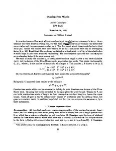
GAGGA counts in HSV1 - 152261 bps
20
’hsv1.gagga’
15
10
5
0
0
FIG. 11.
50
100 window position (800 bps)
150
GAGGA count in a sliding window of size 800bps of the whole HSV1 genome.
200
EFFICIENT DETECTION OF UNUSUAL WORDS
91
The inferred choices of E and N automatically satisfy the rst two assumptions above. The concave ˆ ¡ p) ˆ which appears in the denominator term N w of the above fraction is maximum for product p(1 pˆ 5 1=2, so that, under the realistic assumption that pˆ µ 1=2, the third assumption is satis ed. Thus Z increases with decreasing pˆ along an arc of Tx . In conclusion, once one is restricted to the branching nodes of Tx or their one-symbol extensions, all typical count values E (usually expectation) and their normalizing factors N (usually standard deviation) and other measures discussed earlier in this paper can be computed and assigned to these nodes and their one-symbol extensions in overall linear time and space. The key to this is simply to perform our incremental computations of, say, standard deviations along the suf x links of the tree, instead of spelling out one-by-one the individual symbols found along each original arc. The details are easy and are left to the reader. The following theorem summarizes our discussion.
agac
aggtaa
agttag agaggc
agg
a ga agt
ag
aggagc ag tcc agt
ggc
aaaa
aac
aa
agcccc
agcggc
agccgg agcgag
agcggt
aggcaa
agacta agacag ag tccc
aaaaa a gtcc g
aaa ag g
aaaac aaaggc aaagcg aaacgg
aaaaaa aaaaag aaaacg
aaaaca
aa aca c aagcgg
aaactc aa gca c
agc a
aacggg
aag
aag a
aaac
agcggg
ag gcg g
aaggcg
aaa
agcgg agcgcg
a g ca ct
aggccc
agcg
aggc
agacgc
a gc c
a gc
agccc
agcccg
Theorem 7.3. The set of all d-signi cant subwords of a string x over a nite alphabet can be detected in linear time and space.
aa ca ca
aactc
aactct a a ctcg
acgggc
acg ttc a c ga
aacctc acgccg
aac ccg
acgccc
acgcc
aacc
aac cgc
a cg c
a cg
acg cac
acgctc
acg ac a cga tg
ac g a cg a cg ac t
acac
a ca ca c
a ca gtc aca gcc
accccg gccgc gccgtc
gccag
gccatc
gcct ct gcctgt gcct t c
g c g gg gcggc
actcgc
gcccga
gcccgc
gcccgg
a ctcgg
gccccc gcccac
g ccccg
gccgcg gcc caa
g ccgcc
gccggc gcc aga g cca gt
gcgggg gcg gga g cgg ct gcggtg
g cgg
gccgg gcggt
gcct
gcc
g cca
gccga
gccgaa
gccca
atg
gc ccc
gccct t
gccg
gccgag
a ctc g
a tgg cc
atga cg gccc
a ct gc g
gccggt
a ctgg c
at
gccgga
ac tc
atgctt
actact actcta
gcgggc
ccg aca
gcggcg
acta
acc tcc
a cta gc
gcggcc
ac t
acccgc
acc
accacc
gcccg
ac
accc
acccc
accccc
aca
acag
acaggc
acaccc
a ca tgc
g cg cg c
gc gcg gcgcaa
gcgcc gcgtg
g cgt
gcgtcc
gcaaaa
g cgccc
gctcca
gc tgct gctgcg
gct g c
g ggcc
gggcg gg gca g
ggggg
ggggc gg gag c
gcgtgc gcgtgg gcacag
gggccg gggcgc
g g g cg g g gg gg g
gggggc
ggggga ggggcg ggggcc gg cccc
ggcccg ggccca
gggtcg
ggggag gggagg ggggtc
g gg g
gggag
g ca ca t gggccc
gc aca
gct ct c
gggcgt
g ctc
g ca cta gcacgc
gcagcc
gca c
gcttgc
gggc
gg g
gcgcgg
gcgccg gcgcca
caa g
gggggt
gct
gcaagc
gcgagt
gca
ggccct
gcg
gcgc
gc
ggccag
g g cg g
gtccgg gtgggg
gtcgcg gagt
gagg gagact
gtgggc gtggc gagccg
gaggag gagtta
gtg gc t
gagcgg gagcgc
gtt cgc gt t ccc
gagcg
gaggcc
gttc
gtggcg
gtggg
gtcagg
gtgg
gttaga gag c
gag
g ct cga
gtcaaa
gtgcgc
g tct cc
gtccgc
ggacag
ggagga g tccca
gtca
gtc
t
ggccga
ggcggt ggtggc
ggtcag
ggagcg gt ccg
gt
g taa cc
ggc ggg gg cggc
ggtcgc
ggctcc
g gt c
ggta ac
gtcc
gtg gt
ggcgcc
ggcacg
ggcaag
ggcagc
ggcgtg
ggtccg
ggca
ggag ggaacc
gg a
ggccgg ggcgcg
ggtggg
gg t
ggcgc
ggtgg
ggc gg
ggcg
ggc cg
ggccgc
gg ccc
ggcc
g acga c
gacgcc
g ag ct c
cccgag
cccacg
cccgcg
cccggc
cccggg
ga cg at cccgcc
cccccc cccccg ccc cgc cc ca a a
ccca ac ccgggc
ccgggg
ccggc
ccggca
c cggg
ccggcg ccgcgg
ccgg
ccccaa
cccagg
ccca
cccttt
ccccg
ccccca
gacagg gacagc cccgg
cccgc
cccaa
ccccgg
g act ag
ccccc
ccggcc
gact
ccg c
cccc c cc
ga c ga gactgg
aac gcc
g atgac
ccggtg
gaa
gaaaac
ccggac
ga
gacg gacag
gac
ccgcca
ccgccg
ccgcac
ccg aaa
ccgccc ccgaga
ccgacg
ccgcct
ccgag
ccg a c
ccg
ccgtc
cc
ccgcc
ccgcgt
gc cc g
cc gc
ccaa
cca
c cag tg
ccaccc
cca ac
ccgagc
cc ga gt cca gac ccagag
c cag gt
ccaa a a
ccaacc
cca act ccacgc
ccacg
cac c
ccacgg
aga cc
cc ag
cct ctg c ctcc a cgggc
cct gt c
c gg g g cgg ga g
cgggcc cgggcg
cggggc cggggg cgg cgg
cggcgc cggtcc
cggcac
cggcc
c ggcg
cggt
cggtc
cggg
cggc
cgga
cgggca
ccttct
cctc
cct
cg gtca
cgcggg cgcggc
cggaca
cggaac
cggtgg
cgcggt
cgcgg
cgcgcg
cgca
cgccgc
cgccgg cgcctc
cgccg cgccc cgctgc
cgcccc
cgccag
cgtccg cgagac
cgccat
c gac tg
caaaa
cgccca
cgcccg
cgagt
cga cga
caaact
cg a g tt cg ag tc
caaaaa caa aa c
caa ccg
caactc cagacg
caac
cagagg
aga c
cagg
cagg ta cagt cc
cagt
cagcc c
caggca
caa
cgcca
cgcct
cga c
caaa ca agca
cgagcc
c gag
cgcct t
cgtccc
cgtggg
cgtcc
cg tt cc
cgaaaa cg atga
cag
cgct ct
caggag
c ga
c g tg
cgtgcg
cg cc
cg ct
cgt
ca
cg caaa
cgcaca
cgccgt
cgc
cg
cg cgcc cgccga
cg cgc cgcgtc
cgcg
cgcgca
cgg
cggccg
c ctt
ccacgt
cggcgt
ccttta
cggcca
ccatcg
cggccc
c catg g
at cc
cta
ctt
c at gc g ctac
ctcg
ct
c
ctct ct cca
cacggg
cacgtt catgct
cac gca
cacgct
c atgg c
ct tg cc
cttgtt ctactc ctacca ctcgcc
cttctt cttg
c t
cacacc
c aca tg c aca g t
catg
cat
cac g
ca tcg c
cacgcc
c acc cc
cactac
ctttaa
cacgc
caca
cagtgg
c ac
c ct gg a
ctctg
ctctac
ct ctg c
ctctgt
ctctct ctccat ctcca c
ctgctg ctgcgc
ctgc
ctgcac
ctgtc ctggcc
ctg
ctg tca
tccg
tccgcg
tccggg
ctgtct tccgac
tcca tg tcc a cc tccc
t
tcca cg t ccca
tcccaa tcccag
tcaaac tgcgc
tcagga tg cac g
tt a ttg
tt
ttc
tgc t
t gcctg
tggg
tctcca
tgcttg tgc tgc
tggccg
gt
tggcc
tttaaa t
tggc
tgc
tgg t gacga
tggccc
tcttgt t ac
tg
tctgtc tctctg tgcgcg
t ctc
tgcgcc
tctacc
t cgcct tcgct g
tctg ca
tggggg
tctg
tgggcc
tcggaa
tggcgg
tct
tcgc
tcg
tcgcgg
tcgcg
tcgcgc
tcccga tc
tgtc
tgttcg
ttaaag
tggctc
tgtcaa tgtctc
ttagac ttgcct
ttgttc ttcttg ttcgct t t cccg
taaagc
t aa
ta
tag
t
ac
taacct tagcga
tagaca tactcg taccac
FIG. p 12. Verbumculus 1 Dot on window 0 ( rst 800bps) of HSV1, under score Zw 5 ( f w ¡ (n ¡ ˆ ˆ ¡ p) ˆ (frequencies of individual symbols are computed over the whole genome). 1) p)= (n ¡ jw j 1 1) p(1
jwj 1
92
APOSTOLICO ET AL.
8. SOFTWARE AND EXPERIMENTS The algorithms and the data structures described above have been coded in C++ using the Standard Template Library (STL), a clean collection of containers and generic functions (Musser and Stepanov, 1994). Overall, the implementation consists of circa 2,500 lines of code. Besides outputting information in more or less customary tabular forms, our programs generate source les capable of driving some graph drawing programs such as Dot (Gansner et al., 1993) or DaVinci (Frohlich and Werner, 1995) while allowing the user to dynamically set and change visual parameters such as font size and color. The overall facility was dubbed Verbumculus in an allusion to its visualization features. The program is, however, a rather extensive analysis tool that collects the statistics of a given text le in one or more suf x trees, annotates the nodes of the tree with the expectations and variances, etc. Example visual outputs of Verbumculus are displayed by the gures which are found in the paper. The whole word terminating at each node is printed in correspondence with that node and with a font size that is proportional to its score; underrepresented words that appear in the string are printed in italics. To save space, words that never occur in the string are not displayed at all, and the tree is pruned at the bottom. Figures 8–10 show an application to the rst 512 bps of the mitochondrial DNA of the yeast under scores d, Z and p ˆ Z 5 ( f w ¡ (n ¡ jw j 1 1) p)= V ar (Z jw). Figures 11–14 are related to computations presented in (Leung et al., 1996) in the context of a comparative analysis of various statistical measures of over- and underrepresentation of words. It should be clari ed that here we are only interested in the issue of effective detection of words that are unusual according to some predetermined score or measure the intrinsic merits which are not part of our concern. The histograms of Figures 11 and 13 represent our own reproduction of computations and tables originally presented in (Leung et al., 1996) and related to occurrence counts of few extremal 4- and 5-mers in some genomes. Such occurrences are counted in a sliding window of length approximately 0.5% of the genomes themselves. We use for a concrete example the counts of the occurrences of GAGGA and CCGCT, respectively, in HSV1 (circa 150k bps). Peaks are clearly visible in the tables, thereby denouncing local CCGCT counts in HSV1 - 152261 bps
20
’hsv1.ccgct’
15
10
5
0
0
FIG. 13.
50
100 window position (800 bps)
150
CCGCT count in a sliding window of size 800bps of the whole HSV1 genome.
200
EFFICIENT DETECTION OF UNUSUAL WORDS
93 g
gggggc
gg gg g
gg gg gg gggggt
gggg
ggggc
ggggc
ggggtg
g gg ct g gggcc
gggcca
gggccg
ggc gcc
gg gc gg
gggcgc
gggcg
gggc
gggcgt
gggaac
gggact gggtgg
gg gt tc gggtg
g gg t
gggacg
gggac
ggga
ggg
ggccag
gg gtgt gg ct t g ggctg
ggcc at ggcccg
ggcca
ggccca
gg ctgc
ggcccc
ggccg
gg cc
g g cc c
gcc ggc
ggcgca
g g cc g g
ggcgcg
ggcg c
ggcgcc gg cg gg
g gc g g
gg cg gc ggacgg
ggacg
ggacgc
ggcgtc
ggcgtg
ggcgt
ggcg
ggcaag
ggcgag
gg c
ggag
gg act
gga ct c
ggaccg
ggaacg
ggactg
ggagcc
gga
gga c
gg
g ga gg t ggttcc
ggagac
gg ttac
gtt g
gg tgg t
gctcc gctt
g cta gt
gctcct gctccc
gcttta
gc cact gccacc
gct
gg gg t t gg gtg t
g gtga a gctgtc
g c tg
gctgcc
g gtg
g gta ga
gcttgc
ggt
gcca gt gccac
gccaca
gcca
gcccgt gcccgg
gcccac
gcccgc
gcccg gccgc
ccg gcg
gccgct
gccgcc
g cggg g
gccttt
gcgggc gcgggt
gcggg
g cgg cg
gcg gc
gcggcc
gcgg
gccccg
gccccc
gccggg
gcct
gcca gt
gcctgt
gccg
gcccc gcggac
gcc
gccc
gcgcac
gcgcag
gcgca
gc ggtt
g cgc gc
gcgctc
gcgc
gc gcg
gcgcga
g cg ccc
gcg
g cga ac gcgatg gcgagt gcgtg
gc gtgc
gcgtct
g cagca
gcag
gcgt
gcgacc
gcgtgg
gcga
gc
gtcg
gtccgg
gcacg
gtcgtc gtcgga
gtctaa gtctcg
gtct
gt catc
gcagcg
g catgt
gtc
gc agc
gcagag gcacgc
gca agc
gcacgg
g ca
gtctgg
gtgcgg
gtggta
gtgc
gtgcg
gtgg
gtgggc
gtggag gtgccg
gtgcg t
gtgt
gtgaaa gt tacc gtt t
g tag ag gt agtg
gtttt c
gactcg
ga ctg t
g a cc
gacaga
g aca g
g t tt tg
gtttt
gacg gact
gac
gtgcag
gtg ctt
gtgtgt
g t g ttt
gttt ga gacgcg
g ttgg g
gaccgc gacccc
ttg
t gga
gacggc
gttccg
gtg
gt
gacagg
g a a cgt
g aac
gaaggc
ga aa cc gagc
ga a
ga
gagt
ag g
gatggc
gaacaa g agc ca gagcgt
g agc ac
gagttg
gagtt g agta g
gagttt
gaggtt
gagaca gaggcg
ga gg
gaga
ccg agt
ccgt cca gt c
ctgtcc
ctgtc
ctggcg
ctgtgc
ctggcc ctcggg ctcggc
ctcctg
ctcgct
ccgggc ccgggg ccgcga
cgc cgg
cc gcg c ccgccg
ccgct
ccgccc ccgcct
ccgctc
ccgttt cactg c cac ccg
c ccg
cccgtg
cccgtt
cccg t
cccggg
cc aa ca
ccacag
cccgga
cca c
cca gt g
cccac
c cc
cc
ctcccg
ccggcg
ccgcc
ccacgc
c cg
cca
ccggcc
ctcccc
ccggc
ccgcca
ccgc
cttttt
ctttaa
ccgctt
ccgg
ctccc
ctcctc
ctcgg
ccggg
cttt
ct agtc
t c gc ca
ccggac
cta act
ct gtct
ctggga ctgccc
ctcct
ccgcg
c ta
ctgacc
ctg cc
cccacc
ctt
ct
c tg g
ctcg
ctcc
cccacg
ctc
cttgcc
ctg
ctggc
ccgtgg
ctgt
gagagc
cccgg
cccgcc
cccgct
cccgc
ccc gc g
cctttt
ccccca
ccccgg
ccccac
ccccg cctggg
ctc ac g
cggcca
ccc cgc
cg gcc
cggccg
cggccc cggcgg c ggcg c
cg gcg cggacg
cg gc
cccccc
cggcgt
cct
cctg
cctccc
c cc cc g
ccccc cctgtc
cc cc
cggacc
cgggaa
cggggt
cgggg
cgggcc cgggcg
cggg
c gg
cggggg cggggc
cgga ct
cggac
cggtt g
cgggc cg ggtt
cg ggc t
cgtcat
cgtggg cgtgcc
cgtgg
cgcgga
cgtgca cgcgg
cgtt tt
cgtgc
cgcggc
cgcg
cg t
cgtg
cgtctg
cgtc
cgtcgg
cgtcg
cgtcgt cg tgg a cgcg gg
cga aca c gag t cgaccc
cgatgg
ca gt c g
cag
ca gc
ca gag cagg
cgcgct
cgcacg
cgctcc
cgcgca
cgcgcc
cgctag
cgcg at
cgcttt
cgcgac
cgccc cgccgc
cgcccg
cgcccc
cgccac
cgct
cgcc cga
cgcgcg
cgcctt
cgc
c g ca
cgcagc
cgcga
cgc gc
cg
cga gtt
c ga g ta
cagcag ca gcg a
cagaga cagagg ca ga gc ca gg ca caggtg
c at gg a catgtg caccgg
ca ctg g
c aag
acg ccc
caagaa ca ag ca
tgtc
tgtccg
caa ca g
cacggc
c a cg caca gg
caccgc
catg
cat cgt
caa
c ac
caccg
cat
ca
t gt gcg
tgtttt
t g tg tt
tg g ag tggc
tgg ag a
tggagc
tggcgc
t gg agg
tg ctt g
tccg tcc tc
tcg tcatcg
tgggcc
tgggc tggggg
tgcgg t
tgccgg
tgcgcg
tgcgtg
tgcc ac
ct cgag
tcctga
tcctcc
tccc tc g tc
tccccc
tcgg t cgct a
tcgtcg
tcta ac
tcccg c
tcgt ca ct ggac
t tg gg
tta
t ta cc t
ttaaag
tttaaa tt tg
ttt
tttt tagagt tt tcg g
tacct g tag
ta
t agt
taa
ta actc agtc
taaagg agtt
agt
agtagt a gtgct agccac
ag
agc
a gca agcg
aga
tcggga
agaagg ag acag agag
tcggcg
tcggc
tt ggc g
ttggga tt g ggg
ttgcct ttgcgc
ttcggc
t tccga
ttgaca ttgc
ttg
ttc tt
tcggcc
tctggc
tctcgg
tct
tcct
gt accg
tgcctg
tgcc tg ca g a
tg gg ac
t ga ca g tgcccg
t g cg
tccggc
tgc
tgac
tga
tg gtag
tgaaac
tgggcg
tggccg
tggg
tggcgg
tggcg
tgtg
tgt tgg
tg
tgtcta
tttgac t tt ggg tttg cg
t tt tg g
ttttg
ttttg c
ttttcg
tttttt
ttttt
tttttg
ta gtgc
tagtct ag tcg t agtct c
agttgg
agt ttg ag cagc
a g ca tg a gca cg
agcgaa agcgtg
agagag
agagcg
ag agc
agagca
agagtt
aggcgg
agaggc
aggcga
aggc
aggcg
aggcaa
ag g agggcc
gg ta
at cgtc
a ggtg a atggcg
a tg ga g
ac ct g
actg
acaaga
a ac
aa g
a cag gc
a ca g g t
aagaag aa gg
accgcc
ac cgct
aactcg
aagcat aaa
cta gc c
aca gg
accgcg
ac ctg g
a cca a c a ac gt g a a ca
aaccaa
aa
actcgg actggc
actgtg
acagag accggc
accg
a ca g accccc
a ca
acc
accgc
a cg act
ac
acgtgg acggcg
acgccg
acgcc
a c gc
acgccc
tgg a
a tg tg c
acgcgg
atg
at
aggtta
aacaag aacaga aaggcg aagggc
aaaggg
aaacca
FIG. p 14. Verbumculus 1 Dot on window 157 (800bps) of HSV1, under score Zw 5 ˆ 1) p)= V ar(Z jw ) (frequencies of individual symbols are computed over the whole genome).
(fw ¡
(n ¡
jw j 1
departures from average in the behavior of those words. Such peaks are found, e.g., in correspondence with some initial window position in the plot drawn for GAGGA and more towards the end in the table of CCGCT. Note that, in order to nd, say, which 5-mers occur with unusual frequencies (by whatever measure), one would have to rst generate and count individually each 5-mer in this way. Next, to obtain the same kind of information on 6-mers, 7-mers or 8-mers, the entire process would have to be repeated. Thus, every word is processed separately, and the count of a speci c word in a given window is not directly comparable to the counts of other words, both of the same, as well as different length, appearing in that window. Such a process can be quite time consuming, and the simple inspection of the tables at the outset may not be an easy task. For instance, the plain frequency table of yeast 8-mers alone (van Helden et al., 1998) requires almost 2 megabytes to store. Figures 12 and 14 display trees (suitably pruned at the bottom) produced at some of the peak-windows in the corresponding histograms. Not surprisingly, Verbumculus enhances the same words as found in the corresponding table. Note, however, that in both cases the program exposes as unusual a family of words related to the single one used to generate the histogram, and sometimes other words as well. The
94
APOSTOLICO ET AL.
words in the family are typically longer than the one of the histogram, and each actually represents an equally, if not more surprising, context string. Finally, Verbumculus nds that the speci c words of the histograms are, with their detected extensions, overrepresented with respect to the entire population of words of every length within a window, and not only with respect to their individual average frequency.
9. ACKNOWLEDGMENTS We are indebted to R. Arratia for suggesting the problem of annotating statistical indices with expected values, to M. Waterman for enlightening discussions and to M.Y. Leung for providing data and helpful comments.
REFERENCES Aho, A.V., Hopcroft, J.E., and Ullman, J.D. 1974. The Design and Analysis of Computer Algorithms, Addison-Wesley, Reading, Mass. Aho, A.V. 1990. Algorithms for nding patterns in strings, in Handbook of Theoretical Computer Science. Volume A: Algorithms and Complexity, (J. van Leeuwen, ed.), Elsevier, 255–300. Apostolico, A. 1985. The myriad virtues of suf x trees, Combinatorial Algorithms on Words, (A. Apostolico and Z. Galil, eds.), Springer-Verlag Nato ASI Series F, Vol. 12, 85–96. Apostolico, A., Bock, M.E., and Xuyan, X. 1998. Annotated statistical indices for sequence analysis, (invited paper) Proceedings of Compression and Complexity of SEQUENCES 97, IEEE Computer Society Press, 215–229. Apostolico, A., and Galil, Z. (eds.) 1997. Pattern Matching Algorithms, Oxford University Press. Apostolico, A., and Preparata, F.P. 1996. Data structures and algorithms for the string statistics problem, Algorithmica, 15, 481–494. Apostolico, A., and Szpankowski, W. 1992. Self-alignments in words and their applications, Journal of Algorithms, 13, 446–467. Brendel, V., Beckman, J.S., and Trifonov, E.N. 1986. Linguistics of nucleotide sequences: morphology and comparison of vocabularies, Journal of Biomolecular Structure and Dynamics, 4, 1, 11–21. Chen, M.T., and Seiferas, J. 1985. Ef cient and elegant subword tree construction, 97–107. In Apostolico, A., and Galil, Z., eds., Combinatorial Algorithm on Words. Series F, Vol. 12, Springer-Verlag, Berlin, NATO Advanced Science Institutes. Crochemore, M., and Rytter, W. 1994. Text Algorithms, Oxford University Press, New York. Frohlich, M., and Werner, M. 1995. Demonstration of the interactive graph visualization system Davinci, In Proceedings of DIMACS Workshop on Graph Drawing ‘94, Princeton (USA) 1994, LNCS No. 894, R. Tamassia and I. Tollis, Eds., Springer Verlag. Gansner, E.R., Koutso os, E., North, S., and Vo, K.-P. 1993. A technique for drawing directed graphs. IEEE Trans. Software Eng. 19, 3, 214–230. van Helden, J., Andrè, B., and Collado-Vides, J. 1998. Extracting regulatory sites from the upstream region of yeast genes by computational analysis of oligonucleotide frequencies. J. Mol. Biol., 281, 827–842. Leung, M.Y., Marsh, G.M., and Speed, T.P. 1996. Over- and underrepresentation of short DNA words in herpesvirus genomes, Journal of Computational Biology 3, 3, 345–360. Lothaire, M. 1982. Combinatorics on Words, Addison Wesley, Reading, Mass. Lyndon, R.C., and Schutzemberger, M.P. 1962. The equation a M 5 bN c P in a free group, Mich. Math. Journal 9, 289–298. McCreight, E.M. 1976. A space economical suf x tree construction algorithm, Journal of the ACM, 25, 262–272. Musser, D.R., and Stepanov, A.A. 1984. Algorithm-oriented generic libraries, Software—Practice and Experience 24, 7, 623–642. Schbath, S. 1997. An Ef cient Statistic to Detect Over- and Under-represented words, J. Comp. Biol. 4, 2, 189–192. Waterman, M.S. 1995. Introduction to Computational Biology, Chapman and Hall. Weiner, P. 1973. Linear pattern matching algorithm, 1–11. In Proceedings of the 14th Annual IEEE Symposium on Switching and Automata Theory. IEEE Computer Society Press, Washington, D.C.
Address correspondence to: Alberto Apostolico Department of Computer Sciences Purdue University West Lafayette, IN 47907 E-mail:
[email protected]