Efficient Linear Array for Multiplication in GF (2m ) Using a Normal Basis for Elliptic Curve Cryptography Soonhak Kwon1 , Kris Gaj2 , Chang Hoon Kim3 , and Chun Pyo Hong3 1
Inst. of Basic Science and Dept. of Mathematics, Sungkyunkwan University, Suwon 440-746, Korea
[email protected] 2 Dept. of Electrical and Computer Engineering, George Mason University, University Drive, Fairfax, VA 22030, USA
[email protected] 3 Dept. of Computer and Information Engineering, Daegu University, Kyungsan 712-714, Korea
[email protected],
[email protected]
Abstract. We present a new sequential normal basis multiplier over GF (2m ). The gate complexity of our multiplier is significantly reduced from that of Agnew et al. and is comparable to that of Reyhani-Masoleh and Hasan, which is the lowest complexity normal basis multiplier of the same kinds. On the other hand, the critical path delay of our multiplier is same to that of Agnew et al. Therefore it is supposed to have a shorter or the same critical path delay to that of Reyhani-Masoleh and Hasan. Moreover our method of using a Gaussian normal basis makes it easy to find a basic multiplication table of normal elements. So one can easily construct a circuit array for large finite fields, GF (2m ) where m = 163, 233, 283, 409, 571, i.e. the five recommended fields by NIST for elliptic curve cryptography. Keywords: Massey-Omura multiplier, Gaussian normal basis, finite field, elliptic curve cryptography, critical path delay.
1
Introduction
Finite field multiplication finds various applications in many cryptographic areas such as ECC and AES. Though one may design a finite field multiplier in a software implementation, a hardware arrangement has a strong advantage when one wants a high speed multiplier. Moreover arithmetic of GF (2m ) is easily realized in a circuit design using a few logical gates. A good multiplication algorithm depends on the choice of a basis for a given finite field. Especially a normal basis is widely used [5,10,11] because it has some good properties such as simple squaring. A multiplication in GF (2m ) can be classified into two types, a parallel (two dimensional) [4,5,8,10] and a sequential (linear) [1,3,9,11] architectures.
Though a parallel multiplier is well suited for high speed applications, ECC requires large m for GF (2m ) (at least m = 163) to support a sufficient security. In other words, since the parallel architecture has an area complexity of O(m2 ), it is not suited for this application. On the other hand, a sequential multiplier has an area complexity of O(m) and therefore is applicable for ECC. Since it takes m clock cycles to produce one multiplication result using a sequential multiplier, it is slower than a parallel multiplier. Consequently reducing the total delay time of a sequential multiplier is very important. A normal basis multiplier of Massey and Omura [7] has a parallel-in, serialout structure and has a quite long critical path delay proportional to log2 m. Agnew et al. [1] proposed a sequential multiplier which has a parallel-in, parallelout structure. It is based on the multiplication algorithm of Massey and Omura, however the critical path delay of the multiplier of Agnew et al. is significantly reduced from that of Massey and Omura. Recently, Reyhani-Masoleh and Hasan [3] presented two sequential multipliers using a symmetric property of multiplication of normal elements. Both multipliers in [3] have roughly the same area complexity and critical path delay. These multipliers have the reduced area complexity from that of Agnew et al. with a slightly increased critical path delay. In fact, the exact critical path delay of the multipliers of Reyhani-Masoleh and Hasan is difficult to estimate in terms of m and is generally believed to be slightly longer or equal to that of Agnew et al. For example, for the case of a type II ONB, the critical path delay of Reyhani-Masoleh and Hasan [3] is TA + 3TX while that of Agnew et al. [1] is TA + 2TX , where TA , TX are the delay time of a two input AND gate and a two input XOR gate, respectively. However since we are dealing with a sequential (linear) multiplier, even a small increment of critical path delay such as TX results in a total delay of mTX where m is the size of a field. Our aim in this paper is to present a sequential multiplier using a Gaussian normal basis in GF (2m ) for odd m. Since choosing an odd m is a necessary condition for cryptographic purposes and since a low complexity normal basis is frequently a Gaussian normal basis of type (m, k) for low k, our restriction in this paper does not cause any serious problem for practical purposes. In fact all the five recommended fields GF (2m ) by NIST [16] for ECC where m = 163, 233, 283, 409, 571 can be dealt using our Gaussian normal basis, and the corresponding circuits are easy to construct if one follows a simple arithmetic rule of a Gaussian normal basis. We will show that the area complexity of our sequential multiplier is reduced from that of the multiplier of Agnew et al. [1] and thus comparable to that of the multiplier of Reyhani-Masoleh and Hasan [3]. Moreover the critical path delay of our multiplier is same to that of Agnew et al. and therefore is believed to be shorter or equal to that of Reyhani-Masoleh and Hasan.
2
Review of the Multipliers of Agnew et al. and Reyhani-Masoleh and Hasan
Let GF (2m ) be a finite field with characteristic two. GF (2m ) is a vector space of 2 m−1 dimension m over GF (2). A basis of the form {α, α2 , α2 , · · · , α2 } is called a
normal basis for GF (2m ). It is well known [6] that a normal basis exists for all i m ≥ 1. Let {α0 , α1 , · · · , αm−1 } be a normal basis in GF (2m ) with αi = α2 . Let αi αj =
m−1 X
(s)
λij αs ,
(1)
s=0
(s)
where λij is in GF (2). Then for any integer t, we have t
αi αj = (αi−t αj−t )2 =
m−1 X
(s)
λi−t,j−t αs+t =
m−1 X
(s−t)
λi−t,j−t αs ,
(2)
s=0
s=0
where the subscripts and superscripts of λ are reduced (mod m). Therefore comparing the coefficients of αs , we find (s)
(s−t)
(s)
(0)
λij = λi−t,j−t .
(3)
In particular, we have λij = λi−s,j−s . (4) Pm−1 Pm−1 Letting A = i=0 ai αi and B = j=0 bj αj in GF (2m ), we have the multipliPm−1 cation C = AB = s=0 cs αs where C=
X
ai bj αi αj =
i,j
X
ai bj
m−1 X s=0
i,j
(s)
λij αs =
m−1 X s=0
X (s) ( ai bj λij )αs .
(5)
i,j
Fig. 1. A circuit of Agnew et al. in GF (25 )
Therefore, using (4), we have the coefficients cs of C = AB as X X X (s) (0) (0) cs = ai bj λij = ai bj λi−s,j−s = ai+s bj+s λij , i,j
i,j
(6)
i,j
where the subscripts of a, b and λ are reduced (mod m). The circuit of Agnew et al. [1] is a straightforward realization of the above equation with the information
(0)
of the m by m matrix (λij ). When there is a type II ONB (optimal normal basis), (0)
it is easy to find λij as is explained in [1]. That is, (0)
λij = 1 iff
2i ± 2j ≡ ±1 (mod 2m + 1).
(7)
Figure 1 shows the circuit of Agnew et al. for the case m = 5 where a type II (0) ONB is used. For arbitrary finite field, finding λij may not be so easy. However (0)
if we have a Gaussian normal basis, one can easily find λij by following a simple arithmetic rule. A Gaussian normal basis and a type II ONB will be discussed briefly in the following sections. Recently, Reyhani-Masoleh and Hasan [3] suggested a new normal basis multiplication algorithm which significantly reduces the area complexity compared with the multiplier of Agnew et al. They used ααi instead of αi αj and wisely utilized the symmetric property between ααi and ααm−i . In fact they proposed two sequential multiplication architectures, so called XESMPO and AESMPO [3]. Since the hardware complexity of AESMPO is higher than that of XESMPO and both architectures have the same critical path delay, we will sketch the idea in [3,4] for the case of XESMPO. In [3,4], the multiplication C = AB is expressed as X
ai bj αi αj =
m−1 X
=
m−1 X
ai bi αi+1 +
m−1 XX
ai bi αi+1 +
m−1 XX
i
i=0 j6=i
i=0
i,j
ai bj (ααj−i )2
(8) 2i
ai bj+i (ααj ) .
i=0 j6=0
i=0
When m is odd, the second term of the right side of the above equation is written as m−1 ν m−1 X X m−1 XX i i ai bj+i (ααj )2 , (9) ai bj+i (ααj )2 + i=0 j=m−ν
i=0 j=1
and when m is even, it is written as ν m−1 XX
i
ai bj+i (ααj )2 +
m−1 X X m−1
i
ai bj+i (ααj )2 +
i
ai bν+1+i (ααν+1 )2 , (10)
i=0
i=0 j=m−ν
i=0 j=1
m−1 X
⌊ m−1 2 ⌋,
i.e. m = 2ν + 1 or m = 2ν + 2. Also the second term of (9) where ν = and (10) is written as m−1 X X m−1
ai bj+i (ααj )2 =
ν m−1 XX
ai bm−j+i (ααm−j )2
=
ν m−1 XX
ai+j bi (ααm−j )2
ν m−1 XX
ai+j bi (ααj )2 ,
i
i
i=0 j=1
i=0 j=m−ν
i=0 j=1
=
i=0 j=1
i
i+j
(11)
where the first (resp. second) equality comes from the rearrangement of the summation with respect to j (resp. i) and all the subscripts are reduced to (mod m). Therefore we have the basic multiplication formula of Reyhani-Masoleh and Hasan depending on whether m is odd or m is even as AB =
m−1 X
ai bi αi+1 +
i=0
ν m−1 XX
i
(ai bj+i + aj+i bi )(ααj )2 ,
(12)
i=0 j=1
or AB =
m−1 X i=0
ai bi αi+1 +
ν m−1 XX
i
(ai bj+i + aj+i bi )(ααj )2 +
m−1 X
i
ai bν+1+i (ααν+1 )2 .
i=0
i=0 j=1
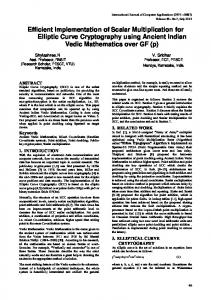
(13) Using these formulas, they derived a sequential multiplier where the gate complexity is significantly reduced from that of [1]. The circuit of the multiplier is shown in Figure 2 for m = 5 where a type II ONB is used.
Fig. 2. A circuit of Reyhani-Masoleh and Hasan in GF (25 )
3
Gaussian Normal Basis of Type k in GF (2m)
We will briefly explain basic multiplication principle in GF (2m ) with a Gaussian normal basis of type k over GF (2) (See [6,12].). Let m, k be positive integers such that p = mk + 1 is a prime 6= 2. Let K = hτ i be a unique subgroup of order k in GF (p)× . Let β be a primitive pth root of unity in GF (2mk ). The following element k−1 X j βτ (14) α= j=0
is called a Gauss period of type (m, k) over GF (2). Let ordp 2 be the order of 2 (mod p) and assume gcd(mk/ordp 2, m) = 1. Then it is well known [6] that i α is a normal element in GF (2m ). That is, letting αi = α2 for 0 ≤ i ≤ m − 1, m {α0 , α1 , α2 , · · · , αm−1 } is a basis for GF (2 ) over GF (2). It is called a Gaussian normal basis of type k or (m, k) in GF (2m ). Since K = hτ i is a subgroup of order k in the cyclic group GF (p)× , the quotient group GF (p)× /K is also a cyclic group of order m and the generator of the group is 2K. Therefore we have a coset decomposition of GF (p)× as a disjoint union, GF (p)× = K0 ∪ K1 ∪ K2 · · · ∪ Km−1 ,
(15)
×
i
where Ki = 2 K, 0 ≤ i ≤ m − 1, and an element in GF (p) is uniquely written as τ s 2t for some 0 ≤ s ≤ k − 1 and 0 ≤ t ≤ m − 1. For each 0 ≤ i ≤ m − 1, we have k−1 k−1 X s X s k−1 X k−1 X s X k−1 X t i k−1 t i t−s i β τ (1+τ 2 ) . (16) βτ ααi = β τ (1+τ 2 ) = βτ 2 = s=0
s=0 t=0
s=0 t=0
t=0
From (15), there are unique 0 ≤ u ≤ k − 1 and 0 ≤ v ≤ m − 1 such that 1 + τ u 2v = 0 ∈ GF (p). If t 6= u or i 6= v, then we have 1 + τ t 2i ∈ Kσ(t,i) for some ′ 0 ≤ σ(t, i) ≤ m − 1 depending on t and i. Thus we may write 1 + τ t 2i = τ t 2σ(t,i) for some t′ . Now when i 6= v, ααi =
k−1 X X k−1
=
k−1 X X k−1
βτ
s
(1+τ t 2i )
=
k−1 X X k−1
βτ
s
′
(τ t 2σ(t,i) )
s=0 t=0
s=0 t=0
β
′
τ s+t 2σ(t,i)
=
k−1 X
α
2σ(t,i)
=
(17) ασ(t,i) .
t=0
t=0
t=0 s=0
k−1 X
Also when i = v, ααv =
k−1 X X k−1
βτ
s
(1+τ t 2v )
=
X X k−1
+
k−1 X
s=0 t=0
=
X X k−1
βτ
s
′
(τ t 2σ(t,v) )
β
′
1=
s=0
t6=u s=0
k−1 X
βτ
s
(1+τ u 2v )
s=0
t6=u s=0
τ s+t 2σ(t,v)
+
X t6=u
α
2σ(t,v)
+k =
X
(18) ασ(t,v) + k.
t6=u
Therefore ααi is computed by the sum of at most k basis elements in {α0 , α1 , · · · , αm−1 } for i 6= v and ααv is computed by the sum of at most k − 1 basis elements and the constant term k ≡ 0, 1 ∈ GF (2).
4 4.1
New Multiplication Algorithm Using a Gaussian Normal Basis in GF (2m) for m Odd (s)
Symmetry of (λij ) and (λij )
Efficient implementation of ECC over a binary field GF (2m ) requires that m is odd, or more strongly m is prime. These conditions are necessary to avoid PohligHelllman type attacks. For example, all the five binary fields GF (2m ), m =
163, 233, 283, 409, 571 suggested by NIST [16] for ECDSA have the property that m = prime. Therefore it is not so serious restriction to assume that m is odd for a fast multiplication algorithm if one is interested in this kind of applications. For odd values of m, it is well known [15] that a Gaussian normal basis of type k or (m, k) always exists for some k ≥ 1. Since mk + 1 is a prime with m = odd, it follows that k is even. Thus it is enough to study the multiplication in GF (2m ) for odd m with a Gaussian normal basis of type k for even k. To derive a low complexity architecture, in view of the multiplication formulas (17) and (18), one should choose a small k, i.e. low complexity Gaussian normal basis. The least possible even k ≥ 1 is k = 2. This is so called a type II ONB (optimal normal basis) or more specifically a type 2 Gaussian normal basis. Among the five binary fields recommended by NIST, m = 233 is the only case where a type II ONB exists. On the other hand, the lowest complexity Gaussian normal basis for the rest of the fields are type 4 Gaussian normal basis when m = 163, 409, type 6 Gaussian normal basis when m = 283, and type 10 Gaussian normal basis when m = 571 (See [12]). i Let {α0 , α1 , · · · , αm−1 } be any normal basis in GF (2m ) with αi = α2 and let m−1 X λij αj , (19) ααi = j=0
where λij is in GF (2). Taking repeated powers of 2 for both sides of the above equation, one finds (s) λij = λi−j,s−j , (20) (s)
(s)
where λij is defined in (1). An explicit table of λij is necessary for construction of the multipliers of Agnew et al. and also of Reyhani-Masoleh and Hasan. (s) Finding λij may not be so easy unless one has a sufficient information on the (s)
given normal basis. Also note that (λij ) is a symmetric matrix but (λij ) is not in general. However, it turns out that (λij ) is a symmetric matrix if a Gaussian normal basis of type k with k even is used. More precisely, we have the following. Lemma 1. If {α0 , α1 , · · · , αm−1 } is a Gaussian normal basis of type k where k is even, then we have (0) λij = λij . Proof. From (20), it is enough to show that λij = λi−j,−j . From the formulas (17) and (18), it is clear that λij = 1 if and only there exist odd pairs of (s, s′ ) (mod k) such that ′ 1 + τ s 2i = τ s 2j , (21) where hτ i is mk + 1. Let way define T To prove λij
a unique multiplicative subgroup of order k in GF (p)× with p = S be the set of all pairs (s, s′ ) (mod k) satisfying (21) and same ′ as the set of all pairs (t, t′ ) (mod k) satisfying 1 + τ t 2i−j = τ t 2−j . = λi−j,−j , it suffices to show that the sets S and T have the same
′
cardinality. Dividing both sides of the equation (21) by τ s 2j , we get ′
′
τ −s 2−j + τ s−s 2i−j = 1.
(22) k
Since the order of τ is k where k is even, we have −1 = τ 2 and therefore k
′
′
τ −s 2−j = 1 + τ 2 +s−s 2i−j .
(23)
Since the map fS : S → T defined by fS (s, s′ ) = ( k2 + s − s′ , −s′ ) and the map fT : T → S defined by fT (t, t′ ) = ( k2 +t−t′ , −t′ ) give one to one correspondence, i.e. fS ◦ fT = id = fT ◦ fS , we are done. ⊓ ⊔ 4.2
Construction of a sequential multiplier and complexity analysis Pm−1 Now from (6) and also from Lemma 1, we have cs of C = i=0 cs αs = AB as cs =
X i,j
(0)
ai+s bj+s λij =
X
ai+s bj+s λij =
m−1 X X m−1
(
j=0
i,j
ai+s λij )bj+s .
(24)
i=0
Let us define an element xst , 0 ≤ s, t ≤ m − 1, in GF (2) as m−1 X
xst = (
ai+s λit )bt+s ,
(25)
i=0
with corresponding matrix X = (xst ). Then the tth column vector Xt of X is Xt = (x0t , x1t , · · · , xm−1,t )T ,
(26)
where (x0t , x1t , · · · , xm−1,t )T is the transposition of the row vector (x0t , x1t , · · · , xm−1,t ). Also the sum of all column vectors Xt , t = 0, 1, · · · , m − 1, is exactly (c0 , c1 , · · · , cm−1 )T ,
(27)
Pm−1 because t=0 xst = cs . Our purpose is to reduce the gate complexity of our multiplier by rearranging the column vectors Xt and reusing partial sums in the computation. Let m − 1 = 2ν and define m by m matrix Y = (yst ) by the following permutation of the column vectors of X as follows; When ν is odd, define Y as (Xν , · · · , X3 , X1 , Xm−1 , Xm−3 , · · · , Xm−ν , Xν−1 , · · · , X2 , X0 , Xm−2 , · · · , Xm−ν+1 ), (28)
and when ν is even, Y is defined as (Xν , · · · , X2 , X0 , Xm−2 , · · · , Xm−ν , Xν−1 , · · · , X3 , X1 , Xm−1 , Xm−3 , · · · , Xm−ν+1 ). (29)
Then the sum of all column vectors Yt , 0 ≤ t ≤ m − 1, of Y with Yt = (y0t , y1t , · · · , ym−1,t )T is same to the sum of all column vectors Xt , 0 ≤ t ≤ m−1, of X which is (c0 , c1 , · · · , cm−1 )T .
To derive a parallel-in, parallel-out multiplication architecture, we will compute the sum of shifted diagonal vectors of Y, instead of computing the sum of column vectors of Y . This can be done from the following observations. In the expression of the matrix Y , there are exactly t − 1 columns between the vectors Xt and Xm−t . Also, sth entry of Xt and s + tth entry of Xm−t have the same terms of ai s in their summands. In other words, from (25), we have m−1 X
xs+t,m−t = (
m−1 X
ai+s+t λi,−t )bs = (
i=0
i=0
m−1 X
ai+s λi−t,−t )bs = (
ai+s λit )bs , (30)
i=0
where the third expression comes from the rearrangement of the summation on the subscript i and the last expression comes from Lemma 1 saying λij = λi−j,−j . Pm−1 Thus xst and xs+t,m−t have the same term i=0 ai+s λit in their expression and this will save the number of XOR gates during the computation of AB. Table 1. New multiplication algorithm
—————————————————————————————————– Pm−1 Pm−1 1. A = i=0 ai αi and B = i=0 bi αi are loaded in m-bit registers respectively. Also intermediate values D0 , D1 , · · · , Dm−1 of the multiplication are all set to zero. 2. For t = 0 to m − 1, do the following; ys,s+t + Ds+t −→ Ds+t+1 ,
(31)
where the above computation is done in parallel for all 0 ≤ s ≤ m − 1.P 3. After mth iteration, we have Di = ci for all 0 ≤ i ≤ m−1, where AB = m−1 i=0 ci αi .
—————————————————————————————————– Let us explain the above algorithm in detail. At the first cycle (t = 0), Ds+1 = Ds + yss are simultaneously computed for all 0 ≤ s ≤ m − 1, i.e. D1 = y00 , D2 = y11 , · · · , D0 = ym−1,m−1 . When t = 1, Ds+2 = Ds+1 + ys,s+1 are simultaneously computed for all 0 ≤ s ≤ m − 1, i.e. D2 = D1 + y01 = y00 + y01 , D3 = D2 + y12 = y11 +y12 , · · · , D1 = D0 +ym−1,0 = ym−1,m−1 +ym−1,0 . Finally, at mth (t = m−1) cycle, Ds = Ds−1 + ys,s−1 are simultaneously computed. That is, D0 = Dm−1 + y0,m−1 = y00 + y01 + · · · + y0,m−1 = c0 , D1 = D0 + y10 = y11 + y12 + · · · + y10 = c1 , ······ Dm−1
······ = Dm−2 + ym−1,m−2 = ym−1,m−1 + ym−1,0 + · · · + ym−1,m−2 = cm−1 . (32)
In other words, for a fixed s, the final value Ds is sequentially computed in the following order Ds+1
m−1 X z}|{ Ds = yss +ys,s+1 + ys,s+2 + · · · + ys,s−1 = ys,s+i = cs . | {z } i=0 Ds+2
(33)
Note that ys−1,s and yss , 0 ≤ s ≤ m − 1, in the equation (32), are from the same column Ys of the matrix Y . Since Y is obtained by a column permutation of a matrix X, we conclude that ys−1,s = xs−1,s′ and yss = xss′ for some s′ depending on s. Moreover from the equation (25), we get m−1 X
xss′ = (
ai+s λis′ )bs′ +s ,
m−1 X
and xs−1,s′ = (
ai+s−1 λis′ )bs′ +s−1 ,
(34)
i=0
i=0
which implies that xs−1,s′ (= ys−1,s ) is obtained by right cyclic shifting by one position of the vectors ai s and bi s from the expression xs,s′ (= ys,s ). Since this can be done without any extra cost, all the necessary gates to construct a circuit from the algorithm in Table 1 are the gates needed to compute the first (i.e. t = 0) clock cycle of the step 2 of the algorithm, Ds+1 = Ds + yss ,
0 ≤ s ≤ m − 1.
(35)
Recall that, for each s, there is a corresponding (because of a permutation) s′ such that m−1 X ai+s λis′ )bs′ +s . (36) yss = xss′ = ( i=0
If s′ 6= 0, i.e. if xss′ is not in the 0th column of X, then from the equations (25) and (30), we find that the necessary XOR gates to compute xss′ and xs+s′ ,m−s′ (which are the diagonal entries of the matrix Y ) can be shared. Note that xss′ = Pm−1 ( i=0 ai+s λis′ )bs′ +s can be computed by one AND gate and at most k −1 XOR gates since the multiplication matrix (λij ) of a Gaussian normal basis of type k has at most k nonzero entries for each column (row) in view of the equation (17). Thus the total number of necessary gates to compute all yss = xss′ with s′ 6= 0 is m − 1 AND gates plus m−1 2 (k − 1) XOR gates. Table 2. Comparison with previously proposed architectures Critical path delay (Type II ONB case) Massey ≤ TA + ⌈log2 (mk)⌉TX and Omura [7] (TA + ⌈log2 (2m)⌉TX ) Agnew et al. [1] ≤ TA + (1 + ⌈log2 k⌉)TX (TA + 2TX ) Reyhani-Masoleh ≤ TA + (1 + ⌈log2 (k + 2)⌉)TX and Hasan [3] (TA + 3TX ) This paper ≤ TA + (1 + ⌈log2 k⌉)TX (TA + 2TX )
AND XOR (Type II ONB case) CN ≤ CN − 1 (2m − 2) m ≤ CN (2m − 1) m ≤ 12 (CN + 1) + ⌊ m 2 ⌋ ) ( 3m−1 2 m ≤ m + m−1 2 (k − 1) ( 3m−1 ) 2
flip-flop 2m 3m 3m 3m
When s′ = 0, then the number of nonzero entries of λi0 , 0 ≤ i ≤ m − 1, is one because αα0 = α2 = α1 . Therefore we need one AND gate and no XOR gate to compute xss′ with s′ = 0. Since the addition Ds + yss , 0 ≤ s ≤ m − 1, in (35) needs one XOR gate for each 0 ≤ s ≤ m − 1, the total gate complexity of our multiplier is m AND gates plus at most m + m−1 2 (k − 1) XOR gates. The critical path delay can also be evaluated easily. It is clear from (35) and (36) that the
critical path delay is at most TA + (1 + ⌈log2 k⌉)TX . We compare our sequential multiplier with other multipliers of the same kinds in Table 2. In the table, CN (0) denotes the number of nonzero entries in the matrix (λij ). It is well known [6] that CN ≤ mk + m − k if k is odd and CN ≤ mk − 1 if k is even. In our case of GF (2m ) with m = odd, it is easy, from (17) and (18), to see that CN has a more strong bound CN ≤ mk − k + 1. Thus the bounds ≤ CN2+1 + ⌊ m 2 ⌋ in [3] is same m−1 2m+mk−m−k+1 m−1 mk−k+2 + 2 = = m + 2 (k − 1). Consequently the to ≤ 2 2 circuit in [3] and our multiplier have more or less the same hardware complexity. 4.3
Gaussian normal basis of type 2 and 4 for ECC
Let p = 2m + 1 be a prime such that gcd(2m/ordp 2, m) = 1, i.e. either 2 is a primitive root (mod p) or ordp 2 = m and m = odd. Then the element α = β + β −1 where β is a primitive pth root of unity in GF (22m ) forms a normal basis {α0 , α1 , · · · , αm−1 } in GF (2m ), which we call a Gaussian normal basis of type 2 (or a type II ONB). A multiplication matrix (λij ) of ααi has the following property; λij = 1 if and only if 1 ± 2i ≡ ±2j (mod p) for any choice of ± sign. This is obvious from the basic properties of Gaussian normal basis in Section 3. Since m divides ordp 2, i = 0 is a unique value (mod m) satisfying 1 ± 2i ≡ 0 (mod p). That is, αα0 = α1 and the 0th row of (λij ) is (0, 1, 0, · · · , 0). If i 6= 0, then 1 ± 2i 6≡ 0 (mod p) and thus ith (i 6= 0) row of (λij ) contains exactly two nonzero entries. Therefore for the case of a type II optimal normal basis, we need = 3m−1 XOR gates. Also the critical path delay is m AND gates and m + m−1 2 2 TA + 2TX , while that of [3] is TA + 3TX . Let us give a more explicit example for the case m = 5. Example 1. Let β be a primitive 11th root of of unity in GF (210 ) and let α = β + β −1 be a type II optimal normal element in GF (25 ). The computations of ααi , 0 ≤ i ≤ 4, are easily done from the following table. For each block regarding K and K ′ , (s, t) entry with 0 ≤ s ≤ 1 and 0 ≤ t ≤ 4 has the value τ s 2t and 1 + τ s 2t respectively, where hτ i = h−1i is a unique multiplicative subgroup of order 2 in GF (11)× . Table 3. Computation of Ki and Ki′ using a type II ONB in GF (2m ) for m = 5 K0 K1 K2 K3 K4 K0′ K1′ K2′ K3′ K4′ 1 2 4 8 5 2 3 5 9 6 −1 −2 −4 −8 −5 0 −1 −3 −7 −4
From the above table, it can be found that αα0 = α1 and αα1 = α0 + α3 , αα2 = α3 + α4 , αα3 = α1 + α2 , αα4 = α2 + α4 .
(37)
For example, the computation of αα3 can be done as follows. See the block K3′ and find 9 ≡ −2 (mod 11) is in K1 and −7 ≡ 4 is in K2 . Thus we have αα3 = α1 + α2 . In fact, for the case of type II ONB, there is a more regular expression called a palindromic representation which enables us to find the multiplication
table more easily. However for the general treatments of all Gaussian normal bases of type k for arbitrary k, we are following this rule. Note that for all other type II ONB where m 6= 5, the multiplication table can be derived exactly the same manner. From (37), the corresponding matrix (λij ) for m = 5 is 01000 1 0 0 1 0 (38) (λij ) = 0 0 0 1 1, 0 1 1 0 0 00101 and using (24),(25),(28),(29), we find that the multiplication C = P4 P4 A = i=0 ai αi and B = i=0 bi αi is written as follows.
P4
i=0 ci αi
of
c0 = (a3 + a4 )b2 + a1 b0 + (a1 + a2 )b3 + (a0 + a3 )b1 + (a2 + a4 )b4 c1 = (a4 + a0 )b3 + a2 b1 + (a2 + a3 )b4 + (a1 + a4 )b2 + (a3 + a0 )b0 c2 = (a0 + a1 )b4 + a3 b2 + (a3 + a4 )b0 + (a2 + a0 )b3 + (a4 + a1 )b1
(39)
c3 = (a1 + a2 )b0 + a4 b3 + (a4 + a0 )b1 + (a3 + a1 )b4 + (a0 + a2 )b2 c4 = (a2 + a3 )b1 + a0 b4 + (a0 + a1 )b2 + (a4 + a2 )b0 + (a1 + a3 )b3
From this, one has the shift register arrangement of C = AB using a type II ONB in GF (2m ) for m = 5 and it is shown in Figure 3. Note that the underlined entries are the first terms to be computed. Also note that the (shifted) diagonal entries have the common terms of ai s.
Fig. 3. A new multiplication circuit using a type II ONB in GF (2m ) for m = 5
As is mentioned before, there exists only one field GF (2233 ) for which a type II ONB exists in GF (2m ) among the recommended five fields GF (2m ), m = 163, 233, 283, 409, 571, by NIST. Though the circuits of multiplication using a type II ONB are presented in many places [1,3,10,11], the authors could not find an explicit example of a circuit design using a Gaussian normal basis of
type k > 2. Since there are two fields GF (2163 ), GF (2409 ) for which a Gaussian normal basis of type 4 exists, it is worthwhile to study the multiplication and the corresponding circuit for this case. For the clarity of exposition, we will explain a Gaussian normal basis of type k = 4 in GF (2m ) for m = 7. Note that the general case can be dealt in the same manner as in the following example. Example 2. Let p = 29 = mk + 1 with m = 7, k = 4 where a Gauss period α of type (7, 4) exists in GF (27 ). In this case, the unique cyclic subgroup of order 4 in GF (29)× is K = {1, 27 , 214 , 221 } = {1, 12, 28, 17}. Let β be a primitive 29th root of unity in GF (228 ). Thus letting τ = 12, a normal element α is written as α = β + β 12 + β 17 + β 28 and {α0 , α1 , · · · , α6 } is a normal basis in GF (27 ). The computations of ααi , 0 ≤ i ≤ 6, are done from the following table. For each block regarding K and K ′ , (s, t) entry with 0 ≤ s ≤ 3 and 0 ≤ t ≤ 6 has the value τ s 2t and 1 + τ s 2t respectively. Table 4. Computation of Ki and Ki′ using a Gaussian normal basis of type k = 4 in GF (2m ) for m = 7 K0 K1 1 2 12 24 28 27 17 5
K2 K3 4 8 19 9 25 21 10 20
K4 K5 16 3 18 7 13 26 11 22
K6 K0′ K1′ 6 2 3 14 13 25 23 0 28 15 18 6
K2′ 5 20 26 11
K3′ 9 10 22 21
K4′ K5′ 17 4 19 8 14 27 12 23
K6′ 7 15 24 16
From the above table, we find αα0 = α1 and αα1 = α0 + α2 + α5 + α6 , αα2 = α1 + α3 + α4 + α5 , αα3 = α2 + α5 , αα4 = α2 + α6 , αα5 = α1 + α2 + α3 + α6 , αα6 = α1 + α4 + α5 + α6 .
(40)
For example, see the block K2′ for the expression of αα2 . The entries of K2′ are 5, 20, 26, 11. Now see the blocks of Ki s and find 5 ∈ K1 , 20 ∈ K3 , 26 ∈ K5 , 11 ∈ K4 . Thus we get αα2 = α1 + α3 + α4 + α5 . From (40), the multiplication matrix (λij ) is written as 0100000 1 0 1 0 0 1 1 0 1 0 1 1 1 0 (41) (λij ) = 0 0 1 0 0 1 0, 0 0 1 0 0 0 1 0 1 1 1 0 0 1 0100111 and again using the relations (24),(25),(28),(29), we get the following multiplicaP6 tion result C = AB = i=0 ci αi . In the following table, aijkl is defined as aijkl = ai + aj + ak + al . For example, we have c0 = (a2 + a5 )b3 + (a0 + a2 + a5 + a6 )b1 + (a1 +a4 +a5 +a6 )b6 +(a2 +a6 )b4 +(a1 +a3 +a4 +a5 )b2 +a1 b0 +(a1 +a2 +a3 +a6 )b5 .
c0 = (a2 + a5 )b3 + a0256 b1 + a1456 b6 + (a2 + a6 )b4 + a1345 b2 + a1 b0 + a1236 b5 c1 = (a3 + a6 )b4 + a1360 b2 + a2560 b0 + (a3 + a0 )b5 + a2456 b3 + a2 b1 + a2340 b6 c2 = (a4 + a0 )b5 + a2401 b3 + a3601 b1 + (a4 + a1 )b6 + a3560 b4 + a3 b2 + a3451 b0 c3 = (a5 + a1 )b6 + a3512 b4 + a4012 b2 + (a5 + a2 )b0 + a4601 b5 + a3 b3 + a4562 b1
(42)
c4 = (a6 + a2 )b0 + a4623 b5 + a5123 b3 + (a6 + a3 )b1 + a5012 b6 + a4 b4 + a5603 b2 c5 = (a0 + a3 )b1 + a5034 b6 + a6234 b4 + (a0 + a4 )b2 + a6123 b0 + a6 b5 + a6014 b3 c6 = (a1 + a4 )b2 + a6145 b0 + a0345 b5 + (a1 + a5 )b3 + a0234 b1 + a0 b6 + a0125 b4
The corresponding shift register arrangement of C = AB using a Gaussian normal basis of type 4 in GF (2m ) for m = 7 is shown in Figure 4. Also note that the underlined entries are the first terms to be computed and the (shifted) diagonal entries have the common terms of ai s. The critical path delay of the circuit using a type 4 Gaussian normal basis is only TA + 3TX and can be effectively realized for the case GF (2163 ) and GF (2409 ) also.
Fig. 4. A new multiplication circuit using a Gaussian normal basis of type 4 in GF (2m ) for m = 7
5
Conclusions
In this paper, we proposed a low complexity sequential normal basis multiplier over GF (2m ) for odd m using a Gaussian normal basis of type k. Since, in many cryptographic applications, m should be an odd integer or a prime, our assumption on m is not at all restrictive for a practical purpose. We presented a general method of constructing a circuit arrangement of the multiplier and showed explicit examples for the cases of type 2 and 4 Gaussian normal bases. Among the five binary fields, GF (2m ) with m = 163, 233, 283, 409, 571, recommended by NIST [16] for ECC, our examples cover the cases m = 163, 233, 409 since
GF (2233 ) has a type II ONB and GF (2163 ), GF (2409 ) have a Gaussian normal basis of type 4. Our general method can also be applied to other fields GF (2283 ) and GF (2571 ) since they have a Gaussian normal basis of type 6 and 10, respectively. Compared with previously proposed architectures of the same kinds, our multiplier has a superior or comparable area complexity and delay time. Thus it is well suited for many applications such as VLSI implementation of elliptic curve cryptographic protocols.
References 1. G.B. Agnew, R.C. Mullin, I. Onyszchuk, and S.A. Vanstone, “An implementation for a fast public key cryptosystem,” J. Cryptology, vol. 3, pp. 63–79, 1991. 2. G.B. Agnew, R.C. Mullin, and S.A. Vanstone, “Fast exponentiation in GF (2n ),” Eurocrypt 88, Lecture Notes in Computer Science, vol. 330, pp. 251–255, 1988. 3. A. Reyhani-Masoleh and M.A. Hasan, “Low complexity sequential normal basis multipliers over GF (2m ),” 16th IEEE Symposium on Computer Arithmetic, vol. 16, pp. 188–195, 2003. 4. A. Reyhani-Masoleh and M.A. Hasan, “A new construction of Massey-Omura parallel multiplier over GF (2m ),” IEEE Trans. Computers, vol. 51, pp. 511–520, 2002. 5. A. Reyhani-Masoleh and M.A. Hasan, “Efficient multiplication beyond optimal normal bases,” IEEE Trans. Computers, vol. 52, pp. 428–439, 2003. 6. A.J. Menezes, I.F. Blake, S. Gao, R.C. Mullin, S.A. Vanstone, and T. Yaghoobian, Applications of Finite Fields, Kluwer Academic Publisher, 1993. 7. J.L. Massy and J.K. Omura, “Computational method and apparatus for finite field arithmetic,” US Patent No. 4587627, 1986. 8. C. Paar, P. Fleischmann, and P. Roelse, “Efficient multiplier architectures for Galois fields GF (24n ),” IEEE Trans. Computers, vol. 47, pp. 162–170, 1998. 9. E.R. Berlekamp, “Bit-serial Reed-Solomon encoders,” IEEE Trans. Inform. Theory, vol. 28, pp. 869–874, 1982. 10. B. Sunar and C ¸ .K. Ko¸c, “An efficient optimal normal basis type II multiplier,” IEEE Trans. Computers, vol. 50, pp. 83–87, 2001. 11. H. Wu, M.A. Hasan, I.F. Blake, and S. Gao, “Finite field multiplier using redundant representation,” IEEE Trans. Computers, vol. 51, pp. 1306–1316, 2002. 12. S. Gao, J. von zur Gathen, and D. Panario, “Orders and cryptographical applications,” Math. Comp., vol. 67, pp. 343–352, 1998. 13. J. von zur Gathen and I. Shparlinski, “Orders of Gauss periods in finite fields,” ISAAC 95, Lecture Notes in Computer Science, vol. 1004, pp. 208–215, 1995. 14. S. Gao and S. Vanstone, “On orders of optimal normal basis generators,” Math. Comp., vol. 64, pp. 1227–1233, 1995. 15. S. Feisel, J. von zur Gathen, M. Shokrollahi, “Normal bases via general Gauss periods,” Math. Comp., vol. 68, pp. 271–290, 1999. 16. NIST, “Digital Signature Standard,” FIPS Publication, 186-2, February, 2000.