in a video sequence, corresponding points can be found by using local pattern matching ... This lead to the so-called 3D Structure-from-Motion (SfM) methods.
Efficient Methods for Point Matching with Known Camera Orientation� Jo˜ ao F.C. Mota and Pedro M.Q. Aguiar Institute for Systems and Robotics / IST, Lisboa, Portugal {jmota,aguiar}@isr.ist.utl.pt
Abstract. The vast majority of methods that successfully recover 3D structure from 2D images hinge on a preliminary identification of corresponding feature points. When the images capture close views, e.g., in a video sequence, corresponding points can be found by using local pattern matching methods. However, to better constrain the 3D inference problem, the views must be far apart, leading to challenging point matching problems. In the recent past, researchers have then dealt with the combinatorial explosion that arises when searching among N ! possible ways of matching N points. In this paper we overcome this search by making use of prior knowledge that is available in many situations: the orientation of the camera. This knowledge enables us to derive O(N 2 ) algorithms to compute point correspondences. We prove that our approach computes the correct solution when dealing with noiseless data and derive an heuristic that results robust to the measurement noise and the uncertainty in prior knowledge. Although we model the camera using orthography, our experiments illustrate that our method is able to deal with violations, including the perspective effects of general real images.
1
Introduction
Methods that infer three-dimensional (3D) information about the world from two-dimensional (2D) projections, available as ordinary images, find applications in several fields, e.g., digital video, virtual reality, and robotics, motivating the attention of the image analysis community. Using single image brightness cues, such as shading and defocus, researchers have proposed methods that work in highly controlled environments, like laboratories, but result sensitive to the noise and are unable to deal with more general scenarios. Consequently, the effort of the past decades was mainly on the exploitation of a much stronger cue: the motion of the brightness pattern between images. In fact, the image projections of objects at different depths move differently, unambiguously capturing the 3D �
J. Mota is also affiliated with the Dep. of Electrical and Computer Engineering, Carnegie Mellon University, Pittsburgh PA, USA. This work was partially supported by Funda¸ca ˜o para a Ciˆencia e Tecnologia, under ISR/IST plurianual funding (POSC program, FEDER), grant MODI-PTDC/EEA-ACR/72201/2006, and grant SFRH/BD/33520/2008 (CMU-Portugal program, ICTI).
A. Campilho and M. Kamel (Eds.): ICIAR 2010, Part I, LNCS 6111, pp. 210–219, 2010. c Springer-Verlag Berlin Heidelberg 2010 �
Efficient Methods for Point Matching with Known Camera Orientation
211
shape of the scene. This lead to the so-called 3D Structure-from-Motion (SfM) methods. SfM splits the problem into two separate steps: i) 2D motion estimation, from the images; ii) inference of 3D structure (3D motion of the camera and 3D shape of the scene), from 2D motion. Usually, the 3D shape of the scene is represented in a sparse way, by a set of pointwise features, thus the 2D motion is represented by the corresponding set of trajectories of image point projections. When dealing with video sequences, consecutive images correspond to close views, and those trajectories can be obtained through tracking, i.e., by using local motion estimation techniques. However, since very distinct viewpoints are required to better constrain the 3D inference problem, in many situations there is the need to process a single pair of distant views. In this scenario, the 2D motion estimation step i), i.e., the problem of matching pointwise features across views, becomes very hard and, in fact, the bottleneck of SfM (step ii) has been extensively studied and efficient methods are available [1]). Researchers have then addressed the problem of computing point correspondences in a global way, by incorporating the knowledge that the feature points belong to a 3D rigid object. However, the space of correspondences to search grows extremely fast: considering N feature points, there exist N ! ways to match them. Due to this combinatorial explosion, only sub-optimal methods have been proposed to solve the problem, see, e.g., [2], for an iterative approach that strongly depends on the initialization. Curiously, in the simpler scenario of dealing with noisy observations of geometrically equal point clouds, the optimal solution can be efficiently obtained as the solution of a convex problem [3]. The challenge in SfM is that the point clouds from which we must infer the correspondences have distinct shape because they are different 2D projections of the (unknown) 3D shape. In this paper, we overcome the difficulty pointed out in the previous paragraph by using as prior knowledge the orientation of the camera. In fact, in many situations, that knowledge is available from camera calibration or can be computed without using feature points and their correspondences. For example, in scenarios where many edges are aligned with three orthogonal directions, e.g., indoor or outdoor urban scenes, the orientation of the camera can be reliably obtained from the vanishing lines of a single image, see, e.g., [1], or even directly from the statistics of the image intensities [4]. We show how the knowledge of camera orientation simplifies the problem, enabling us to derive an algorithm of complexity O(N 2 ). We prove that this algorithm computes the optimal set of correspondences for the orthographic camera projection model in a noiseless scenario and propose a modified version that results robust to uncertain measurements and violations of orthography.
2
Problem Formulation
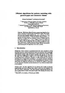
Consider the scenario of Fig. 1, where two cameras C1 and C2 (or, equivalently, the same camera in two different positions) capture two different views of the
212
J.F.C. Mota and P.M.Q. Aguiar
world. As usual when recovering SfM, we assume that a set of N feature points was extracted from each of the images, and their coordinates in the image plane are represented by � � � � (1) (1) (1) (2) (2) (2) x1 x2 · · · xN x1 x2 · · · xN I1 := (1) (1) I2 := (2) (2) (1) (1) , (2) , y1 y2 · · · yN y1 y2 · · · yN where the superscript (i) indexes the points to Ci , for i = 1, 2. Each feature point has 3D coordinates (Xn , Yn , Zn ), with respect to some fixed coordinate frame. Let that frame be attached to C1 such that: 1) the axes X and Y are parallel to the axes x and y of the camera frame; 2) the optical center of the camera C1 is aligned with the axis Z (see Fig. 1). The major challenge when attempting to recover {(Xn , Yn , Zn ), n = 1, . . . , N } from I1 and I2 is the correspondence problem. In fact, we do not know the pairwise correspondences between the columns of I1 and I2 in (1) because there is not a “natural” way to automatically order the feature point projections. Although estimating this ordering leads to a combinatorial problem whose solution, in general, becomes a quagmire for large N , we show in this paper that, when the relative orientation of the cameras is known and the perspective projection is well approximated by the orthographic projection model, an efficient solution can be found. Consider the orthographic model of a camera [1]: x = P X, where X ∈ P3 and x ∈ P2 are, respectively, the homogeneous coordinates of the points in space and in the image plane. The matrix P ∈ R3×4 is given by � � R t P = T , (2) 03 1 where R ∈ R2×3 contains the first two rows of a 3D rotation matrix, t ∈ R2 is a translation vector and 03 is the zero vector in R3 . With the choice of reference
C2 x C1
z
y
Fig. 1. Our scenario, with a choice for the reference frame
Efficient Methods for Point Matching with Known Camera Orientation
213
frame of the previous paragraph, it is straightforward to see that camera C1 (1) (1) captures the first two coordinates of the feature points, i.e., that (xn , yn ) = (Xn , Yn ), n = 1, . . . , N . Naturally, camera C2 captures projections that depend on the relative position of the cameras, the 3D coordinates of the points, and their correspondences: ⎡ ⎤ � � � � X1 X2 · · · XN ⎥ I2 R t ⎢ ⎢ Y1 Y2 · · · YN ⎥ Π, = T (3) 1TN 0 3 1 ⎣ Z1 Z2 · · · ZN ⎦ 1 1 ··· 1 where 1N ∈ RN has all its entries equal to 1, and Π ∈ RN ×N is a permutation matrix, i.e., a matrix with exactly one entry equal to 1 per row and per column and the remaining entries equal to 0 (when we multiply a matrix M by Π, we get a matrix with the same entries of M but with the columns arranged in a possibly different order). By using (3), we obtain the model relating the projections of the feature points in images I1 and I2 with all the unknowns:
ˆ 1 + rˆZ T + t1T Π, I2 = RI (4) N ˆ rˆ], with R ˆ ∈ where Z = [Z1 , Z2 , . . . , ZN ]T and R was decomposed as R = [R, 2×2 2×1 R and rˆ ∈ R . When the relative orientation of the cameras is known (which, as discussed in the previous section, occurs in several practical situaˆ and rˆ are known, the problem becomes to find a permutation tions), i.e., when R matrix Π, a set of 3D point depths {Z1 , . . . , ZN }, and a translation vector t that solve (4). In general, the problem is hard due to the huge cardinality of the set of all N × N permutation matrices: N !.
3
Closed-form Solution for Translation
The choice of the reference frame in the previous section leaves one degree of freedom: we can place the frame at any point along the axis Z. We now choose position in such a way that the problem is simplified: let it be such �this N that n=1 Zn = 1TN Z = 0, i.e., that the plane XY contains the center of mass of the feature points. Multiplying both sides of (4) by 1N and simplifying, we get
ˆ 1 + rˆZ T + t1TN 1N (5) I2 1N = RI ˆ 1 1N + N t. = RI
(6)
where (5) uses the fact that Π 1N = 1N (permutation of a vector with all equal entries) and (6) uses equalities Z T 1N = 0 (from the choice of reference frame)
214
J.F.C. Mota and P.M.Q. Aguiar
and 1TN 1N = N . From (6), we see that the solution for the translation vector t does not depend on the remaining unknowns (Π, Z): � 1 � ˆ 1 1N . I2 − RI (7) t= N By removing the (now known) translation from the problem, i.e., by replacing the solution (7) in (4) (and using 1TN Π = 1TN ), we get
� � ˆ 1 + rˆZ T Π + 1 I2 − RI ˆ 1 1N 1T . (8) I2 = RI N N To simplify notation, we re-define our observations by introducing matrices I˜1 and I˜2 , both computed from known data: � 1 � ˆ 1 1N 1T , ˆ 1. I˜2 := I2 − I2 − RI I˜1 := RI (9) N N With these definitions, problem (4) is re-written as
I˜2 = I˜1 + rˆZ T Π,
(10)
where the unknowns are the depths Z1 , . . . , ZN , in Z, and the correspondences, coded by Π.
4
Optimal Solution for Noiseless Data
We first present an efficient algorithm to compute the solution to our problem when there is no noise, meaning that there exists at least one pair (Z, Π) that solves (10). Naturally, the solution for the permutation matrix Π is given by the association of each column of I˜1 with a column of I˜2 , for the correct value of Z. ˜ n , Y˜n ]T (resp. [˜ Let column n of I˜1 (resp. I˜2 ) be represented by [X xn , y˜n ]T ) and consider the error Eij of associating column j of I˜1 with column i of I˜2 , i.e.,
2
2 ˜ j − rˆ1 Zj + y˜i − Y˜j − rˆ2 Zj , Eij = min x ˜i − X (11) Zj
where rˆ = [ˆ r1 , rˆ2 ]T . The minimizer Zj∗ solving (11) is straightforwardly obtained in closed-form: ˜ j ) + rˆ2 (˜ rˆ1 (˜ xi − X yi − Y˜j ) Zj∗ = . (12) �ˆ r �2 Our algorithm, detailed and analyzed in the sequel, computes for each column i of I˜2 , the column j ∗ of I˜1 that minimizes error Eij (11) with respect to j (without noise, for each i there exists at least one j ∗ such that Eij ∗ = 0). In the algorithm description below, the N × N permutation matrix Π is simply parameterized by a N × 1 vector perm: the jth column of Π has entry permj equal to 1 (and, obviously, the others equal to zero); also, |S| denotes the cardinality of set S and S1 \S2 the set of elements of S1 that do not belong to S2 .
Efficient Methods for Point Matching with Known Camera Orientation
215
Algorithm 1 Inputs Matrices I˜1 and I˜2 , organized into the �corresponding sets of columns � ˜ 1 , Y˜1 ]T , . . . , [X ˜ N , Y˜N ]T } and A = [˜ x1 , y˜1 ]T , . . . , [˜ xN , y˜N ]T , and B1 = {[X vector rˆ. Procedure For i = 1, . . . , N (N = |A|) – For all j = 1, . . . , |Bi |, compute Zj∗ (12) and Eij (11); – j ∗ = arg minj Eij ; – permj ∗ = i, Zj ∗ = Zj∗∗ ; ˜ j ∗ , Y˜j ∗ ]T . – Bi+1 = Bi \[X Outputs Vectors perm and Z. Algorithm 1 consists of N loops where, in each loop, a column of I˜2 is assigned to a column of I˜1 . Each assignment requires a search over, at most, N possibilities. It is then clear that our algorithm has complexity of O(N 2 ), in particular, we obtain the total number of floating point operations (flops) as 7N 2 + 7N − 14. Before proving optimality of Algorithm 1, we interpret it in a geometric way. ˜ j , y˜i − Y˜j ]T , the xi − X Defining each possible “displacement” I˜1 → I˜2 as aij := [˜ 2 cost minimized in (11) can be written as �aij −Zj rˆ� . So, for each column [˜ xi , y˜i ]T T ˜ j , Y˜j ] of I˜1 that minimizes �aij − of I˜2 , our algorithm searches the column [X Zj rˆ�2 for all possible values of Zj . Since this expression achieves its minimum r), (zero) when aij is collinear with rˆ (which we synthetically denote by aij //ˆ Algorithm 1 assigns pairs of columns such that their difference is “as parallel as possible” to rˆ. This collinearity is a re-statement of the fact that epipolar lines are parallel in an orthographic stereo pair [1] (more generally, the trajectories of image projections of a rigid scene can be represented in a rank 1 matrix [5]). Theorem 1 (Optimality of Algorithm 1). If there exists at least one pair (Z, Π), such that (10) holds, then the outputs of Algorithm 1 determine a pair ¯ Π) ¯ that solves (10). (Z, Proof. Suppose the pair (Z ∗ , Π ∗ ) is such that (10) holds. For each i = 1, . . . , N , there exists one and only one k such that ∗ Πki =1
(13)
(because Π ∗ is a permutation matrix). We now denote by j ∗ (i) the assignment produced by Algorithm 1, i.e., we make explicit the dependence of j ∗ on i. Obviously, if j ∗ (i) = k for all i = 1, . . . , N , then the algorithm returned an optimal solution. So, for the remaining of the proof, we assume there is an index i such that j ∗ (i) �= k. We will see that, even in this case, (10) holds for the solution provided by the algorithm, because Eij ∗ (i) = 0, for all i. A simple way to complete the proof is using contradiction. Assume i is the smallest index such that Eij ∗ (i) > 0 (obviously j ∗ (i) �= k). If Eij ∗ (i) > 0, then ˜ k , Y˜k ]T �∈ Bi (at the ith loop). Thus, there exists an index l (1 ≤ l < i) such [X ˜ k , Y˜k ]T (because Elj ∗ (l) = 0 for all 1 ≤ l < i). According to the that [˜ xl , y˜l ]T //[X ˜ k , Y˜k ]T //[˜ xi , y˜i ]T , thus [˜ xl , y˜l ]T //[˜ xi , y˜i ]T . assignment defined by (13), we have [X
216
J.F.C. Mota and P.M.Q. Aguiar
Also, since Π ∗ is a permutation matrix, there exists an index m (1 ≤ m ≤ ∗ ˜ m , Y˜m ]T //[˜ N ), such that Πml = 1, or, equivalently, such that [X xl , y˜l ]T , thus, T T T ˜ ˜ ˜ ˜ xi , y˜i ] . We now consider two cases: 1) if [Xm , Ym ] ∈ Bi , there is [Xm , Ym ] //[˜ ˜ m , Y˜m ]T �∈ Bi , it is straightforward to a contradiction because Eim = 0; 2) if [X T ˜ ˜ ˜ m� , Y˜m� ]T //[˜ find a vector [Xm� , Ym� ] ∈ Bi such that [X xi , y˜i ]T , by performing steps like the ones above, which brings us back to case 1).
5
Approximate Solution for Noisy Data
In practice, not only the knowledge of the camera orientation is uncertain but also the feature point projections are noisy. Since Algorithm 1 is based on the collinearity of a vector that depends on the camera orientation (ˆ r ) with vectors ˜ j , y˜i − Y˜j ]T ), its behavior is that depend on the feature point projections ([˜ xi − X sensitive to disturbances affecting these vectors. We now propose a modification of this algorithm, which results robust not only to the noise but also to violations of the orthographic projection model. From model (10) we note that the clouds of points in I˜1 and I˜2 differ by rˆZ T . Since rˆ contains entries of a rotation matrix, thus with magnitude smaller than 1, in practice, the patterns of points in I˜1 and I˜2 will almost coincide when the depth of the scene is not too large (more rigorously, when rˆZ T is negligible if compared to the minimum distance between points), even if the corresponding points in I1 and I2 are very distant (see an insightful example in Fig. 4). This motivated us to use the matching criterion of minimizing the Euclidean distance between points in I˜1 and I˜2 , � Eij
�� � � ��2 ˜j � � x ˜i X � =� � y˜i − Y˜j � ,
(14)
rather than the less robust collinearity implicit in (11). Algorithm 2 Inputs Matrices I˜1 and I˜2 , organized into the �corresponding sets of columns � ˜ 1 , Y˜1 ]T , . . . , [X ˜ N , Y˜N ]T } and A = [˜ B1 = {[X x1 , y˜1 ]T , . . . , [˜ xN , y˜N ]T , and vector rˆ. Procedure For i = 1, . . . , N (N = |A|) � (14); – For all j = 1, . . . , |Bi |, compute Eij ∗ � – j = arg minj Eij ; – permj ∗ = i, Zj ∗ = Zj∗∗ (12); ˜ j ∗ , Y˜j ∗ ]T . – Bi+1 = Bi \[X Outputs Vectors perm and Z. Our experiments, some of them singled out in the following section, demonstrate that Algorithm 2 successfully infers correct feature point correspondences when dealing with real images. In spite of correctly determining correspondences, the accuracy of the depth estimates in Z strongly depends on the magnitude of the
Efficient Methods for Point Matching with Known Camera Orientation
217
components of rˆ. In fact, assuming the correspondences are known, for example, Π = IN ×N (for simplicity), model (10) becomes I˜2 − I˜1 = rˆZ T , making clear that the accuracy in the estimation of Z depends not only on the accuracy of the measurements (I˜1 , I˜2 , rˆ) but also on the magnitude of the components of rˆ. In particular, we obtain an upper-bound for the depth estimation error as ρZ = max |I˜2 − I˜1 |/ min |ˆ r |. Naturally, when the ratio ρZ is large, we can still use our algorithm to estimate the correspondences between the feature points (the bottleneck of the problem), whose accuracy is not affected by ρZ , and then use a standard algorithm to recover SfM, eventually using a larger set of images to reduce ambiguity, see, e.g., [1].
6
Experiments
To test the algorithms with ground truth, we synthesized data. In particular, we generated the 3D world as a set of 50 points randomly distributed in [−200, 200]3 and relative orientations between the cameras by specifying random rotation matrices. Then, we synthesized measurements according to the model in expression (3), for random permutation matrices. As expected, according to our theoretical derivation of Section 4, Algorithm 1 always produced the correct result: it successfully recovered the permutation, i.e., the correct correspondences between the points, and their depth. To test robustness to disturbances, we then ran experiments by considering inaccurate knowledge of camera orientation and noisy feature point projections. As anticipated in Section 5, we observed that Algorithm 2 results more robust than Algorithm 1. The plot in Fig. 2 illustrates this point by showing the average number of wrong correspondences as functions of the (white Gaussian) measurement noise standard deviation (st.dv.). Note that, even for noise st.dv. of 5 pixels, Algorithm 2 almost always recovers totally correct correspondences. In what respects to depth estimation accuracy, the magnitudes of the errors were smaller than the magnitudes of the measurement noise. We tested our algorithms with real images. Two examples are shown in Fig. 3, which contains the two pairs of images with feature points superimposed. Note that, in both examples, corresponding features are far from being close to each other, preventing thus the usage of “local” methods. We used standard calibration techniques to compute camera orientation [6] and then run our algorithms. The plots in Fig. 4 provide insight over our approach: while the feature point projections of corresponding features in I1 and I2 are in general far apart, their “versions” in I˜1 and I˜2 are close. As a consequence, Algorithm 2 recovered the correct correspondences in both cases. We emphasize that these examples strongly depart from the assumed orthographic projection (see the perspective effects between the pairs of images in Fig. 3), thus, that our approach is able to deal with a wide range of real life scenarios.
218
J.F.C. Mota and P.M.Q. Aguiar
Fig. 2. Number of incorrect correspondences, for a 3D world of 50 points, as functions of the noise power (mean over 1000 runs)
1
15
15
14
6
7
9
8
9 2
3
20
8
14 7
4
6
5 10
11
12
13
17
19
13 12
18 16
18
20 1
11
19
10 3 2 5 17
4 16
11
13
14 2 1
11
12
14 1
4 3
12
2 3
13
4
10 5
9
7 6
8
10
5 6
7
9 8
Fig. 3. Two pairs of real images with feature points superimposed
Efficient Methods for Point Matching with Known Camera Orientation
219
Fig. 4. Left: feature point coordinates in I1 and I2 , extracted from the pair of images in the top of Fig. 3 (the blue circles are from the left image and the red crosses from the right one). Right: corresponding entries of I˜1 and I˜2 , computed from known data, see (9).
7
Conclusion
We proposed efficient algorithms for finding simultaneously the correspondences between points in two images and their depth in the 3D world. Our approach is based on the facts that, in many situations, the relative orientation of the cameras is available, or can be easily inferred, and the camera model can be approximated by an orthographic projection. The resulting complexity is O(N 2 ), where N is the number of feature points (compare with N !, the number of possible correspondences). We prove the optimality of a first algorithm when dealing with noiseless data and develop a modified version that results more robust to uncertainty in the measurements.
References 1. Hartley, R., Zisserman, A.: Multiple View Geometry In Computer Vision. Cambridge University Press, Cambridge (2003) 2. Dellaert, F., Seitz, S., Thorpe, C., Thrun, S.: Structure from motion without correspondence. In: IEEE Conf. on Computer Vision and Pattern Recognition, Hilton Head SC, USA (2000) 3. Shivaswamy, P., Jebara, T.: Permutation invariant SVMs. In: Int. Conf. on Machine Learning, Pittsburgh PA, USA (2006) 4. Martins, A., Aguiar, P., Figueiredo, M.: Orientation in Manhattan. IEEE Trans. on Pattern Analysis and Machine Intelligence 27(5) (2005) 5. Aguiar, P., Moura, J.: Rank 1 weighted factorization for 3D structure recovery: Algorithms and performance analysis. IEEE Trans. on Pattern Analysis and Machine Intelligence 25(9) (2003) 6. Bouguet, J.: Camera calibration toolbox for Matlab (2008), http://www.vision.caltech.edu/bouguetj/calib_doc