Task Clustering and Gating for Bayesian Multitask Learning

Journal of Machine Learning Research 4 (2003) 83-99

Submitted 8/02; Published 5/03

Task Clustering and Gating for Bayesian Multitask Learning Bart Bakker Tom Heskes

BARTB @ SNN . KUN . NL TOM @ SNN . KUN . NL

SNN, University of Nijmegen Geert Grooteplein 21 6525 EZ Nijmegen, The Netherlands

Editor: Michael I. Jordan

Abstract Modeling a collection of similar regression or classification tasks can be improved by making the tasks ‘learn from each other’. In machine learning, this subject is approached through ‘multitask learning’, where parallel tasks are modeled as multiple outputs of the same network. In multilevel analysis this is generally implemented through the mixed-effects linear model where a distinction is made between ‘fixed effects’, which are the same for all tasks, and ‘random effects’, which may vary between tasks. In the present article we will adopt a Bayesian approach in which some of the model parameters are shared (the same for all tasks) and others more loosely connected through a joint prior distribution that can be learned from the data. We seek in this way to combine the best parts of both the statistical multilevel approach and the neural network machinery. The standard assumption expressed in both approaches is that each task can learn equally well from any other task. In this article we extend the model by allowing more differentiation in the similarities between tasks. One such extension is to make the prior mean depend on higher-level task characteristics. More unsupervised clustering of tasks is obtained if we go from a single Gaussian prior to a mixture of Gaussians. This can be further generalized to a mixture of experts architecture with the gates depending on task characteristics. All three extensions are demonstrated through application both on an artificial data set and on two realworld problems, one a school problem and the other involving single-copy newspaper sales. Keywords: Empirical Bayes; Multitask learning; Mixture of experts; Multilevel analysis.

1. Introduction Many real-world problems can be seen as a series of similar, yet self contained tasks. Examples are the school problems (see e.g. Aitkin and Longford, 1986), and clinical trials. The first example deals with the prediction of student test results for a collection of schools, based on school demographics. The similar tasks in the other example can be the prediction of survival of patients in different clinics (see e.g. Daniels and Gatsonis, 1999). The relatedness (and therefore interdependency) of such models is taken into account and benefitted from in the fields of multitask learning (or learning to learn) and ‘multilevel analysis’. In the present article we seek to combine insights that are obtained in the multilevel field with methods that have been designed in the neural network community to create a synergetic new approach. Multilevel analysis is generally based on the ‘mixed-effects linear model’. This model features a response that is made up from the sum of a fixed effect and a random effect. The fixed effect implements a ‘hard sharing’ of parameters, whereas the random effect implies a ‘soft sharing’ through the use of a common distribution for certain model parameters. A more elaborate description of multilevel analysis is given in Section 6. A neural network model would use ‘hard shared’ parameters (the same for each of the parallel tasks) to detect ‘features’ in the covariates x, and use these features for regression (Baxter, 1997, Caruana, 1997). Feature detection can be implemented, for example, in the hidden layers of a multi-layered perceptron, or through principal component analysis. This use of features is appropriate when the covariates are relatively high-dimensional, as they are for the real-world problems addressed in the present article. In our approach, all shared parameters, including but not restricted to the hyperparameters specifying the prior, are inferred through a maximum likelihood procedure: they are ‘learned’ from the data. This type of

c

2003 Bart Bakker and Tom Heskes.

BAKKER AND H ESKES

outputs yµi

Ai

hµik

bias

W

inputs xµij

bias

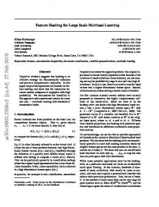
Figure 1: Neural network model. The input-to-hidden weights W are shared by (equal for) all tasks. Each of the outputs (top layer) represents one task, and has its own set of task-dependent hidden-to-output weights Ai .

optimization has previously been studied by Baxter (1997): he showed that the risk of overfitting the shared parameters is an order N (the number of tasks) smaller than overfitting the task-specific parameters (hiddento-output weights). The remaining parameters specific to each task are treated in a Bayesian manner. In the multitask setting, where data from all tasks can be used to fit the shared parameters, this empirical Bayesian approach is a natural choice and a close approximation to a full Bayesian treatment. Any multitask learning model makes use of the fact that the tasks (the parallel sets of responses and covariates) are somehow related. Although for particular sets of tasks the nature of this relationship may be immediately clear, on other occasions more subtle relations may exist. Even if all tasks in a set are related, some may be stronger related to each other than to others. We accommodate for this possibility by suggesting a form of ‘task clustering’ (Section 4). Allowing a fixed number of task clusters we are able to obtain better estimates for the responses y, and discern hidden structure within the set of tasks. We will describe the general structure of the multitask learning model in Section 2. We present our Bayesian treatment of multitask learning and knowledge sharing in Section 3, and show how to optimize the shared parameters of the model. In Section 4 we extend the method so that it may allow a distinction between (groups of) tasks. The model is tested (Section 5) both on an artificial data set, which consists of samples drawn from a mixture of Gaussians, and on two real-world data sets: the Junior School Problem (predicting test results for British school children) and the Telegraaf problem (predicting newspaper sales in The Netherlands). We show that the method presented in this article yields both better predictions and a meaningful clustering of the data. Section 6 describes the links of the present article with related work. We finish with concluding remarks and an outlook on future work in Section 7.

2. A Neural Network Model µ

µ

Suppose that for task i we are given a data set Di = {xi , yi }, with µ = 1 . . . ni , the number of examples for task i. For notational convenience, we assume that the response yµi is one-dimensional. The input xµi is an µ µ ninput -dimensional vector with components xik . Our model assumption is that the response yi is the output of a multi-layered perceptron with additional Gaussian noise of standard deviation σ (see also Figure 1). Each output unit represents the response for one task. Throughout the article we will use networks with one layer of hidden units, with either linear or nonlinear (tanh) transfer functions, and bias. The transfer functions on the outputs will be linear. The bottom layer of this network creates that lower-dimensional representation (see e.g. Baxter, 1997) of the inputs, that is best suited for the second layer to perform regression on.

84

TASK C LUSTERING FOR M ULTITASK L EARNING

In our model, the input-to-hidden weights W are shared by (equal for) all tasks, whereas the hidden-toµ output weights are task-dependent (see Figure 1). In this format the expression for the response yi reads: ! n nhidden

µ

yi =

∑

µ

µ

Ai j hi j + Ai0 + noise , hi j = g

j=1

input

∑

µ

W jk xik + W j0

,

(1)

k=1

with W the nhidden × (ninput + 1) matrix of input-to-hidden weights (including bias) and Ai an (nhidden + 1)µ dimensional vector of hidden-to-output weights (and bias). The extra index i in the hidden unit activity hi µ µ follows from the dependency of the covariates xi on task i. For notational simplicity we will include hi0 = 1 µ in hi and Ai0 in Ai from now on.

3. Computation and Optimization Let us now consider the full set of tasks, for which we define the complete data set D = {Di }, with i = 1 . . . N, µ the number of tasks. For notational convenience we will assume all inputs xi fixed and given and omit them from our notation. A denotes the full N × (nhidden + 1)-dimensional matrix of hidden-to-output weights. Note that these are specific for each task, whereas all other parameters are shared between tasks. We assume the tasks to be iid given the hyperparameters, and define a prior distribution for the task-dependent parameters: Ai ∼ N (Ai |m, Σ) ,

(2)

which is a Gaussian with an (nhidden + 1)-dimensional mean m and an (nhidden + 1) × (nhidden + 1) covariance matrix Σ. This prior distribution is incorporated into the posterior probability of data and hidden-to-output weights given the hyperparameters Λ = {W, m, Σ, σ}. The joint distribution of data and model parameters reads N

P(D, A|Λ) = ∏ P(Di |Ai ,W, σ)P(Ai |m, Σ) , i=1

where we used the assumption that the tasks are iid given Λ. Integrating over A we obtain, after some calculations (see Appendix A for details) N

P(D|Λ) = ∏ P(Di |Λ) , i=1

with

 − 1   2 1 2ni P(Di |Λ) ∝ |Σ|σ |Qi | exp (RTi Q−1 R − S ) , i i i 2

(3)

where Qi , Ri and Si are functions of Di and Λ given by Qi Si

= =

ni

∑ hi hi + Σ−1 , Ri = σ−2

σ−2 σ−2

µ=1 ni

µ µT

∑ yµi

2

+ mT Σ−1 m .

ni

∑ yi hi + Σ−1m , µ µ

µ=1

(4)

µ=1 µ

µ

(Recall that hi depends on W and xi .) Optimal parameters Λ∗ are now computed by maximizing the likelihood (3). This is referred to as empirical Bayes (Robert, 1994), and is similar to MacKay’s evidence framework (MacKay, 1995). Here it is motivated by the fact that we can use the data of all tasks to optimize Λ, the dimension of which is independent of and assumed to be much smaller than the number of tasks. In the limit of infinite tasks the empirical Bayesian approach coincides with the full Bayesian approach. For finite 85

BAKKER AND H ESKES

numbers of tasks, Baxter (1997) shows that the generalization error as a function of the number of tasks N and the dimension of the hyperparameters |Λ| is proportional to |Λ| and inversely proportional to N (see also Heskes, 2000). Given the maximum likelihood parameters Λ∗ , we can easily compute P(Ai |Di , Λ∗ ) to make predictions, compute error bars, and so on. The parameter ˜ i = argmax P(Ai |Di , Λ∗ ) A Ai

will be referred to as the maximum a posteriori or MAP value for Ai . When g(·) in (1) is a linear function, we can simplify Equation 3 significantly (see Appendix A). This µ µ gives us the advantage the full data sets Di = {xi , yi } for each task, we only need the

Tthat  instead of using  sufficient statistics xi xi , hxi yi i and y2i for optimization, where h..i denotes the average over all examples µ.

4. Making Some Tasks More Similar Than Others The prior (2) may be useful when we have reason to believe that a priori all tasks are ‘equally similar’. In many applications, this assumption is a little too simplistic and we have to consider more sophisticated priors. 4.1 Task-dependent Prior Mean We can make the prior distribution task-dependent by introducing higher-level task characteristics, that is, ‘features’ of the task that are known beforehand. We will denote them fi for task i. These features, although they have different values for different tasks, do not vary within one task. Therefore, rather than adding them as extra inputs, we use these features to make the prior mean task-dependent. A straightforward way to include these features into the prior mean is to make it a linear function of these features, that is, mi = Mfi , with M now an (nhidden + 1) × nfeature matrix. We are back to the independent prior mean if we take nfeature = 1 and all fi = 1. The calculation of the likelihood proceeds as in Section 3, with m in (4) replaced by mi . With a linear form optimization is hardly more involved, but in principle we can take more complicated nonlinear dependencies into account as well. 4.2 Clustering of Tasks Another reasonable assumption might be that we have several clusters of similar tasks instead of a single cluster. Then we could take as a prior a mixture of ncluster Gaussians, ncluster

Ai ∼

∑

α=1

qα N (mα , Σα )

(5)

instead of the single Gaussian (2). Each Gaussian in this mixture can be seen to describe one ‘cluster’ of tasks. In Equation 5, qα represents the a priori probability for any task to be ‘assigned to’ cluster α (see also Figure 2). Although a priori we still do not distinguish between different tasks, a posteriori tasks can be assigned to different clusters. The posterior data likelihood reads: P(Di |Λ) =

Z

dAi P(Di |Ai , Λ)

ncluster

∑

α=1

qα P(Ai |mα , Σα ) .

(6)

The major ‘probability mass’ of this integral lies in areas where the parameters Ai both lead to high probabilities of the data (are able to fit the data well) and have high probability under P(Ai |mα , Σα ) themselves. In 86

TASK C LUSTERING FOR M ULTITASK L EARNING

P1 (A | m 1 , Σ 1)

q 11

q2

q1 µ

f1 µ

y1

P2 (A | m 2 , Σ 2)

P1 (A | m 1 , Σ 1)

P2 (A | m 2 , Σ 2)

yn

q n2 q n1

q 12 µ

µ

y1

y2

µ

y3

fn

µ

yn

Ai

Ai µ

h ik

µ

h ik

bias

inputs x µij

bias

inputs x µij

bias

bias

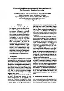
Figure 2: The task clustering (left) and task gating model (right). In task clustering the task-dependent weights Ai are supposed to be drawn from a weighted sum of Gaussians, where the weights qα are equal for all tasks. In task gating these weights become task-dependent and the value for qiα depends on the task-specific feature vector fi .

this way, the posterior distribution effectively ‘assigns’ tasks to that cluster that is most compatible with the data within the task, in the sense that all other clusters (Gaussians) do contribute much less to (6). We introduce indicator variables ziα where ziα equals one if task i is assigned to cluster α and zero otherwise. For any task i only one ziα may be one. To optimize the likelihood of the shared parameters Λ, which now include all cluster means and covariances as well as the prior assignment probabilities q, we can apply an expectation-maximization or EM-algorithm (see e.g. Dempster et al., 1977). If the cluster assignments ziα were known, optimization of log P(D, z|Λ) with respect to Λ would be relatively simple. The values for ziα however are not known, so in the E-step we estimate the expectation value of log P(D, z|Λ) under P(z|D, Λn ), where for Λn we take the current values for Λ (which are initialized randomly at the start of the procedure). In the M-step the obtained expectation value is maximized for Λ. This step is of roughly the same complexity as the optimization for a single cluster. Both steps are repeated until Λ converges to a (local) optimum. This implementation of the EM algorithm is described in more detail in Appendix B. 4.3 Gating of Tasks A possible disadvantage of the above task clustering approach is that the prior is task-independent: a priori all tasks are assigned to each of the clusters with the same probabilities qα . A natural extension is to incorporate the task-dependent features fi that were introduced in 4.1 in a gating model (see Figure 2), for example by defining T T qiα = eUα fi / ∑ eUα′ fi , α′

with Uα an nfeature -dimensional vector. The a priori assignment probability of task i to cluster α is now taskdependent. Uα performs a similar function as the matrix M in Section 4.1: for each task, it translates the task-dependent feature vector fi to a preference for one or more of the clusters α. Uα is added to the set of hyperparameters Λ and learned from the data. The above task clustering approach is a special case with nfeature = 1 and fi = 1 for all tasks i. The EM algorithm is similar to the one described in Appendix B: we simply replace qα with qiα . The M-step for the parameters Uα becomes slightly more complicated, and can be solved using an iterative reweighted least-squares (IRLS) algorithm. The task gating part of our model can be compared to the mixture of experts

87

BAKKER AND H ESKES

model (Jordan and Jacobs, 1994). An important difference is that we use a separate set of higher-level features to gate tasks rather than individual inputs.

5. Results We tested our method on three databases, which are described in the following paragraphs. We implemented neural networks that feature two hidden units with hyperbolic tangents as transfer functions, and linear output units. Networks with more (or less) hidden units did not significantly improve prediction. Each hidden and each output unit contains an additive bias (see also Figure 1). For each dataset we also consider the performance of the single task learning method (training a separate neural network for each task). For the school and the newspaper data, we also look at non-Bayesian multitask learning: in this intermediate model we applied the same network structure as in the Bayesian multitask learning model, yet instead of estimating a prior distribution we learned all model parameters directly. For these two non-Bayesian methods we applied early stopping (see e.g. Caruana et al., 2001) to prevent overfitting on the training data (the model parameters were optimized on a training set, and the optimization process stopped when no more improvement was found on a separate validation set). All algorithms were implemented in MATLAB, and can be downloaded from the authors’ website (http://www.snn.kun.nl/˜bartb/) or from http://www.jmlr.org. 5.1 Description of the Data Artificial Data. We created a data set of artificial data, by drawing random covariates xµi and shared paµ rameters Λ (see Appendix C for the exact values.). The xi were scaled per task to have zero mean and unit µ variance. The responses yi were drawn according to (1), where we used a generative model with one hidden unit and two clusters (two choices for mα ). The artificial data did not include task-dependent features fi . We studied both data sets for g(x) = tanh(x), and g(x) = x. To test our methods we ran 10 independent simulations, where each time we used a random selection of 10 covariates and their corresponding responses per task for optimization, and a large independent test set (300 samples per task) to check the performance of the model. In each simulation, we used 250 parallel tasks. School Data. This data set, made available by the Inner London Education Authority (ILEA), consists of examination records from 139 secondary schools in years 1985, 1986 and 1987. It is a random 50% sample with 15362 students. The data set has been used to study the effectiveness of schools. A file containing the database can be downloaded from the ‘Multilevel Page’ (http://multilevel.ioe.ac.uk/intro/datasets.html). See also Mortimore et al. (1988). Each task in this setting is to predict exam scores for students in one school, based on eight inputs. The first four inputs (year of the exam, gender, VR band and ethnic group) are student-dependent, the next four (percentage of students eligible for free school meals, percentage of students in VR band one, school gender (mixed or (fe)male only) and school denomination) are school-dependent. The categorical variables (year, ethnic group and school denomination) were split up in binary variables, one for each category, making a new total of 16 student-dependent inputs, and six school-dependent inputs. We scaled each covariate and output to have zero mean and unit variance. All performance measures are obtained after making 10 independent random splits of each school’s data (covariates and corresponding responses) into a ‘training set’ (containing on average 80 samples), used both for fitting the shared parameters and computing the MAP hidden-to-output weights, and a ‘test set’ (comprised of the remaining samples, 30 on average) for assessing the generalization performance. Prediction of Newspaper Sales. We also applied our methods on a database of single-copy sales figures for one of the major Dutch newspapers. The database contains the numbers of newspapers sold on 156 consecutive Saturdays, at 343 outlets in The Netherlands. Inputs include recent sales (four to six weeks in the past), last year’s sales (51 to 53 weeks in the past), weather information (temperature, wind, sunshine, precipitation quantity and duration) and season (cosine and sine of scaled week number). The responses are the realized sales figures. Considering a single task, our model can be interpreted as an auto-regressive model

88

TASK C LUSTERING FOR M ULTITASK L EARNING

Table 1: Explained variance for each of the combinations of model and database.

linear model on linear data linear model on nonlinear data nonlinear model on linear data nonlinear model on nonlinear data

single cluster 40.5 ± 0.5 % 22.0 ± 0.3 % 40.9 ± 0.4 % 23.3 ± 0.5 %

task clustering 43.3 ± 0.5 % 23.8 ± 0.9 % 40.9 ± 0.5 % 24.9 ± 0.6 %

with additional covariates. All covariates and responses were scaled per task (outlet) to zero mean and unit variance. Performance measures were obtained as for the school data, where now the ‘training set’ contains 100 samples per task and the ‘test set’ contains the remaining 56 samples. For the task-dependent mean and the gating of tasks we constructed two features depending on the outlet’s location: the first feature codes the number of local inhabitants (from zero, less than 15,000, to four, more than 300,000), the second one the level of tourism (from zero, hardly any tourism, to two, very touristic). 5.2 Generalization Performance Artificial Data. We applied both the linear and the nonlinear method to the two databases we created, resulting in four combinations. In each of these four combinations we applied both the multitask learning method with one cluster, and model clustering. As can be seen in Figure 3, in all four cases the method was able to discern the two clusters. Note that in the second panel (linear model working on nonlinear data) one of the priors is ‘flattened’, indicating that in this case only part of the (nonlinear) structure could be found. Table 1 presents a model evaluation in terms of the percentage of variance explained by both models with and without clustering. Percentage explained variance is defined as the total variance of the data minus the sum-squared error on the test set as a percentage of the total data variance. All combinations of model and database except the nonlinear model on the linear database showed significant improvements when task clustering is implemented. Note also that nonlinear multitask learning on the linear database performed equally well as the linear method. Apart from this, the nonlinear model worked best for the nonlinear database and the linear model for the linear database. For both databases, single task learning explained less than one percent of the variance. School Data. We applied single task learning, non-Bayesian and Bayesian multitask learning on the school data. The results are expressed in Table 2. Single task learning explained 9.7% of the variance, which was much less than any of the multitask learning methods. Non-Bayesian multitask learning explained 29.2% of the variance. The overall winners were the Bayesian methods with one and two priors (clusters) with an explained variance of 29.5%. Implementation of the methods described in Section 4 yielded no improvement on the ‘single cluster’ multitask learning method. This lack of improvement was also reflected in the clusters obtained: either two very similar priors were created, or one cluster was found to contain all tasks, whereas the other was empty. Although task clustering did not yield a significant improvement here, at least the results show that the method does not force structure on the data where there is no structure present. Prediction of Newspaper Sales. The model of Section 2 (single Gaussian prior) managed to explain 11.1% of the variance in the test data, much better than the 9.0% explained variance with the same multitask model regularized through early stopping instead of through a ‘learned’ prior. Note that this regression problem has a very low signal-to-noise ratio, also due to the fact that, for a fair real-world comparison, only sales figures from at least four weeks ago can be used as covariates. When all tasks were optimized independently using all 13 covariates, less than one percent explained variance was achieved. These results are consistent with the more extended simulation studies in (Heskes, 1998, 2000). The more involved methods of Section 4 all led to a slightly, but significantly better performance, explaining another 0.1% of the variance. Although not spectacular, translated to the set of more than 10,000 Dutch outlets for which predictions have to be made on a daily basis, this might still be worthwhile.

89

BAKKER AND H ESKES

linear on linear

linear on nonlinear 10

0

ML

ML

5

0

−5 −10

−5

−10 −100 5

0

−50

0

50

100

MAP

MAP

5 0

0

−5 −10

−5

−5 −5

0

nonlinear on linear

10

15

20

5 ML

ML

5

nonlinear on nonlinear

5 0 −5 −60

0

0 −5

−40

−20

0

20

−15 5

−10

−5

0

5

MAP

MAP

5 0

0

−5 −60

−40

−20

0

−5 −6

20

−4

−2

0

2

Figure 3: Maximum likelihood (upper panels, marked ML) and maximum a posteriori (lower panels, marked MAP) values for the model parameters Ai in the artificial data paradigm. Each dot or diamond refers to one task, where (in the lower panels) identical marks (dots or diamonds) indicate tasks that belong to the same cluster (are generated around the same mean). In each panel, the horizontal axis corresponds to the hidden-to-output weight, the vertical axis to the bias. The 95% confidence intervals for the two estimated priors are plotted in the lower panels. From left to right and up to down, the panels show the results for the linear model on the linear data, the same model on the nonlinear data, the nonlinear model on the linear data and on the nonlinear data. The means mα used for generation of the data sets (corrected for the difference between the true and estimated hidden unit activity) are depicted by stars in the 8 panels.

Although for each database the more involved methods (such as task clustering or gating) required more computation time than the simpler methods (such as non-Bayesian multitask learning), all times were in the same order of magnitude. None of the simulations took more than 30 minutes (on a Pentium 3). In general, when a method was able to explain a higher percentage of the variance, it also required more computation time. The one exception to this rule was the single task learning method: although it performed (relatively) poorly on all of the databases, it actually required more time than non-Bayesian multitask learning. This is

90

TASK C LUSTERING FOR M ULTITASK L EARNING

Table 2: Explained variance for the school data and the newspaper data. The evaluated methods are single task learning (STL), maximum likelihood multitask learning (ML MTL), Bayesian multitask learning, task clustering with two clusters and task gating with two clusters.

school data newspaper sales

STL 9.7 ± 0.7 %