Efficient Trajectory Joins using Symbolic Representations - CiteSeerX

Efficient Trajectory Joins using Symbolic Representations Petko Bakalov

Marios Hadjieleftheriou

Eamonn Keogh

University of California, Riverside [email protected]

University of California, Riverside [email protected]

University of California, Riverside [email protected]

Vassilis J. Tsotras University of California, Riverside [email protected]

Abstract Efficiently and accurately discovering similarities among moving object trajectories is a difficult problem that appears in many spatiotemporal applications. In this paper we consider how to efficiently evaluate trajectory joins, i.e., how to identify all pairs of similar trajectories between two datasets. Our approach represents an object trajectory as a sequence of symbols (i.e., a string). Based on special lower-bounding distances between two strings, we propose a pruning heuristic for reducing the number of trajectory pairs that need to be examined. Furthermore, we present an indexing scheme designed to support efficient evaluation of string similarities in secondary storage. Through a comprehensive experimental evaluation we present the advantages of the proposed techniques.

1.

Introduction

Moving object representation, storage and processing has received a lot of attention recently [14, 21, 25, 28, 30, 3, 8, 33, 10, 6, 27, 22, 5]. The emergence of affordable GPS devices has enabled easy tracking of moving object trajectories. In combination with cheap storage devices it is nowadays possible to maintain large repositories of such data. This abundance of information motivates the need to develop efficient techniques for answering interesting queries about the past behavior of moving objects. Previous research conducted for historical spatio-temporal data management has mainly focused on algorithms for answering two types of queries, namely range searches and nearest neighbors (and their respective variations). For instance: “Find all airplanes that crossed area A” or “Identify the car that passed the closest from point A”. In this paper we address a novel query, namely the trajectory join, i.e., the problem of identifying all pairs of similar trajectories between two datasets. Such queries can be useThis work was partially supported by NSF grants IIS9907477, EIA-9983445, IIS-0220148.

Permission to make digital or hard copies of all or part of this work for personal or classroom use is granted without fee provided that copies are not made or distributed for profit or commercial advantage and that copies bear this notice and the full citation on the first page. To copy otherwise, to republish, to post on servers or to redistribute to lists, requires prior specific permission and/or a fee. MDM 2005 05 Ayia Napa Cyprus Copyright 2005 ACM 1-59593-041-8/05/05 ...$5.00.

ful in many applications, for example to identify delivery or transportation vehicles that follow similar routes and can thus be eliminated, e.g., “Identify the pairs of trucks that were never apart from each other for more than 1 mile this morning”. Here, we deal with the restricted version of the problem where a temporal predicate is specified by the query (e.g., “this morning”). The general trajectory join query requires expensive evaluation algorithms more relevant to mining applications [29, 30]. By restricting similarity evaluation only inside a user specified time-interval, we render the problem more amenable to solutions that can use specialized index structures for evaluating the joins. For the applications that we target (e.g., the delivery trucks query mentioned before) the temporal dimension has as much significance as the spatial dimensions of the data. Thus, we do not consider data normalization, neither arbitrary time shifts when evaluating similarities. Nevertheless, our techniques could also support small scale time-warping by appropriately choosing the trajectory similarity functions used.

2. Preliminaries 2.1

Related Work

A naive approach for evaluating trajectory joins between two given datasets would be to compare each trajectory contained in the first dataset with all trajectories contained in the second. Clearly, even if the two datasets are stored sequentially on disk, the amount of I/O needed by the naive solution would be prohibitive, especially for large trajectory repositories. Many join and self-join algorithms have been designed specifically for categorical, numerical and spatial data [2, 18, 20, 24, 15, 26, 11, 32, 23, 17, 19, 1, 7]. However, these algorithms are not applicable in the case of spatio-temporal trajectories. Another straightforward solution would be to use a spatio-temporal index structure [14, 10, 25, 28] to evaluate the temporal condition of the join queries first, and then retrieve only the candidate trajectories. A nested loop join algorithm could be used to produce the final answers. In our scenario we assume that the selectivity of the temporal predicate in general will by very low, meaning that a very large number of trajectories will be retrieved as possible candidates (in the worst case where all data trajectories span the complete dataset lifetime, for any given query time-interval all trajectories would need to be retrieved). In this paper we use a specialized trajectory representation and storage that can be exploited by our algorithm in order to reduce the number of trajectory pairs that need to be compared for evaluating the join queries.

Time

ε

δt

Y X Figure 1: The centric shape formed when using radius threshold ².

2.2

Formal Definition

For simplicity assume that a moving object trajectory is defined as a sequence of location/time-instant pairs. In general, any other trajectory representation should be easily reduced to this general form. More formally: Definition 1. A trajectory T is a sequence of pairs {hl1 , t1 i, . . . , hln , tn i}, where li ∈ Rd , ti ∈ N. The trajectory join query can be defined as follows: Definition 2. Given two sets of object trajectories R and S, a threshold ² and time interval δt, the result of the trajectory join query is a subset V of pairs hRi , Sj i (where Ri ∈ R, Sj ∈ S), such that during time-interval δt the distance Dδt (Ri , Sj ) ≤ ², for any pair in V and any user defined distance function D. In other words, for each pair of trajectories in V it holds that one trajectory stays inside the centric shape formed by the other trajectory when extended with radius ² in space for every time-instant in the duration of time-interval δt (see Figure 1). The naive approach for solving this problem will have complexity equal to the size of the Cartesian product R × S. For very large sets R or S, the I/O cost of this approach will be prohibitive in practice. The user defined distance function D (which is used here as an inverse measure of trajectory similarity without loss of correctness) is allowed to be arbitrary in the general definition. Although, for the techniques proposed in this work it will be mandatory to specify distance functions that are metric (i.e., satisfy the triangular inequality) or that can at least be lower-bounded by a distance function that is metric. In practice, all popular distance measures (e.g., the Lp -norm and the Dynamic Time Warping) satisfy this property.

3.

Trajectory Join Evaluation

Motivated by the expensive nature of the naive algorithm we seek solutions for evaluating trajectory joins more efficiently. The fundamental idea is to find a way to prune as many trajectory pair similarity evaluations as possible. Straightforwardly, a specialized index structure can be designed for this purpose. First, we give a brief overview of the proposed solution and then we present our technique in more detail.

Clearly, in order to be able to index the trajectories for the purpose of efficient similarity evaluation we need to introduce a lower-bounding distance function that can be computed efficiently for arbitrary time-intervals between pairs of trajectories, without having to access the complete trajectory information. This can be achieved by storing an approximate representation of the trajectories only for the purpose of computing relevant lower-bounding distances according to the given query time-intervals. Then, a large volume of the exact trajectory representations that do not qualify for threshold ² can be pruned, by referring only to the reduced, approximate dataset. Subsequently, a post filtering step can eliminate the false alarms produced by the approximations. By tuning the approximation accuracy we can adjust the number of false alarms introduced in the intermediate result. The final cost of a single query will comprise of two parts: (1) The cost of computing the lower-bounding distances (dominated by the total size of the approximate data that needs to be loaded from storage) and (2) the cost of executing the filtering step (dominated by the total number of exact data trajectories that need to be retrieved). An ideal solution needs to be able to leverage the lower-bounding distance evaluation cost and the cost of the post filtering step. We argue, and also confirm using a comprehensive experimental evaluation, that for reasonably sized time-interval query predicates a carefully structured approximate trajectory index — one order of magnitude smaller then the total size of the exact trajectory representations — is adequate for improving trajectory join query performance by as much as three orders of magnitude when compared with the naive approach. Hence, the problem is reduced to that of choosing appropriate trajectory approximations with the following properties: (1) Support for lower-bounding measures of a large number of trajectory distance functions; (2) support for varying approximation accuracy according to given space constraints; and (3) amenable to efficient indexing that enables fast computation of the lower-bounding distances. An approximation technique that has the aforementioned properties is the symbolic representation of time-series proposed by Lin et al. [16]. This approach first uses the Piecewise Aggregate Approximation (PAA) [13, 31] and then reduces PAA to strings of symbols from a predefined alphabet. Using this technique we can approximate the trajectories using strings of arbitrary length, according to the desired approximation accuracy. Then, by defining an appropriate distance function for strings and showing that this function is a lowerbounding measure of user defined function D, we will be able to approximately evaluate the trajectory join using only the reduced dataset of strings. Finally, we show how the string approximations can be organized on secondary storage such that the computation of lower-bounding distance functions between trajectory pairs for arbitrary time-intervals can be computed very efficiently by taking advantage of the benefits of sequential I/O.

3.1

Symbolic Representations for Trajectories

As already mentioned, the symbolic representations for time-series proposed by Lin et al. [16] first utilize the Piecewise Aggregate Approximation (PAA) technique introduced in [13, 31] and then transform PAA into a string. For ease of exposition, here we present the basic concepts behind

X α5 α4 α3 α2 α1 Time 5 10 15 20 Figure 2: An object trajectory, its PAA representation, and its string representation α4 α3 α2 α1 α2 .

symbolic representations for 1-dimensional time-series and show that they can be straightforwardly applied for multidimensional trajectories. PAA accepts as input a time-series of length n and produces as output an approximation of reduced size, say m. The algorithm divides the input sequence into m equi-sized “frames” and replaces the values contained in each frame using the average of these values. More formally: Definition 3. Given time-series X = {x1 , . . . , xn } of length n and a target length m ¿ n, PAA produces an ap¯ = {¯ proximate time-series X x1 , . . . , x ¯m } where the values n n (i − 1), m i], 1 ≤ i ≤ m are contained inside each frame [ m replaced by their arithmetic mean: n

m x ¯i = n

i m X

xj

n (i−1)+1 j= m

The advantage of PAA is that the length of the reduced time-series m can be chosen at will, thus the accuracy of the resulting approximation can be tuned freely. As a second step the PAA approximation can be discretized by using a symbolic representation. Lin et al. [16] propose using a discretization of the value domain such that the symbols produced have equal probabilities. Nevertheless, for our purposes and due to the nature of join queries, equiprobable symbols need not be considered. Instead, we chose to discretize the PAA approximations by discretizing the original value domain using a uniform grid and assigning a unique symbol to every partition of the grid. An example is shown in Figure 2. Thus, the alphabet size that we consider depends on the granularity of the chosen grid. The finer the granularity, the larger the alphabet size that needs to be supported, and thus the larger the representation size of each individual symbol. The symbolic representation can formally be defined as follows: Definition 4. Given a uniform grid with granularity τ assign an alphabet of symbols A = {α1 , . . . , αw } such that ∀1 ≤ j ≤ w : [τ (j −1), τ j) → αj (every symbol is assigned to a unique interval of the grid). A time-series X of length n ˜ = h˜ can be approximately represented as a string X x1 · · · x ˜m i of length m ¿ n, by replacing every value x ¯i in the m-length PAA approximation of X with symbol x ˜i = αj such that τ (j − 1) ≤ x ¯i < τ j. The exact same concept can be applied for moving object trajectories in a multi-dimensional space. PAA frames correspond to the temporal dimension of the trajectories, while

the chosen alphabet corresponds to a multi-dimensional spatial partitioning of the data universe into disjoint cells. By adjusting the size of alphabet A we can tune the representation size of the strings in the spatial dimensions (according to space discretization); while by adjusting the size of each frame in PAA we can tune the size of the approximations on the temporal dimension (the length of the strings). Notice that omitting the symbolic discretization step is equivalent to using an alphabet size with an infinite number of symbols (i.e., a discretization fine enough that uses a binary symbol representation that has equal size to the binary representations of the actual trajectory data; e.g., 8 bytes for a double value). In the rest, we will refer to this approximation as the direct symbolic representation.

3.2

Symbolic Distance Measures

Having defined a symbolic representation for trajectories we need to introduce a distance function that appropriately lower-bounds the given trajectory distance function D. Assume in the rest for simplicity that a Euclidean distance function is used: sX (xi − yi )2 Dδt (X, Y ) = i∈δt

In the simple 1-dimensional case it can be proven that the following distance on the symbolic representations is always a lower-bound of the Euclidean distance: r s n X ˜ ˜ ˜ Dδt (X, Y ) = d(˜ xi , y˜i )2 t i∈δt

where i ∈ δt corresponds to all frames completely covered by time-interval δt (i.e., the total number of symbols in the string representation contained in δt), t is the total number of such frames, and distance d between two alphabet symbols will be discussed shortly. The following holds: ˜ δt (X, ˜ Y˜ ) ≤ Dδt (X, Y ), for any given trajecClaim 1. D tory X and Y . A proof appears in [4, 12, 31]. For our purposes it is also important to show that the lower-bounding distance is a metric. The proof is straightforward, but due to lack of space it is omitted. The distance function d(αi , αj ) for the general multi dimensional case can be computed simply as the minimum distance between the two grid cells corresponding to symbols αi and αj , as shown in Figure 3. This guarantees that the distance lower-bounds the actual Euclidean distance between any two points that fall inside the respective cells. For small dimensionality we can use a lookup table to evaluate d fast. For larger dimensionality where the lookup table would become unacceptably large, the minimum distance between two symbols can be computed on the fly (all we need to know is the assignment function of a symbol to a cell). Lower-bounding measures for other distance functions can also be devised similarly. For example, we can easily introduce a time warping factor into the proposed distance measure (for comparing distances between symbols at neighboring time-instants) and still preserve the lower-bounding property from a respective time-warped original distance [29].

Y

X 3

α 25

α 21

2 α 13

1

R1 S R2

0

X Figure 3: Computation of function d(αi , αj ). ~

O

~

S3

S2 ~

R2

~ ~

R1 R3

~ D

origin string O.

Trajectory Join Algorithm

Having formalized the approximate trajectory representation and the appropriate lower-bounding distance functions used, we can proceed with the analysis of the proposed trajectory join algorithm. Assume for simplicity and without loss of generality that all trajectories have length n and that we approximate them using symbolic representations of length m (for a frame size of length n/m). Assume also that we are given two datasets R and S and we need to evaluate a query with threshold ² and time-interval δt that covers completely a total of t frames. In order to answer the query we need to be able to compute very fast the distances between all pairs of trajectories inside time-interval δt (i.e., we need to be able to compute partial string distances for arbitrary time-intervals). First, we present an algorithm for evaluating the trajectory join assuming that the relevant distances between all pairs of strings can be computed efficiently. Then, we will show how to index the string representations in order to be able to efficiently execute this operation.

3.3.1

˜ S, ˜ R ˜ 2 ) = 3.5. Although, R ˜ 1 is a false alarm since at D( time-instant 4 the two strings lie further apart by more than ².

~

S1

Figure 4: Ordering the symbolic distances according to

3.3

α3 α2 α1

Time ˜ S, ˜ R ˜1 ) = Figure 5: Let ² = 1, thus ²˜ = 4. In this case D(

α1

ε 2~

A . . .

Sliding Window Evaluation

Each relevant string segment of length δt can be viewed as a t-dimensional point in a transformed t-dimensional space. ˜ on the symbolic representations Using distance function D we can define an ordering of the points in t-dimensional space by sorting them according to their distance from some origin O. The origin can be selected arbitrarily, as long as it is consistent for all datasets taking part in the join (later on we will show how to chose a suitable origin). For example, we can use as an origin the string that corresponds to the lower left corner of the original space (e.g., α1 α1 · · · ). ˜ in sets R and S we compute distances For all strings X ˜ and conceptually place them on a 1-dimensional Dδt (O, X) line as shown in Figure 4, labeled according to the dataset they belong to. Essentially, for each time-instant in δt we need to locate pairs of trajectories that are not further than ², i.e., Di (Ri , Si ) ≤ ² (the extension to time-warping measures directly follows). In other words, we need to find pairs of strings for which the corresponding symbols are not fur˜ i , Y˜i ) ≤ ². This can be accomther apart than ², i.e. d(X

plished by using a sliding window algorithm on the sorted 1-dimensional line of string distances, and an appropriately ˜ is a metric, if two strings scaled threshold ²˜ = t². Since D have origin-relative symbolic distance larger than ˜ ², i.e., ˜ δt (O, X) ˜ −D ˜ δt (O, Y˜ )| > ²˜, it is guaranteed that the ac|D tual trajectories lie farther apart than ² for at least one timeinstant inside δt (equivalently, the corresponding strings have at least one symbol that lies farther than ² for some frame inside δt). On the other hand, the inverse is not true. As a result, this technique is expected to introduce a small number of false alarms. An example is shown in Figure 5. The sliding window algorithm works in two steps. First, we set the length of the window to 2˜ ² and place the midpoint of the window on the first string of dataset S, let S˜i (see ˜ j of dataset R falling inside the Figure 4). For all strings R ˜ ˜ j i as possible join candidates. window, we report pairs hSi , R Then, we slide the window and place its midpoint on the next string in S on the 1-dimensional line. In the second step we load the actual trajectory data for all candidate pairs reported by the sliding window and verify the results. The cost of the sliding window step is O(|V | + |S| log |R|), where |V | is an output sensitive cost equal to the total number of candidates produced, and |S| is the cardinality of the smaller dataset. The logarithmic factor appears since we need to perform a binary search on the sorted list of distances for R in order to locate the points that fall inside the sliding window in every iteration. The cost of the verification step is proportional to |V |. A crucial observation here is the following. Notice that the verification step cannot be avoided even if we use the direct trajectory approximation mentioned earlier. The fact that we project the trajectory representations from a multidimensional space to a 1-dimensional line implies that even if two representations have exactly equal distances on the line, they might actually fall in completely opposite directions in the original space, meaning that they would not qualify for threshold ². The observation holds regardless of the trajectory representation used or, in other words, the approximation accuracy. This important observation implies that even though we are approximating the trajectories by discretizing the space, the verification cost impacts both the direct and the approximate representations. Hence, we expect that the approximate algorithm will have better performance due to the reduced amount of data that need to be retrieved in order to compute string distances.

3.3.2

The Index Structure

The sliding window algorithm will produce the candidate pairs of trajectories that might satisfy the join criteria. In

order for the algorithm to work efficiently, first it needs to compute the distances of all approximate trajectory representations from an origin O. Having selected a suitable origin for the query (which will be discussed in more detail in the following section) here we propose an index structure that will guarantee efficient evaluation of the required distances, for arbitrary trajectory segments intersecting with a query specified time-interval δt. Since it is necessary to compute the distance of every single trajectory segment in both sets R and S with the origin, the idea is, first, to use a smaller dataset of trajectory approximations (and, hence, the need for the symbolic representations) and, second, to guarantee that the approximate data is stored sequentially on disk in such a way that for any given time-interval δt, the corresponding data can be read sequentially from disk. This can be accomplished by consecutively storing, for all trajectories, the symbols that correspond to the same frame. Assuming that all symbolic representations have equal length m and we have a total of N trajectories, essentially we are storing sequentially on disk an N × m matrix of symbols in a column-major order. In the general case not all trajectories will have equal lengths. For that reason along with every trajectory symbol we also store the identifier of the trajectory that the symbol belongs to. Figure 6 shows an example, where one page size is assumed to be able to store a maximum of three symbols along with their respective identifiers. Only three trajectories are contained in frame F1 , thus only one page is needed. Frame F2 contains six trajectories, thus two pages are needed, and so on. The pages in every frame are stored sequentially on disk. In addition, the first page of a frame directly follows the last page of the previous frame. This storage approach consumes extra space for the trajectory identifiers (assuming that they require four bytes, while one or two bytes will be adequate per symbol in most cases). A better approach would be to omit non needed identifiers, as follows. For the symbol corresponding to the first trajectory (e.g., trajectory 1 in frame F2 ) we store the trajectory identifier. Subsequent identifiers that have numbers in increasing consecutive order are omitted — the identifier number can be implied (e.g., for trajectory 2 in frame F2 the identifier can be omitted). Whenever the increasing consecutive order is broken, we introduce the appropriate identifier (e.g., identifier 4 for the third entry in page one of frame F2 ), and continue in the same manner (thus, identifiers 5, 6 and 7 can be omitted in page 2 of frame F2 since they are all consecutive after 4). This representation will reduce the space requirements of the index substantially for datasets with trajectories that span a large portion of the total dataset lifespan. On the other hand, for short lived trajectory data this scheme will degenerate to the original approach shown in Figure 6. For the special case where every trajectory has equal length the identifiers can be omitted all-together. Finally, in order to speed up the retrieval of the first page for the frame corresponding to the beginning of the query time-interval δt, we use a B + -tree to index the heads of the frame page lists.

3.3.3

Heuristics for Choosing a Suitable Origin

The choice of the origin in the sliding window algorithm affects the quality of the computed distances and thus the total number of false alarms introduced in the intermediate

X α5 α4

1

4

α3

5 7

α2 3 α1

6

2 5

10

15

20

T

B+− tree F1

F2

1 α4 2 α1 3 α2

1 α5 2 α3 4 α4

... ...

Fm 1 α4 2 α2 6 α3

5 α3 6 α1 7 α2

Figure 6: Indexing the symbolic representations.

A q

O cl ch

q p p

c (a)

A

O

(b)

Figure 7: The locus of points that can produce false positives for all points p lying on the middle arcs.

query result. An example is shown in Figure 7 for a conceptual 2-dimensional symbolic space. Figure 7a depicts a case where the center of gravity of the dataset has been chosen as the origin. The dataset in this case corresponds to the t-dimensional points produced, given some query timeinterval δt. The figure depicts three concentric circles centered at the selected origin O. For an arbitrary circle with radius c, we can define perimeters ch , cl such that ch − c = ²˜ and c−cl = ²˜. Now, the union of the annuli defined by these three concentric circles represent the locus of points q (the grayed out area in the figure) such that for any point p lying on the middle perimeter c, the origin-relative difference of their distances is always smaller than the query threshold, ˜ δt (O, p) − D ˜ δt (O, q)| ≤ ²˜. All these points will be rei.e., |D ported as candidate pairs by the sliding window algorithm. Notice that a large number of these points, depending on the total size of the intersection of the aforementioned locus with the actual data space, will be false alarms since their true distance will be much larger than the threshold (e.g., points that lie in opposite sides of the locus). Assuming for simplicity that the data points are uniformly

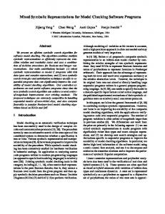
Symbolic

Direct

Naive

I/O cost (sec)

100 10

Experimental Evaluation

For the experimental evaluation we used synthetic datasets generated on the freeway system of Illinois for producing a large number of moving object trajectories (we used the generators provide by [9]). The properties of the datasets appear in Table 1. We evaluate the join queries on two separate sets of the same size. In order to test the efficiency of the proposed technique we vary the workload characteristics. We use 100 queries per run, varying time-interval δt from 50 to 200 time-instants (i.e., from 10% up to 40% of the total dataset lifespan) and

80 60 40 20 0

50

4.

Direct =10

1000

1

distributed in the symbolic space then by choosing the origin appropriately we should be able to decrease the volume of the intersection of each annulus and the data space. Such an origin would guarantee that a small number of false alarms is introduced. This can be accomplished by selecting as the origin an outlier that lies as far away from the data space as possible. Figure 7b shows such an example. It depicts three concentric arcs with center the selected origin O. The locus of points q inside the annuli sections defined by the first and second arcs and the second and third arcs is the set of points for which the origin relative difference of distances from any point p lying on the middle arc is less than the query threshold. It is clear that the curvature of the arcs becomes more flat the further away we move the origin from the center of gravity of the data space. An important observation is that when the origin lies inside the data space, the locus of points defines a complete annulus. On the other hand, when the origin lies far away from the data space the locus of points becomes only a small section of an annulus (and both have the same width). In the first case, the worst case scenario for a circular data space is the largest possible annulus that touches the boundary of the space (Figure 7a). In the second case and a circular data space, for an origin adequately far away from the center of gravity, the worst case scenario is an annulus section that contains the center of gravity and thus has length approximately equal to the data space diameter (Figure 7b). By using this observation as a heuristic we motivate the fact that we chose the string corresponding to the lower left corner of the universe as the origin of the symbolic space. Alternatively, we could compute the center of gravity of the symbolic space on the fly while scanning the index for the symbolic distance computations (here the center of gravity changes according to the t-dimensional points produced, given a query time-interval δt) and choose as the origin the string that lies farthest from that point. Depending on the dimensionality of the symbolic space there might be a large number of candidate boundary strings. For example, for the 2-dimensional space shown in Figure 7 there are four possible boundary strings corresponding to the four corners of the space.

Symbolic 100

10000 I/O cost (sec, log scale)

Table 1: Dataset Characteristics. Total objects 50K Universe size 1000 × 1000 Km Simulation length 500 minutes Initial distribution Uniform Velocity distribution Gaussian

100 150 200 Query time-interval

50

100

150

200

Query time-interval

Figure 8: Symbolic, Direct and Naive for ² = 10.

similarity threshold ² from 10 up to 30 Km (i.e., from 1% up to 3% of the total space). We compare three different techniques, namely the Naive, the Direct, and the Symbolic approaches. For all approaches it is assumed that the actual trajectory data are already stored sequentially on disk in row-major order (i.e., trajectory after trajectory). The naive approach assumes that a total of 1 MB buffer is available and thus it is able to load sequentially from disk a large number of trajectories at a time, instead of assuming that all trajectories are loaded one by one. The Direct approach uses the proposed sliding window algorithm and index structure, but stores the exact trajectory data in the index. Hence, the space requirements of this index is equal to the total size of the actual data (the data needs to be stored twice using two different sequential orderings). This approach is expected to have a smaller verification cost due to a smaller number of false alarms; however, the index cost is expected to be very large. Finally, the Symbolic approach stores only approximations of the trajectories in the index. For the following experiments we use a Symbolic index structure with space requirements one tenth of the space needed for the Direct index. Figure 8(a) measures the total I/O processing cost for all techniques under consideration, for increasing query timeintervals and fixed query threshold ² = 10. To compute the overall times we first computed separately the total number of distinct index I/Os and the total number of verification I/Os. We assume that a random I/O has cost equal to 2 msecs, while a sequential I/O has a cost equivalent to one tenth of a random I/O, i.e., 0.2 msecs. Notice that the time scale for Figure 8(a) is logarithmic. We can see that the proposed index structure helps reduce the total I/O cost by three orders of magnitude. Figure 8(b) shows the results only for the Direct and Symbolic indices. The Symbolic index is about two times faster than the Direct in all cases. Figures 9(a) and 9(b) plot the Symbolic and Direct techniques using query thresholds ² = 20 and ² = 30 respectively. The naive approach is omitted since its behaviour is constant and can be deduced from Figure 8(a). We can observe that the total cost for evaluating the queries increases as expected due to the larger candidate set sizes that result from relaxing the similarity criteria. Also, it is apparent that the cost of the Symbolic approach converges to the cost of the Direct, especially for very large time-interval queries. Nevertheless, the Symbolic approach is still better than the Direct for all cases, even for query time-intervals that span 40% of the total dataset lifespan and 3% of the data space. In the last set of experiments we measure the number of false positives reported by our technique for various values of threshold ². The query time-interval is set to 100 timeinstants or 20% of the lifetime of the trajectories. Figure 10

Symbolic

Direct

Symbolic

Direct

100

100

=30 I/O cost (sec)

I/O cost (sec)

=20 80 60 40 20 0

80 60 40 20 0

50

100 150 Query time-interval

200

50

100 150 Query time-interval

200

Figure 9: Symbolic and Direct ² = 20, 30. Reported pairs

Actual pairs

Answer size (log scale)

100000 10000 1000 100 10 1 5

10

20

30

Figure 10: Reported pairs versus actual pairs. shows the results. The number of reported false positives decreases as ² increases. Furthermore, the number of false positives is in the worst case 200 times the size of the actual result set, which is expected due the approximations introduced and the lower-bounding function used for pruning. In summary, the proposed technique enables efficient evaluation of trajectory join queries for a large number of query predicates. Apart from being better than all other approaches in all cases, it also has minimal storage space requirements, when compared with the Direct approach.

5.

Conclusions

We presented an algorithm and an index structure for efficiently evaluating trajectory join queries. Assuming that a large archive of moving object trajectories has been gathered, we propose a technique that uses symbolic trajectory representations to build a very small index structure that can help evaluate approximate answers to the join queries. Then, by using a post filtering step and loading only a small fraction of the actual trajectory data the correct query results can be produced. Our techniques utilize specialized lower bounding distance functions on the symbolic representations to guarantee no false dismissals. In addition, the index structure enables evaluation of approximate results with sequential disk I/O that improves the overall performance of our algorithm. As future work we plan to extend our techniques for the general trajectory join without temporal constraints.

References [1] L. Arge, O. Procopiuc, S. Ramaswamy, T. Suel, and J. S. Vitter. Scalable sweeping-based spatial join. In Proc. of Very Large Data Bases (VLDB), pages 570– 581, 1998. [2] T. Brinkhoff, H. P. Kriegel, and B. Seeger. Efficient processing of spatial joins using r-trees. In Proc. of ACM Management of Data (SIGMOD), pages 237–246, 1993. [3] V. P. Chakka, A. Everspaugh, and J. M. Patel. Indexing large trajectory data sets with seti. In Proc. of Biennial Conference on Innovative Data Systems Research (CIDR), 2003.

[4] K. Chakrabarti, E. Keogh, S. Mehrotra, and M. Pazzani. Locally adaptive dimensionality reduction for indexing large time series databases. ACM Transactions on Database Systems (TODS), 27(2):188–228, 2002. [5] L. Chen, M. T. zsu, and V. Oria. Symbolic representation and retrieval of moving object trajectories. In Proc. of the ACM SIGMM international workshop on multimedia information retrieval, pages 227–234, 2004. [6] H. D. Chon, D. Agrawal, and A. El Abbadi. Storage and retrieval of moving objects. In Proc. of the International Conference on Mobile Data Management (MDM), pages 173–184, 2001. [7] H. Gunadhi and A. Segev. Query processing algorithms for temporal intersection joins. In Proc. of International Conference on Data Engineering (ICDE), pages 336– 344, 1991. [8] R. H. G¨ uting, M. H. Bhlen, M. Erwig, C. S. Jensen, N. A. Lorentzos, M. Schneider, and M. Vazirgiannis. A foundation for representing and querying moving objects. ACM Transactions on Database Systems (TODS), 25(1):1–42, 2000. [9] M. Hadjieleftheriou. Spatio-temporal generators. http:// www.cs.ucr.edu/ ∼marioh/ generators/ index.html. [10] M. Hadjieleftheriou, G. Kollios, V. J. Tsotras, and D. Gunopulos. Efficient indexing of spatiotemporal objects. In Proc. of Extending Database Technology (EDBT), pages 251–268, 2002. [11] G. R. Hjaltason and H. Samet. Incremental distance join algorithms for spatial databases. In Proc. of ACM Management of Data (SIGMOD), pages 237–248, 1998. [12] E. Keogh, K. Chakrabarti, S. Mehrotra, and M. Pazzani. Locally adaptive dimensionality reduction for indexing large time series databases. In Proc. of ACM Management of Data (SIGMOD), pages 151–162, 2001. [13] E. J. Keogh and M. J. Pazzani. A simple dimensionality reduction technique for fast similarity search in large time series databases. In Proceedings of the Pacific-Asia Conference on Knowledge Discovery and Data Mining, Current Issues and New Applications, pages 122–133, 2000. [14] G. Kollios, V.J. Tsotras, D. Gunopulos, A. Delis, and M. Hadjieleftheriou. Indexing animated objects using spatiotemporal access methods. IEEE Transactions on Knowledge and Data Engineering (TKDE), 13(5):758– 777, 2001. [15] N. Koudas and K. C. Sevcik. Size separation spatial join. In Proc. of ACM Management of Data (SIGMOD), pages 324–335, 1997. [16] J. Lin, E. Keogh, S. Lonardi, and B. Chiu. A symbolic representation of time series, with implications for streaming algorithms. In Proc. of ACM SIGMOD workshop on research issues in data mining and knowledge discovery, pages 2–11, 2003. [17] M.-L. Lo and C. V. Ravishankar. Spatial joins using seeded trees. In Proc. of ACM Management of Data (SIGMOD), pages 209–220, 1994. [18] M.-L. Lo and C. V. Ravishankar. Spatial hash-joins. In Proc. of ACM Management of Data (SIGMOD), pages 247–258, 1996. [19] N. Mamoulis and D. Papadias. Multiway spatial joins. ACM Transactions on Database Systems (TODS),

26(4):424–475, 2001. [20] N. Mamoulis and D. Papadias. Slot index spatial join. IEEE Transactions on Knowledge and Data Engineering (TKDE), 15(1):211–231, 2003. [21] M. Nascimento and J. Silva. Towards historical R-trees. In Proc. of ACM Symposium on Applied Computing (SAC), 1998. [22] D. Papadias, Y. Tao, J. Zhang, N. Mamoulis, Q. Shen, , and J. Sun. Indexing and retrieval of historical aggregate information about moving objects. IEEE Data Engineering Bulletin, 25(2), June 2002. [23] A. Papadopoulos, P. Rigaux, and M. Scholl. A performance evaluation of spatial join processing strategies. In Proc. of Symposium on Advances in Spatial Databases (SSD), pages 286–307, 1999. [24] J. M. Patel and D. J. DeWitt. Partition based spatialmerge join. In Proc. of ACM Management of Data (SIGMOD), pages 259–270, 1996. [25] D. Pfoser, C. S. Jensen, and Y. Theodoridis. Novel approaches in query processing for moving object trajectories. In Proc. of Very Large Data Bases (VLDB), pages 395–406, 2000. [26] J. Shan, D. Zhang, and B. Salzberg. On spatial-range closest-pair query. In Proc. of Symposium on Advances in Spatial and Temporal Databases (SSTD), pages 252– 269, 2003. [27] A. P. Sistla, O. Wolfson, S. Chamberlain, and S. Dao. Modeling and querying moving objects. In Proc. of International Conference on Data Engineering (ICDE), pages 422–432, 1997. [28] Y. Tao and D. Papadias. MV3R-Tree: A spatiotemporal access method for timestamp and interval queries. In Proc. of Very Large Data Bases (VLDB), pages 431–440, 2001. [29] M. Vlachos, M. Hadjieleftheriou, D. Gunopulos, and E. Keogh. Indexing multi-dimensional time-series with support for multiple distance measures. In Proc. of ACM Knowledge Discovery and Data Mining (SIGKDD), pages 216–225, 2003. [30] M. Vlachos, G. Kollios, and D. Gunopulos. Discovering similar multidimensional trajectories. In Proc. of International Conference on Data Engineering (ICDE), pages 673–684, 2002. [31] B.-K. Yi and C. Faloutsos. Fast time sequence indexing for arbitrary lp norms. In Proc. of Very Large Data Bases (VLDB), pages 385–394, 2000. [32] D. Zhang, V. J. Tsotras, and D. Gunopulos. Efficient aggregation over objects with extent. In Proc. of ACM Symposium on Principles of Database Systems (PODS), pages 121–132, 2002. [33] H. Zhu, J. Su, and O. H. Ibarra. Trajectory queries and octagons in moving object databases. In Proc. of Conference on Information and Knowledge Management (CIKM), pages 413–421, 2002.