down depending on the unfailed/failed state of the components. Examples of this conceptual view are provided by the modeling languages described in [l,. 21.
Efficient Transient Simulation of Failure/Repair Markovian Models Juan A . Carrasco Departament d’Enginyeria Electrbnica Universitat Polit6cnica de Catalunya Diagonal 647, plta. 9, 08028 Barcelona, Spain
the size of X grows exponentially with the number of components of the system and both its generation and numerical solution are precluded when the system has more than a few components. Simulation is an approach which by nature is not limited by the size of the model. However, repair rates are typically several orders of magnitude higher than failure rates, which makes the probability of X following a failure transition from any state 2 # U very small. Then, if as it is typical, the system has redundancy to tolerate most single faults, the structure of X is such that only very rarely will X enter D. This makes direct Monte Carlo simulation unfeasible in practice due t o the extremely large number of events which would have to be sampled to get estimates with reasonable confidence intervals. Two types of techniques have been proposed to speed up direct Monte Carlo simulation. Importance sampling techniques exploit heuristic knowledge about the model to modify the sampling distributions so that the rare contributing paths be sampled with significant probabilities. Failure biasing and forced transition are two such techniques which were initially proposed in the context of the nuclear domain [S, 61, and have been recently further developed and applied with success to the simulation of models of fault-tolerant computer systems [7-111. Another importance sampling technique called failure distance biasing which is typically much more efficient than failure biasing has been recently proposed [12]. Estimator decomposition techniques exploit the regenerative behavior of X around U to formulate the metric of interest in terms of lower level metrics which can be estimated more efficiently. Such techniques have been recently used for the estimation of the steady-state availability [8, 101 and the mean time to failure 19, lo]. However, currently proposed methods [5, 101 for transient metrics such as the availability, the expected interval availability and the reliability do not use such techniques and, as it will be discussed, can be highly inefficient. This paper presents new simulation methods for the availability, the expected interval availability, and the reliability combining estimator decomposition techniques with the importance sampling technique described in [12]. The methods are robust and orders of magnitude faster than methods previously proposed
Abstract Simulation methods have recently been developed f o r the solution of the extremely large markovian dependability models which result from complex fault-tolerant computer systems. This paper presents efficient simulation methods for the estimation of transient reliability/availability mefrics f o r repairable fault-tolerant computer systems which combine estimator decomposition techniques with an efficient importance sampling technique recently developed. Comparison with simulation methods previously proposed for the same type of metrics and models shows that the methods proposed here are orders of magnitude faster.
1 Introduction This paper considers the evaluation of repairable fault-tolerant computer systems which from the user’s point of view can be seen as either up or down. Several dependability metrics such as the steady-state availability, the availability, the expected interval availability, the mean time to failure and the reliability can be appropriate to evaluate the up/down behavior of these systems. For the computation of these metrics, the system can be conceptualized as made up of components which change their state as a result of failure and repair processes. These processes may involve in general several components and the system is up or down depending on the unfailed/failed state of the components. Examples of this conceptual view are provided by the modeling languages described in [l, 21. Under the assumption of exponential failure and repair time distributions, the behavior of the system can be described by a continuous-time Markov chain (CTMC) X I whose transitions represent either failures or repairs of components. The state space of X can be partitioned into the set of up states U and the set of down states D . Let U E U be the state in which all components are unfailed. We assume that all components are repairable and that at least one failed component is under repair in any state 2 # U . Failure propagation, the impact of the operational configuration of the system into failure and repair processes, and limited repairmen introduce dependencies in the model such that, in general, X has to be solved using general-purpose, state-level methods. Current stateof-the-art numerical methods [3,4] can solve CTMC’s with tens of thousands of states. However, in general,
I52
CH3021-3/91/000010152/$01.00 0 1991 IEEE
for the same metrics. The rest of the paper is organized as follows. Section 2 reviews importance sampling theory and previous simulation methods. Section 3 argues qualitatively the inefficiency of previous methods and presents the estimator decomposition techniques on which the new simulation methods are based. Section 4 examines the problem of deriving confidence intervals for the estimates. Section 5 presents experimental results illustrating the robustness and efficiency of the proposed methods. Section 6 concludes the paper. The formulations on which the estimator decomposition techniques are based are derived in the Appendix.
2
Background
Since all metrics considered in this paper have usually values very close to 1, we use the complementary metrics (unavailability, expected interval unavailability, and unreliability) in our presentation. For all metrics we assume that X is initially in the state U . The unavailability a t time t , u a ( t ) is the probability that X is in D at time t . The expected interval unavailability a t time 1, i t i a ( t ) is defined as m d i ( t ) / t , where m d t ( t ) is the mean down time by time t , i.e., the expected value of the time spent by X in D during the interval [ O , t ] . I t can be easily shown that:
mdt(t) =
I’
ua(r)dr .
(1)
Finally, the unreliability at time t , u r ( t ) , can be defined as the probability that X has hit D during the interval [0, t ] . All the metrics previously defined can be expressed as the expected value of a function defined over the set of paths of X and, therefore, can be estimated by simulating X and taking the sample mean of the corresponding path function. However, only paths which hit D have non-null contributions and, given the structure of X , an extremely large number of events (transitions) would have to be sampled to generate the number of contributing paths required to achieve reasonable confidence intervals. The simulation can be speeded up by using importance sampling techniques. The principles behind importance sampling [13] can be illustrated using a simple example. Assume we want to estimate the expected value of Z ( 0 ) , where 0 is a random variable with density f(8). Let f * ( O ) be a different density function such that f*(O) # 0 whenever Z ( O ) f ( O ) # 0 and, for the values 8 satisfying the latter condition, let A*(O) = f(O)/f*(O) be the likelihood ratio. We have:
which tell us that un unbiased estimator of E [ Z ( O ) ] can be obtained by sampling 0 using T(O)and taking the sample mean of the function Z*(O) = Z(O)A*(O). The variance after n samples is:
which is null when f*(O) = f ( O ) Z ( O ) / E [ Z ( @ ) ]i.e., , when the values of 0 are sampled with likelihoods equal to their relative infinitesimal contributions to E Z 0 . This is impossible in practice because E [ Z ( S ] ]is unkown, but when choosing a practical f.10) we should try t o match as closely as possible f( )Z(O)/E[Z(@)]. In the context of this paper, this means that we should drive the simulation effort to the contributing paths (those hitting 0 )and, furthermore, assign higher likelihoods to the paths with higher contributions to the metric under estimation. We next review briefly the simulation methods proposed in [5, 101 for u r ( t ) and iua(t). The method proposed in 51 for the simulation of ur(t samples paths of X til either the path hits D or t e sum of all sampled holding times exceeds t . Let A, denote the output rate from the state E and t , the sum of the previously sampled holding times. The holding times in states 2 # U are sampled from their exponential distribution f(y) = Aze-’=Y, but the holding times in U are sampled using the conditional 1 - e - ’ ~ ( ~ - ~ c which )), distribution f*(y) = X,,e-’-Y/( results when the holding time in U is restricted to be < t-t,. This importance sampling technique is called transition forcing and is used to avoid sampling paths which will not hit D by time t and thus will have null contributions to u r ( t ) . Transitions are sampled using another importance sampling technique called failtire biasing. Failure biasing is applied when the current state has both outgoing failure and repair transitions and consists in biasing the transition probabilities so that the probability of following a failure transition be FBIAS and that of following a repair transition be 1 - F B I A S , with the biasing probabilities within each class distributed proportionally to the unbiased probabilities. The biasing scheme is turned off as soon as a down state is hit. The heuristic behind failure biasing is to increase the sampling probabilities of the paths which enter D. A value F B I A S = 0.5 typically minimizes the required simulation effort. The simulation method for u r ( t ) proposed in [lo] is sligthly different. The method simulates X till entry in D and does not sample the holding times in U . The number of visits IC to U during a path is recorded and the contribution of the path to u r ( t ) is computed by conditioning out the distribution of the total time spent in U , which follows a k-stage Erlang distribution with parameter A,,. The method for iua(t) proposed in [lo] conditions out a predefined value L of holding times in U and samples successive holdin times in U till the sum of all sampled holding times fincluding those in states t # U exceeds t . Two importance sampling techniques in a dition to failure biasing have been experimented in [lo]. The first one is identical to failure biasing except that F B I A S is distributed uniformly among the failure transitions. The second is an ellaboration of failure biasing in which a given probability is allocated t o the transitions corresponding to failures of component types with already some component failed. The latter is only meaningful when redundancy is only provided between components of the same type (i.e., undistinguishable), quite a restrictive assumption which is not fullfilled, for instance, by
h
1
the large example presented in Section 5. Failure distance biasing is a more ellaborated biasing scheme which exploits the concept of failure distance. See [12] for a more detailed description of the scheme, including implementation and optimization issues. In failure distance biasing components are classified into failing and non-failing, depending on whether they fail on their own or can only be failed by propagation of failures of other components. The failure distance from an operational state x is defined as the minimum number of failing components whose failure in x would take the system down. A failure transition is said dominant if it reduces the failure distance and critical if it reduces the failure distance by more than one. The criticality of a failure transition is defined as the amount by which it reduces the failure distance. Failure distance biasing is done in steps. At each step a subset of transitions is split into two subsets, which are biased in relation to one another (keeping as in failure biasing the relative values of the transition probabilities within each subset), and one of the subsets is passed to the next step. If one of the subsets is empty, the step is skipped. The first step is failure biasing. In the next step, the subset of dominant failure transitions is assigned a probability DBIAS in relation t o the current set (failure transitions) and passed to the next step, and the subset of non-dominant transitions is assigned a relative probability 1 - D B I A S . The third step is repeated while the transitions in the current set have different criticalities and assigns the relative probability 1 - CBIAS to the subset of failure transitions with smallest criticality and CBIAS to the complementary subset, which is passed for the next application of the biasing step. Assume, for instance, that a state has outgoing repair transitions, non-critical dominant transitions, and critical failure transitions of criticalitites 2 and 3. These subsets of transitions would be sampled with probabilities 1- F B I A S , FBIAS( 1 - C B I A S ) , F B I A S C B I A S ( 1 - C B I A S ) , and FBIAS C B I A S 2 , respectively. The heuristic behind failure distance biasing is t o sample more often the shortest paths entering D.By taking values of DBIAS and CBIAS more or less close to 1, the biasing scheme can focus more or less the simulation effort to these paths. Using an independent biasing parameter to deal with critical transitions is convenient since the actual importance of these transitions depends on the values of the “coverage” parameters of the model. The scheme has been compared in [12]with failure biasing for the simulation of the steady-state unavailability and has been shown to be typically much more efficient.
3
next an approximate analysis for u r ( t ) which clarifies this point and provides further insight. Let v,” be the number of sojourns in U before X hits D and T,D the time a t which X hits D. We can formulate u r ( t ) as:
k=l
where
Q k ( t ) = P[T,D _< t 1 v,” = k]P[v,” = k ] .
6
Q k 2) can be interpreted as the contribution to u r ( t ) o f t e set of paths hitting D after k sojourns in U . Let 7 be the probability that a path starting in U hits D before U. From the memoryless property of CTMC’s, it follows that v,” has a geometric distribution with parameter y. Since repair rates are typically several orders of magnitude higher than failure rates and all states x # U have a t least one outgoing repair transition, the mean holding times in the states x # U are usually much smaller than the mean holding time in U , h,. In addition, given the structure of X , paths which visit many states 2 # U before hitting D after a given number k of sojourns in U have much smaller probabilities than paths of the same type visiting few states x # U . This allows to neglect the holding times in the states x # U and approximate T,D conditioned t o v,” = IC by the sum of k holding times in U . It follows that TuD conditioned to :v = k has approximately a k-stage Erlang distribution with parameter A,, = h;’, and:
The expected value of v,” when the paths are sampled with probabilities proportional to their relative contributions (optimal distribution to which an efficient importance sampling scheme would tend to adjust) is -
v,” = k Q k ( t ) / C F = l & k ( t ) . Figure 1 plots .,” as a function of y and t/h,, using the approximation developped for Q k ( t ) . It is clear that when t is smaller or of the order of magnitude of h, only paths with few regenerative cycles around U have important contributions to u r ( t ) . However for small values of y (which are typical in the models considered here), longer and longer paths have important contributions to u r ( t ) as t / h , becomes >> 1. The same can be argued to happen when simulating u a ( t ) and i u a ( t ) . The conclusion is that simulation methods for transient metrics using biasing schemes which tend to focuss the simulation effort towards short paths entering D can be expected to degradate when t >> h, due to: a) an increase in the simulation effort per path, b) a decrease in the efficiency of the biasing scheme. We present next formulations for u a ( t ) , i a a ( t ) , and ar(t) in terms of lower-level metrics which follow a
Estimator Decomposition
Failure distance biasing and, t o a lesser extent, failure biasing and the related biasing schemes described in [lo] tend to concentrate the simulation effort towards the shortest paths entering D. These paths have the more important contributions to u a ( t ) , iua(t) and u r ( t ) only when t is smaller or of the order of magnitude of the mean holding time in U , h,. We present
IS4
]
-
Each low-level metric transform M ( s ) can be formulated as the expected value of a function Z ( fined over the set of paths t o absorption of one o two detransient discrete-time Markov chains (DTMC's), i.e., we can write:
n
p0.l
FER
0.01
0.1
1
10
Jhu Figure 1: Approximate average number of sojourns in U per path during the simulation of ~ ( twhen ) paths are sampled according to their contributions.
neat heuristic and can be simulated more efficiently. Let
gl(t) the probability that given X ( 0 ) = U , X ( t ) E D and X has not hit U by time t , g2(t) the probability density function of the duration of a regenerative cycle around U , h l ( t ) the probability that given X ( 0 ) = U , X has hit D by time t without hitting U before, h2(t) the probability that given X ( 0 ) = U , X has hit either D or U by time t .
where R is the set of paths to absorption of the corresponding transient DTMC and P ( r ) is the probability of the path r . Two transient DTMC's with initial state U are used. The first one, X ' , describes (ignoring holding times) the behavior of X till its first hit in U. The second one, X", describes the behavior of X till its first hit in either U or D and has two absorbing states: Q , representing hit in U , and d, representing hit in D . Let L r ) denote the length of path r (number of transition&, z , ( r ) the state visited in path r after the ith transition (zo(r) = U ) , X i j the transition rate from i to j , and q i j . = X i j / X i the conditional transition probability from z to j. We have P ( r ) = I l o < i < L ( r ) qz,(r),z,+a(r). The path fun'tion required for each low level metric can be derived by considering that the holding times in the states z , ( r ) ,i = 0,. . . , L ( r ) - 1 conditioned to the execution of r are independent exponential random variables with parameters AZ,(,.). Table 1 gives the transient DTMC and the path function required for each denotes the low-level metric. In the table, Pz.,(r)/r(s) Laplace transform of the probability that the associated transient CTMC is in q ( r ) at time t , conditioned to the execution of r by the embedded DTMC. These Laplace transforms can be computed using:
In the Appendix we formulate the Laplace transforms of u a ( t ) and u r ( t ) in terms of the Laplace transforms of the above low-level metrics. Denoting by F ( s ) the Laplace tranform of f ( t ) , we obtain:
i = 1, . . . , L ( r ) - 1 , (3) Remembering that iua(t) = m d t ( t ) / t ,it becomes clear that the simulation of i u a ( t ) is virtually equivalent to the simulation of m d i ( t ) . Let II(s) = Gl(s)/s, using (1, 2), we have:
Efficient numerical algorithms for numerical Laplace transform inversion exist (see, for instance, [14] which allow to compute the value of a function f(t] a t a given abscissa t from a few values of its Laplace transform F ( s ) . Then, estimates for u a ( i ) , u r ( t ) , and be obtained from estimates for the Laplace in the right-hand sides of ( 2 , 3, 4) at the abscissae required by the inversion algorithm.
so that the computation of any path function of Table l has linear cost on the path length. In the methods proposed here, an independent simulation stream is used to estimate the Laplace tranforms of each low-level metric. Given the structure of X , only the regenerative cycles around U with few transitions have significant probabilities and the duration of these cycles follows very closely an exponential distribution with mean h,. Thus, all paths r of X ' with significant contributions to G ~ ( shave ) a similar functional value Zr(s) and, according to importance sampling theory, direct Monte Carlo simulation can be expected to be very efficient. A similar reasoning based on the typical behavior of X supports the efficiency of direct Monte Carlo simulation of H z ( s ) . Importance sampling techniques are however required for the efficient estimation of, G l ( s ) ,H l ( s ) , and I l ( s ) , since only the paths of X' and X " hitting D have nonnull contributions to these metrics. In addition, the
antitransforms we obtain for = ( t ) an expression of the form: h ( t ) f?(t) &t> (5)
probabilities of these paths (and their relative contributions) are typically strongly ranked according to the number of failure transitions they contain. This is in accordance with the heuristic behind failure distance biasing and we can expect the simulation of Gl(s), H l ( s ) , and I l ( s ) under that biasing scheme to be particularly efficient.
4
+
+
1
A
h
where h ( t ) is non-random and f i ( l ) , f 2 ( t ) are random variables, which, denoting by (.ZM)~(S) the path function associated to the metric M ( s ) as given in Table 1 and by ( Z & ) r ( ~ )the function affected by the likelihood ratio, can be interpreted as the sample mean estimates of, respectively, the path functions:
Derivation of Confidence Intervals
This section discusses the derivation of confidence intervals for the estimates of the metrics. Consider, for instance, t& derivation of confidence intervals for U Q ( ~ ) . Let GI s) and sample mean esdefine AG,(s) = timates of Gl(s\ and g ( s ) - Gl(s), AG,(s) = - G ~ ( s ) . We have h
G(s)
(2):
A similar development holds for the other metrics, where the random terms in (5) can be interpreted as the sample mean estimates of the path functions:
AGl(s) and AGz(s) have null expected values and the same standard deviations as, respectively, G l ( s ) and G(s). For any estimate of E ( s ) of reasonable quality, the relative standard deviations of c ( s ) and Gz(s) will be small so that we can approximate by its first-order Taylor expansion on AGl(s) h
-
for s(t) and:
Replacing AGl(s) and AGz(s) by, respectively, - G l ( s ) and - Gz(s) and taking Laplace
G^;(s)
G(s)
1.56
for Z t ( t ) .
ith substream, s2 is the sample variance of (W1)r(t) obtained in the Xth substream, and f i is the value given by a symbolic estimator (which takes into account all the samples) of E[((Wl),(t)2 for the values of the biasing parameters used in t e ith substream. See [12] for details. Using :s R, - Rk is more robust than using sz, which can be dangerous when the model is badly-behaved and the variance is only well estimated after a large number of sampled paths.
Then, A ( t ) and A(t) have asymptotically a normal distribution and approximate confidence intervals for the metrics can be derived by using the normal distribution with variance: $2
= $;
+
+ $;
where $; and $22 are estimates for the variances of, respectively, f?(t) and These estimates can be obtained by sampling the path functions (6-ll), The computation of these path functions requires the knowledge of Gl(s) and.Gz(s), H l ( s ) and HZ s), or I l ( s ) and G ~ ( srespectively, ), which are precise(yl the quantities under estimation. This problem is solved as follows. We organize each simulation stream in substreams, each having a length which approximately doubles the length of the previous substream for the same low-level metric. The streams for the two low-level metrics run in parallel with optimal allocation of events according to their contributions to the variance of the metric estimate. The first substreams use initial rough estimates for the Laplace transforms of the low-level metrics obtained running short presimulation substreams. The following substreams use the estimates for the Laplace transforms available at the end of the previous substreams. The Laplace transforms Gz(s),H z ( s are estimated by the sample means of the correspon ing path function and, at the end of the kth substream, 3; is computed by:
h(t).
5
h1
Experimental Analysis
In our implementation of the simulation methods we compute Laplace antitransforms using the inversion formula [14]: CO
where a is a parameter which is chosen large enough to make the relative discretization error smaller than DERROR = The convergence of the series is accelerated by the epsilon algorithm, and the accelerated series is truncated when the relative difference between the two last truncated values is smaller than TERROR = The value for a and the number of abscissae at which the Laplace transforms are bookkept are chosen after running the presimulation substreams and rough estimates for the Laplace transforms are available. For the presimulation we use oversized values for these parameters. Recovery procedures are implemented in case the values chosen after the presimulation turn out to be insufficient to achieve the specified accuracy. In all cases we have tested, between 20 and 30 terms have been enough to achieve convergence. More sophisticated inversion formulae [15] could be used to get estimates of the metrics at several values o f t using slightly more Laplace transforms. A number of experiments have been carried out using models of small size and comparing the results obtained by the simulation methods presented here with those obtained numerically by METFAC [16] and we have found that the methods are robust. This will be illustrated using the fault-tolerant database example described in [7]. The system is made up of two frontends, two databases and two processing subsytems and each processing subsystem includes one switch, one memory and two processors. The system is up if at least one front-end, one database, and one processing subsystem are operational, and a processing subsystem is operational if the switch, the memory, and at least one of the processors are operational. All components fail with rates 1/2400 hrs-l, except the processors which fail with rate 1/120 hrs-’. A processor failure is propagated to one database with probability 0.01. There is a single repairman which uses a preemptive discipline with priority given first to databases and front-ends, next to memories and switches, and last to processors. Components of the same priority are chosen at random and all components have a meail repair time of 1 hour.
d
where M is the total number of sampled paths and s i is the sample variance of ( W Z ) ~computed (~) in the kth substream. Computing a sample variance using all sampled paths is not possible because, being different the estimates for the Laplace transforms of the lowlevel metrics used in each substream for the computation of (W2 ( t ) , we are in fact sampling a different random varia le (W2),.(t)at each substream. Simulation of Gl(s), H l ( s ) , H l ( s ) is optimized using an adaptive scheme in which the values of the biasing parameters are updated at the end of each substream to minimize the variance of the sampled path function. The estimates for these Laplace transforms are computed by weighting optimally the sample means obtained for the different substreams so as to minimize $;f. This is done t o take into account the decrease in variance of the sampled path function resulting from the progressive optimization of the biasing parameters. The estimate for the variance 5: at the end of the kth substream is computed by:
b.
where a; is the weight associated to the sample mean of the ith substream, Mi is the number of paths of the
157
The proposed simulation methods were run for a wide range of values of t with a goal of a 99% confidence interval of f2% and a limit of 500,000 events. Tables 2, 3, and 4 give the exact values computed by numerical methods, the estimates obtained by simulation, and the number of simulated events required to achieve the specified tolerance (including the events sampled in the presimulation substreams). In all cases, the exact value is within the predicted interval confidence and a small number of events is enough to achieve the specified tolerance. Our methods differ from those previously proposed [5, 101 in the use of estimator decomposition techniques and the use of the failure distance biasing scheme. A comparison isolating the impact of each improvement will be presented using a large reallistic example. The example is the fault-tolerant data processing system whose architecture is shown in Figure 2. A dual configuration of data processing units (DPU’s) command control subsystems located at remote sites. Each control subsystem comprises two redundant control units (CU’s) working in hot-standby redundancy. The system can be accessed through two redundant front-ends connected to the DPU’s. The DPU’s and CU’s communicate using a redundant local area network (LAN) to which each DPU and each CU has access through dedicated communication processors (CP’s). Components fail with constant rates xFE = 2 x 10⁻⁴, ~ D p u= 10-3, xCU = 2 x 10⁻⁴, Xcp = 5 x and XL = respectively. Two failed modes are considered for the DPU’s: “soft” and “hard”. The first mode occurs with probability 0.9 and can be recovered by an operator restart; the second mode occurs with probability 0.1 and requires hardware repair. Coverage is assumed perfect for all faults except those of the DPU’s, which take the system down with a probability of 0.01. Lack of coverage is modelled by propagating the failure of one DPU to the other DPU. There are three repair teams. The first repairs LAN’s and CP’s, with preemptive priority given t o LAN’s. The second repairs FE’s, DPU’s and CU’s in “hard” failed mode, with preemptive priority given first to DPU’s, next t o FE’s, and last to CU’s. The third makes DPU restarts. Each team includes only one repairman. Failed components with the same repair priority are taken at random for repair. Components are repaired with rates FE = 0.5, P D P U h = 0.5, P D P U S = 4, PCU = 0.5, P c p = 0.5, and P L = 0.2, respectively. The system is considered up if one unfailed DPU can communicate with a t least one unfailed CU of each control subsystem. Different LAN’s can be used for communication between the active DPU and the active CU of each control subsystem, but the communication has to be direct, i.e., involving only one C P of each unit and one LAN. The resulting CTMC has about 4.6 x 10” states, which clearly precludes both its generation and numerical solution. Due to space limitations we will only present experimental results for u r ( t ) . Comparison of our methods for i u a ( t ) with that proposed in [lo] gives qualitatively
identical results. The method proposed in [5] for u r ( t ) (making abstraction of the biasing scheme used to sample transitions) will be denoted by F (forcing). The method proposed in [lo] for ur(t (also making abstraction of the biasing scheme use to sample transitions) will be called P C (partial conditioning). The latter allows the computation of estimates at several t , but in our experiments we only computed the metric at a given value t and the simulation of the path under PC was aborted when the sum of the sampled holding times exceeded t , since in this case the path currently sampled has a null contribution. We run F and P C with failure biasing (FB , the same methods with failure distance biasing ( DB), and the proposed method based on (3) and using failure distance biasing for several values o f t with a goal of a 99% confidence interval of &2% and a limit of 500,000 events. Our implementation of F and P C under both FB and FDB includes an adaptive optimization scheme for the biasing parameters. We turned biasing off in our method when MAXREP = 2 repair transitions are sampled in the same path. This improves the robustness of the biasing scheme without affecting its efficiency significantly. This was however not done under F and P C since it would turned the biasing scheme off prematurely when t >> U and long paths have to be sampled. The CPU time per simulated event in our method is about 50% higher than in F and P C due to the computation of the Laplace transforms and the invocations of the Laplace transform inversion algorithm, and we present CPU times instead of sampled events for comparison purposes. These times were measured on a SUN 3/260. Figure 3 shows the results, using estimates for the required CPU times when the goal confidence interval was not achieved after 500,000 events. The speedup of the proposed method over previous ones ( F and P C with failure biasing) is between 3 and 4 orders of magnitude. In fact none of the previous methods can achieve the goal confidence interval in a practical amount of time whereas our method achieves it in about 2 minutes in all cases. F and P C with failure distance biasing are slightly better than the proposed method when t is smaller or of the order of magnitude of h, (172 hours). As 1 increases, the performance of F and P C with failure distance biasing rapidely deteriorates for the reasons explained in Section 3. Figure 4 gives the average path lengths, clearly confirming the arguments given there.
d
Ez
6
Conclusions
We have proposed new methods for the transient simulation of repairable fault-tolerant systems which are robust and efficient for any value o f t . For a typical large example speedups of 3 to 4 orders of magnitude over previously proposed methods have been reported. These speedups are the result of using estimator decomposition techniques and the more efficient failure distance biasing scheme. Previously proposed methods under failure distance biasing tend to be slightly more efficient than the method proposed here only
I58
Table 2: u a ( 2 ) simulation results for the fault-tolerant database system.
t 0.01 0.1 1 10 100 103 104 105
exact 1.284 x lo-'' 1.219 x lo-" 7.399 x 10⁻⁷ 3.425 x 3.431 x 3.431 x 3.431 x 3.431 x
estimate 1.304 x lo-'' f 2.6 x 1.235 x f 2.4 x 7.389 x f 1.5 x 3.365 x f 6.7 x 3.373 x f 6.7 x 3.373 x l o b 6 f 6.7 x 3.373 x f 6.7 x 3.373 x f 6.7 x
events lo-'' lo-"
lo-' lo-" lo-" lo-" lo-"
18,643 18,208 21,530 61,476 62,611 62,611 62,611 62,611
Table 3: u r ( t ) simulation results for the fault-tolerant database system.
t
exact
0.01 0.1 1 10 100 103 104 105
1.289 x lo-'' 1.261 x lo-" 1.023 x 2.960 x 3.353 x 3.387 x 3.340 x 0.2881
estimate 1.294 x lo-'' f 2.6 x 1.266 x lo-" f 2.5 x lo-'' 1.022 x f 1.9 x lo-" 2.976 x f 5.9 x 3.351 x f 6.7 x 3.388 x f 6.7 x 3.336 x f 6.6 x 0.2862 f 5.6 x
events 10,094 9,813 15,963 36,559 39,051 38,706 37,811 26,061
Table 4: i u a ( t ) simulation results for the fault-tolerant database system.
t 0.01 0.1 1 10 100 lo3 lo4 lo5
exact 4.287 x lo-'' 4.124 x lo-' 2.842 x 2.639 x 3.351 x 3.423 x 3.430 x 3.431 x
estimate 4.354 x lo-'' 4.182 x lo-' 2.859 x 2.608 x 3.307 x 3.372 x 3.386 x 3.373 x
I so
f 8.6 x f 8.1 x f 5.3 x f 5.2 x f 6.6 x f 6.7 x It 6.6 x
lo-" lo-' lo-" lo-" lo-" lo-" f 6.7 x lo-"
events 18,643 18,572 18,622 54,592 61,866 62,645 66,517 62,606
811a
CP12a
851r
BS2a
CUI1
cul2 * * * CUSl
CU52
CPllb
CP12b
851b
CP52b
”o l
-t-
proPo=d PCwithFDB PCwithFB
4
4 t (h)
Figure 3: CPU times required to achieve a 99% f2% confidence interval in the simulation of u r ( t ) for the fault-tolerant data processing system.
t
ours.)
Figure 4: Average path lengths in the simulation of u r ( t ) for the fault-tolerant data processing system. convolution operator, we can write:
when t is small or of the order of magnitude of the mean holding time in the state with all components unfailed h, , but their performance rapidly deteriorates as t increases. This behavior is specially problematic for the reliability, since this metric is often used to characterize the long-term dependability behavior of the system and values of 1 several orders of magnitude higher than h, will be typically of interest, particularly for large systems, where A, can be large.
00
pi(t)
=
P [ X ( t )= i A X has hit
U
k=O
6 times in [O,t]I X ( 0 ) = U] = 00
= Cg?’(t)
* 4:i(t).
k=O
The point unavailability u a ( t ) can be computed as
C i E D p , (and, t ) according to its definition, g l ( t ) =
APPENDIX In this appendix we obtain the formulations 2), (3) for the Laplace transforms of, respectively, u a [ t ) and ur(t). Let p ; ( t ) = P [ X ( t )= i I X ( 0 ) = U ] and q5:i(t) the probability that, given X ( 0 ) = U , X ( t ) = i and X has not hit U in [ O , t ] . Remembering the definition of g 2 ( t ) given in Section 3 and denoting by g?’(t) the n-fold convolution of g 2 ( t ) with itself and by * the
CiED q5:i(t). Then, using
(12):
The formulation for the Laplace tranform of zlr(l) can be obtained by resorting to semi-Markov process
[5] E.E. Lewis and F. Bohm, “Monte Carlo Simulation of Markov Unreliability Models,” Nuclear Engineering and Design, vol. 77, 1984, pp. 4962. [6] T . Zhuguo and E.E. Lewis, “Component Dependency Models in Markov Monte Carlo simulation,” Reliability Engineering, vol. 13, 1985, pp. 45-62.
Figure 5: Transition graph of the semi-Markov process Y’. theory [17]. Let Y be the transient CTMC with state space U U { d which is obtained from X by collapsing D into an a sorbing state d and consider the semiMarkov process Y’ whose transition graph is given in Figure 4 and is defined so that, provided Y ( 0 ) = U : a) Y ’ ( t ) = U’ if Y ( t ) E U , b) Y ’ ( t ) = d if Y ( t ) = d , and c) Y’ makes a transition into U‘ whenever Y enters U . The functions h l ( t ) and h2(t) defined in Section 3 can be expressed in terms of the kernel functions of Y’ as: h l ( t ) = qu’d(t) (13) h 2 ( t ) = qu#u,(t) -k qurd(t). (14) By construction, u r ( t ) is the transition probability p u f d ( t ) . Then, using semi-Markov process theory we can write:
[7] A.E. Conway and A. Goyal, “Monte Carlo Simulation of Computer System Availability/Reliability Models,” Proc. 17th Int. Symp on Fault-Tolerant Computing F T C S - 1 7 , 1987, pp. 230-235.
b
u r ( t ) = pu’d(t) = qu’d(t)
+
[8] A. Goyal, P. Heidelberg, and P. Shahabuddin, “Measure Specific Dynamic Importance Sampling for Availability Simulations,” Proc. 1987 W i n t e r Simulation Conference, A. Thesen, H. Grant and W. D. Kelton (eds.), pp. 351-357. [9] P. Shahabuddin, V.F. Nicola, P. Heidelberger, A . Goyal, and P.W. Glynn, “Variance Reduction in Mean Time to Failure Simulations,” Proc. 1988 W i n t e r Simulation Conference, M. Abrams, P. Haigh, and J . Comfort (eds.), pp. 491-499.
lt
[lo] A. Goyal, P. Shahabuddin, P. Heidelberger, V.F. Nicola, and P.W. Glynn, “A Unified Framework
pu’d(t - 7)dqulul(T) .
for Simulating Markovian Models of Highly Dependable Systems,” IBM Research Report RC 14772, Yorktown Heights, Nov. 1989.
Considering that qutuj(0) = 0 and taking Laplace transforms we obtain:
uR(s) = =
Quid(S) Qutd(S)
[ll] R. M. Geist and M. K. Smotherman, “Ultrahigh Reliability Estimates Through Simulation,” Proc. A n n . Reliability and Maintainability S y m p . , January 1990, pp. 1-6.
4-s p ” ~ d ( s ) Q u ~ u ~=( s ) 4-sUR(s)Qujut(s) .
Finally, solving in UR(s) and using (13, 14):
UR(s ) =
[12] J . A . Carrasco, “Failure distance-based Simulation of Repairable Fault-Tolerant Systems,” Proc. 5th Int. Conf. on Modelling Techniques and Tools for Computer Performance Evaluation, 1991, pp. 337-351.
Qu’d(s) = H1 1 - s Q ~ ~ ~ ~1 ( ss ( )H ~ ( s ) H ~ ( s ) ’)
[13] J.M. Hammersley and D.C. Handscomb, Monte Carlo Methods, Metheun, London, 1975.
References
[14] K.S. Crump, “Numerical Inversion of Laplace Transforms Using a Fourier Series Approximation,” J . of the A G M , vol. 23, no 1, January 1976, pp. 89-96.
[l] A. Goyal, W.C. Carter, E. de Souza e Silva, S.S. Lavenberg, and K.S. Trivedi, “The System Availability Estimator,” Proc. 16th Int. S y m p on Fault-Tolerant Computing F T C S - 1 6 , 1986, pp. 84-89.
[15] F. DeHoog, J . Knight, and A.N. Stokes, “An inproved method for numerical inversion of Laplace transforms,” S I A M J. Sci. Stat. Comput., vol. 3, no. 3, pp. 357-366, 1982.
[2] J.A. Carrasco, “Hierarchical, Object-oriented Modeling of Fault-Tolerant Computer Systems,” Proc. CompEuro 91 Conference, 1991, pp. 452456.
[16] J.A. Carrasco and J . Figueras, “METFAC: Design and Implementation of a Software Tool for Modeling and Evaluation of Complex FaultTolerant Computing Systems,” Proc. 16th I d . Symp. on Fault-Tolemd Computing F T C S - 1 6 , 1986, pp. 424-429.
[3] W.J. Stewart and A. Goyal, “Matrix Methods in Large Dependability Models,” IBM Research Report RC 11485, Yorktown Heights, Nov. 1985. [4] A. Reibman and K. Trivedi, “Numerical Transient Analysis of Markov Models,” Computer Opemtions Research, vol. 25, no. 1, pp. 19-36, 1988.
[17] E. Cinlar, Introduction t o Stochastic Processes, Prentice-Hall, Englewood Cliffs, 1975.
161