... of Electrical Engineering. University of Notre Dame. Aug 13, 2009. Sunil Srinivasa and Martin Haenggi. (). University of Notre Dame. IT School 2009. 1 / 22 ...
Path Loss Exponent Estimation in Large Wireless Networks Sunil Srinivasa and Martin Haenggi Network Communications and Information Processing (NCIP) Lab Department of Electrical Engineering University of Notre Dame
Aug 13, 2009
Sunil Srinivasa and Martin Haenggi
()
University of Notre Dame
IT School 2009
1 / 22
Motivation Large-scale path loss law: signal strength attenuates with distance d as dγ � �−γ d . S∝ d0 Though it is typically assumed in analysis and design problems that the path loss exponent (PLE) is known a priori, it is often not the case. The PLE has a strong impact on the quality of links, and therefore needs to be accurately estimated for the efficient design and operation of systems.
Sunil Srinivasa and Martin Haenggi
()
University of Notre Dame
IT School 2009
2 / 22
Motivation (contd.)
Example 1: The information-theoretic capacity of large random ad hoc networks scales as ∗ n2−γ/2 √ n
for for
26γ 3.
Depending on the value of γ, different routing strategies are required to be implemented.
¨ ur, O. L´evˆeque and D. Tse, “Hierarchical Cooperation Achieves A. Ozg¨ Optimal Capacity Scaling in Ad Hoc Networks,” IEEE Trans. Info. Th., 2007. ∗
Sunil Srinivasa and Martin Haenggi
()
University of Notre Dame
IT School 2009
3 / 22
Motivation (contd.) Example 2: Outage probability in a planar Poisson point process with Rayleigh fading. λ = 1, p = 0.05, m = 1, N0 = −25 dBm 1
Θ = 20 dB Θ = 10 dB Θ = 5 dB Θ = 0 dB Θ = −5 dB
0.9
Outage probability
0.8 0.7 0.6 0.5 0.4 0.3 0.2 0.1 2
2.5
3
3.5
γ
4
4.5
5
The system performance critically depends on γ. Sunil Srinivasa and Martin Haenggi
()
University of Notre Dame
IT School 2009
4 / 22
System Model
Receiver
Transmitter
Filled circles: transmitters. Empty circles: receivers. Sunil Srinivasa and Martin Haenggi
()
An infinite Poisson point process (PPP) on R2 with density λ. Channel access scheme is ALOHA. p is the ALOHA contention parameter. Therefore, the set of transmitters forms a PPP with density λp. No synchronization.
University of Notre Dame
IT School 2009
5 / 22
System Model (contd.)
Attenuation in the channel: product of large-scale path loss, with PLE γ. small-scale fading (m-Nakagami). m = 1: Rayleigh fading ; m → ∞: no fading.
Noise is AWGN with variance N0 . All the transmit powers are equal to unity (no power control). Problem: How do you accurately estimate the PLE at each node in the network in a completely distributed manner?
Sunil Srinivasa and Martin Haenggi
()
University of Notre Dame
IT School 2009
6 / 22
What Makes Estimating the PLE Complicated? The large-scale path loss is commonly taken to be deterministic while the small-scale fading is modeled as a stochastic process. This distinction, however, does not hold when the nodes themselves are randomly arranged. So, we need to consider the distance and fading ambiguities jointly. Moreover, PLE estimation needs to be performed during the initialization of the network. During this phase, the system is typically interference-limited due to the presence of uncoordinated transmissions. Purely RSS-based estimators cannot be used in these situations.
Sunil Srinivasa and Martin Haenggi
()
University of Notre Dame
IT School 2009
7 / 22
Overview
Propose three distributed algorithms for estimating the PLE in large random wireless networks that explicitly take into account the uncertainty in the locations of the nodes. the uncertainty in the fading gains across links. the interference in the network.
Provide simulation results to demonstrate the performance of the algorithms and quantify the estimation errors.
Sunil Srinivasa and Martin Haenggi
()
University of Notre Dame
IT School 2009
8 / 22
The Big Picture
The PLE estimation problem is essentially tackled by equating the empirical (observed) values of certain network characteristics to their theoretically established values. By obtaining measurements over several time slots, the PLE can be estimated at each node in a distributed fashion. The three PLE algorithms are each based on a specific network characteristic: the mean interference. the outage probability. connectivity properties of a node.
Sunil Srinivasa and Martin Haenggi
()
University of Notre Dame
IT School 2009
9 / 22
Simulation Details
We use 50, 000 different realizations of the PPP to analyze the mean error performance of the algorithms, h whichiis characterized using the ’relative’ MSE, defined as E (ˆ γ − γ)2 /γ. We used p = 0.05 since it was suitable. Note the tradeoffs. Large p: results in few quasi-different realizations of the transmitter PPP. Small p: takes long for the algorithms to convergence.
Sunil Srinivasa and Martin Haenggi
()
University of Notre Dame
IT School 2009
10 / 22
Algo. 1: Using the Mean Interference This algorithm assumes that the network density λ is known. In theory, the mean interference is given by † µ = 2πλpA02−γ / (γ − 2) ,
(1)
where A0 is the near-field radius of the antenna. Implementation Nodes simply need to record the mean strength of the received power, µ ′ , averaged over several time slots. Equating µ to µ ′ , and using the known values of p, A0 , and λ, ˆ is found from a look-up table. γ †
J. Venkataraman, M. Haenggi and O. Collins, ”Shot Noise Models for Outage and Throughput Analyses in Wireless Ad Hoc Networks,” MILCOM, 2006. Sunil Srinivasa and Martin Haenggi
()
University of Notre Dame
IT School 2009
11 / 22
Algo. 1: Using the Mean Interference (contd.) ˆ versus the number of time slots. Relative MSE of γ λ = 1, p = 0.05, m = 1, N = −25 dBm, A = 1 0
0
0.24 0.22 0.2
Relative MSE
0.18 0.16 0.14 0.12
γ = 2.5 γ=3 γ = 3.5 γ=4 γ = 4.5
0.1 0.08 0.06 0.04 100 200
400
600
800
1000
1200
1400
1600
1800
2000
Number of time slots N
The estimates are fairly accurate over a wide range of parameters. Sunil Srinivasa and Martin Haenggi
()
University of Notre Dame
IT School 2009
12 / 22
Algo 2: Based on (Virtual) Outage Probabilities This algorithm does not require the knowledge of λ or m. In a PPP, when the signal power is exponentially distributed, the probability of a successful transmission ps is ps = P(SIR > Θ) = exp(−cΘ2/γ ), � � �. � � 2 2 Γ (m)m2/γ . where c = λpπΓ m + γ Γ 1 − γ
(2)
Nodes can determine the SIR, and consequently ps by computing the ratio of the power of the signal (which arrives from a virtual transmitter, and is assumed to be exponentially distributed) and the total received power.
Sunil Srinivasa and Martin Haenggi
()
University of Notre Dame
IT School 2009
13 / 22
Algo 2: Based on (Virtual) Outage Prob. (contd.) Implementation: A ’differential’ method. Obtain a histogram of the observed SIR values measured over several time slots. The empirical success probabilities (ps,i = P(SIR > Θi ), i = 1, 2) are obtained at two different threshold values. Inverting (2), an estimate of γ is obtained as ˆ= γ
Sunil Srinivasa and Martin Haenggi
()
2 ln(Θ1 /Θ2 ) . ln (ln ps,1 / ln ps,2 )
University of Notre Dame
(3)
IT School 2009
14 / 22
Algo 2: Based on (Virtual) Outage Prob. (contd.) ˆ versus the number of time slots. Relative MSE of γ λ = 1, p = 0.05, m = 1, N = − 25 dBm, Θ = 10 dB, Θ = 0 dB 0
1
2
0.25
γ = 2.5 γ=3 γ = 3.5 γ=4 γ = 4.5
Relative MSE
0.2
0.15
0.1
0.05
0 100 200
400
600
800
1000
1200
1400
1600
1800
2000
Number of time slots N
The estimation error increases with larger γ. Sunil Srinivasa and Martin Haenggi
()
University of Notre Dame
IT School 2009
15 / 22
Algo 2: Based on (Virtual) Outage Prob. (contd.) ˆ versus the Nakagami parameter. Relative MSE of γ λ = 1, p = 0.05, N = −25 dBm, Θ = 10 dB, Θ = 0 dB, N = 10000 0
1
2
0.16
γ = 2.5 γ=3 γ = 3.5 γ=4 γ = 4.5
0.14
Relative MSE
0.12
0.1
0.08
0.06
0.04
0.02 0.5
1
10
100
Nakagami parameter m
This algorithm performs more accurately at lower values of m. Sunil Srinivasa and Martin Haenggi
()
University of Notre Dame
IT School 2009
16 / 22
Algo 3: Based on the Cardinality of the Tx Set This algorithm also does not require to know m or λ. Transmitter node y is in receiver node x’s transmitting set, T(x) if they are connected, i.e., the SIR at x due to y’s signal is > Θ. We prove that under the conditions of m ∈ N, � � �m � Γ (m) 1 − γ2 ¯T = . (4) E|T(x)| = N Γ (m + γ2 )Γ (2 − γ2 )Θ2/γ ¯ T is inversely proportional to Θ2/γ , and surmise We see that N that this behavior holds at arbitrary m ∈ R+ .
Sunil Srinivasa and Martin Haenggi
()
University of Notre Dame
IT School 2009
17 / 22
Algo 3: Based on the Card. of the Tx Set (contd.) Implementation For a known threshold Θ1 > 1, at time slot i, 1 6 i 6 N, set 1 if the node can decode a packet NT ,1 (i) = 0 otherwise. ¯ T ,1 and N ¯ T ,2 at two different threshold values Θ1 and Evaluate N Θ2 respectively. ¯ T ,1 /N ¯ T ,2 = (Θ2 /Θ1 )2/γ . In theory, we obtain N Inverting this, we have ¯ T ,1 /N ¯ T ,2 ). ˆ = (2 ln(Θ2 /Θ1 )) / ln(N γ
Sunil Srinivasa and Martin Haenggi
()
University of Notre Dame
(5)
IT School 2009
18 / 22
Algo 3: Based on the Card. of the Tx Set (contd.) ˆ versus the number of time slots. Relative MSE of γ λ = 1, p = 0.05, m = 1, N = −25 dBm, Θ = 10 dB, Θ = 0 dB 0
1
2
0.24
γ = 2.5 γ=3 γ = 3.5 γ=4 γ = 4.5
0.22
Relative MSE
0.2
0.18
0.16
0.14
0.12 100 200
400
600
800
1000
1200
1400
1600
1800
2000
Number of time slots N
In contrast to Algo. 1 and 2, the relative MSE decreases with γ. Sunil Srinivasa and Martin Haenggi
()
University of Notre Dame
IT School 2009
19 / 22
Algo 3: Based on the Card. of the Tx Set (contd.) ˆ versus the Nakagami parameter. Relative MSE of γ λ = 1, p = 0.05, N = −25 dBm, Θ = 10 dB, Θ = 0 dB, N = 10000 0
1
2
0.4
γ = 2.5 γ=3 γ = 3.5 γ=4 γ = 4.5
0.35
Relative MSE
0.3
0.25
0.2
0.15
0.1
0.05 0.5
1
10
100
Nakagami parameter m
The estimates are more accurate at lower m. Sunil Srinivasa and Martin Haenggi
()
University of Notre Dame
IT School 2009
20 / 22
Summary and Discussion
We have addressed the PLE estimation problem in the presence of node location uncertainties, m-Nakagami fading and most importantly, interference! Each of the algorithms are fully distributed and do not require any information on the location of other nodes or the value of m. Based on the relative MSE values, we conclude that at low values of γ, Algo. 1 performs the best (though it requires the density to be known), while when γ is high, Algo. 3 is preferred.
Sunil Srinivasa and Martin Haenggi
()
University of Notre Dame
IT School 2009
21 / 22
Summary and Discussion (contd.) Each of our algorithms work by equating empirical values with their corresponding theoretically established ones. The caveat is that the theoretical results are for an “average network” while in practice, we have only a single realization of the node distribution at hand. Thus, in general, the estimates we obtain are biased. This also explains the fact that the performance of Algorithms 2 and 3 is better at lower m. We remark that the bias (and the MSE) can be significantly lowered if nodes have access to several independent realizations of the point process or if they are allowed to communicate.
Sunil Srinivasa and Martin Haenggi
()
University of Notre Dame
IT School 2009
22 / 22