The velocity is set through the specification of the cure depth cd, the laser power .... laser idle. â. Total layer processing time is. T t t t laser on laser off laser idle.
ESTIMATION OF BUILD TIMES IN RAPID PROTOTYPING PROCESSES J. KECHAGIAS*, V. ANAGNOSTOPOULOS*, S. ZERVOS**, G. CHRYSSOLOURIS*** LABORATORY FOR MANUFACTURING SYSTEMS MECHANICAL ENGINEERING DEPARTMENT UNIVERSITY OF PATRAS RIO, PATRAS 261 10, GREECE
* Research Assistant ** Project Manager *** Professor and Lab Director
1 SUMMARY This paper presents a methodology for estimating the build time required by a Rapid Prototyping (RP) process that uses the STL file as input. The proposed algorithm performs minimum manipulation of the STL file, returning total volume and surface area, and separating flat and near-flat areas. The methodology is evaluated on two RP techniques, the SLA and LOM. The paper discusses the comparison between the time estimates of the method and experimental results. The experiments were performed on an SLA-250/30 and a LOM-1015. For the SLA process the proposed methodology requires a correction when the support structures are comparable, in terms of surface, to the part built. Apart from that, the estimated times are within 5% of the actual. For the LOM process the results are mixed. If there are line segments common to the part layer and the inner box for a great number of layers, there may be a discrepancy of up to 55% between the estimated and the actual times. 2 INTRODUCTION A reliable and accurate estimation of the time required to build a model in an RP process, is useful for the optimization of the RP process parameters and the utilization of the RP equipment. Every RP process comprises three stages; pre-processing of the STL file, actual building of the model, and postprocessing. Pre-processing time depends on the preparation software used by the RP equipment, the size of the STL file which in turn depends on the physical size and geometric complexity of the part, and the desired building accuracy. Calculation of pre-processing time in an analytical manner is generally not practical or viable. Actual build time depends on the part geometry, the part orientation and the RP process parameters used. Based on the STL format and the 2D slicing convention that all RP processes currently employ, a number of approaches have been proposed for the calculation of build time (Chen and Sullivan, 1996, Osorio, 1995, Yu and Noble, 1994). All of them refer only to the stereolithography process. The building of a layer consists of preparation and processing. The layer preparation time depends on a number of parameters set by the user, while part orientation affects the total number of layers. The layer processing time depends on the RP process parameters, the cross-section geometry, and the part orientation. Post-processing time is a function of the surface quality desired and the subsequent intended use of the part. It will have a minimum value for each RP process depending on the standard steps followed, such as support removal for the SLA or “decubing” for LOM. 3 CONCEPT Manipulation and analysis of the information in the STL file results in the estimation of the total surface area and volume of the part. Commercially available software such as the SLA Maestro calculates the total surface and the total volume of both the part and the supports, while LOM Slice does not. Even in the case that a commercial software calculates the surface and the volume, flat, near-flat, up and down surfaces are not estimated. However, these areas are required to estimate the total processing time. Figure 1 presents the flow diagram of the algorithm proposed in this paper, which includes the estimation of all the areas required for the estimation of the total build time. The proposed methodology estimates the time required for building the part, without slicing the STL file. The transition from three to two dimensions is achieved by dividing the part volume by the layer thickness. Similarly, transition to one dimension is done by dividing the surface area either by the layer thickness or the hatch spacing, depending on which stage of the RP process is considered. The result of these transitions does not depend on part orientation. If more than one part are built simultaneously, the sum of the STL files surface areas and volumes is used for our calculations. Supports are treated
as extra parts. Nevertheless, for building schemes using more than one layer thickness value, further manipulation of the STL file is necessary. The concept is applicable in every RP technique, but requires a detailed study of the building mechanism before it can be adapted. 4 SLA TIME MODEL Stereolithography builds physical prototypes in layers. A laser beam solidifies a photo-curable resin and creates at each layer the corresponding part cross-section by drawing the borders and “hatching” the inside area. 4.1 Layer Preparation The layer preparation time for the SLA process has been examined in the literature (Chen and Sullivan, 1996, 3D Systems Maestro Workstation User Guide, 1996, SLA-250 Buildstation User Guide, 1995, Yu and Noble, 1994). The layer preparation time includes: • The waiting time before deep-dip t pre − dip delay = PreDipDelay . • The time for the platform to perform deep-dip and return, which can be calculated from the travel distance ZDip, the acceleration ZDipAccel and the velocity ZDipVel through the equation
⎛ ZDip ZDipVel ⎞ t deep − dip = 2 * ⎜ + ⎟ ⎝ ZDipVel ZDipAccel ⎠
(1)
if ZDipVel > ZDip * ZDipAccel , that is if ZDip is large enough to reach the maximum velocity ZDipVel, and
t deep − dip = 4 *
ZDip ZDipAccel
(2)
otherwise. It is assumed that the return distance is the same with the deep-dip. • The waiting time after the deep-dip movement t post − dip delay = ZDipDelay .
• The time required for the recoating blade to sweep the part surface is t sweep . • The z waiting time t z − wait = levelWait . • A hardware delay t hardware delay enables the accounting for the laser power calibration as well as a number of other delays. A stop-watch is used to estimate its value during the experiments. The above parameters are defined in the ‘recoating style’ file and can be modified by the user. The number of sweeps is in the range [0, 7], each having a period set by the user. The total layer preparation time is 7
TLayer Preparation = t pre −dip delay + t deep − dip + t post − dip delay + ∑ t sweepi + t z − wait + t hardware delay i =1
4.2 Layer Processing Processing of each layer includes the time required for the laser to • draw the borders t border , • hatch the cross-sectional area t hatch , and • fill the flat and near-flat areas t fill .
(3)
TLayer Processing = t border + t hatch + t fill
(4)
Proposed methodologies in the literature up to now, are based on algorithms limited to the calculation of each layer separately. The methodology proposed here calculates the total processing time for all layers TTotal Layer Processing through
TTotal Layer Processing = t total border + t total hatch + t total fill
(5)
The total build time is then
TBuilding Time = N * TLayer Preparation + TTotal Layer Processing
(6)
where N is the number of layers. N is estimated from zmin and zmax and the layer thickness LT.
N=
z max − z min LT
(7)
The minimum and maximum z coordinates zmin and zmax are calculated from the STL file, while LT is user defined. The total layer processing time TTotal Layer Processing is calculated in the following. 4.2.1 Border Drawing The total distance traveled by the laser while drawing the borders is the ratio of the STL file surface SSTL by the layer thickness LT. The geometry of the flat and the projected region on the XY plane nearflat areas need to be subtracted, since they are only “hatched” and the laser does not draw any borders. The total border drawing time is
t total border =
S STL − S flat − S near − flat LT * vborder
(8)
The velocity is set through the specification of the cure depth cd, the laser power PL, the laser beam radius w0 and the critical exposure Ec which is a resin property (Jacobs, 1992). In cases where LT is common for the part and the supports, the above equation is applied once. However, in most practical cases LT is different between the supports and the part. In this paper, a common LT is assumed in order to permit an easy calculation, although this introduces an error to the calculation of t total border . 4.2.2 Hatching In order to calculate the total hatching time we divide the total volume by the layer thickness and the hatch spacing. The time required for this is t total hatch =
VSTL LT * v hatch
⎛ 1 1 ⎞ ⎟⎟ * ⎜⎜ + ⎝ Hx Hy ⎠
(9)
where Hx and Hy are the hatch spacing along X and Y, since hatching occurs both along the X and Y dimensions.
4.2.3 Filling Filling describes a narrow hatching along X, Y or both, which is required for flat and near-flat surfaces. For flat up, near-flat up, flat down and near-flat down surfaces, typically different laser velocities are applied. The time required can be calculated as
t total fill =
S flat up H flat up * v flat up
+
S near − flat up H near − flat up * v near − flat up
+
S flat down H flat down * v flat down
+
S near − flat down H near − flat down * v near − flat down (10)
If filling involves both X and Y directions, equation (10) is transformed to
t total fill =
S flat up ⎛ 1 1 ⎞ S near − flat up ⎟+ * ⎜⎜ + v flat up ⎝ H flat up − x H flat up − y ⎟⎠ v near − flat up
⎞ S near − flat down S flat down ⎛ 1 1 ⎟+ * ⎜⎜ + v flat down ⎝ H flat down − x H flat down − y ⎟⎠ v near − flat down
⎛ ⎞ 1 1 ⎟⎟ + * ⎜⎜ + ⎝ H near − flat up − x H near − flat up − y ⎠
⎛ ⎞ 1 1 ⎟⎟ * ⎜⎜ + ⎝ H near − flat down − x H near − flat down − y ⎠
(11)
5 LOM TIME MODEL Laminated object manufacturing also builds physical prototypes in layers. A laser beam cuts the part cross section corresponding to each layer on a specially coated paper. The paper layers are gradually added on a platform and a heater glues each one on the previous layer by activating the special coating. 5.1 Layer Preparation Preparation of each layer includes • the time required for the platform to move downwards t platform down ,
• the time required for the feeder to bring a new layer of paper under the laser pointer t feeder , • the time required for the platform to move upwards t platform up , • the time required for the heater to move across the new layer of paper activating the glue coating t heater , • and a delay time t delay . The LOM process is controlled by LOM Slice, in which the user enters a number of parameters that can be used for calculating the above times, with the exception of the delay time t delay .In this paper and for the experimental work, a stopwatch was used to measure the delay time. The heater time is ⎛ heater right margin x max + 2 * Dx heater left margin ⎞ heater margin ⎟+ t heater = 2 * ⎜ + (12) + v heater v heater vheater v heater ′ ⎝ ⎠
Figure 2 shows the dimensions used in the above equation. When traveling on top of the part block the heater presses upon it and the friction results in a lower velocity v heater ′ . The pressure is userdependent via the height differential between the paper and the heater levels. During the experiments a stopwatch is used to determine v heater ′ as a portion of v heater . Dx accounts for the gap between the inner and the outer boxes that surround the part layer (figure 3). The platform times are defined through the
travel distance and the platform velocity and acceleration, all entered by the user in LOM Slice. The feeding time is derived from the feeder velocity and the travel distance. t feeder =
x max + 2 * Dx + advance margin v feeder
(13)
The ‘advance margin’ is the distance between two successive outer boxes (figure 2). The total layer preparation time is
TLayer Preparation = t platform down + t feeder + t platform up + t heater + t delay
(14)
5.2 Layer Processing Processing of each layer can be separated into • laser-on time t laser − on , • laser-off time t laser − off , and
• laser-idle time t laser −idle . Total layer processing time is
TLayer Processing = t laser − on + t laser − off + t laser −idle
(15)
and total part building time is, similarly to the SLA,
TBuilding Time = N * TLayer Preparation + TTotal Layer Processing
(16)
where
TTotal Layer Processing = t total laser − on + t total laser − off + t total laser −idle
(17)
The number of layers is calculated in a similar to the SLA estimation algorithm; this time the layer thickness is the paper thickness PT.
N=
z max − z min PT
(18)
5.2.1 Laser-on Time There are four basic cutting operations performed by the laser. For all of them a constant laser velocity v is considered. In practice, the laser velocity differs when moving along non-linear paths or linear paths at an angle with either X or Y. The first laser-on operation is the cutting of the cross section perimeter. Similarly to the SLA the flat areas do not contribute as perimeters. The time required is
t border =
S STL − S flat PT * v
(19)
Next, the laser hatches the paper around the cross-section. The time required is t hatch =
x max * y max * z max − VSTL PT * v
⎛ 1 1 ⎞ ⎟⎟ * ⎜⎜ + ⎝ Hx Hy ⎠
(20)
The hatch spacing is set by the user. The product of the maximum dimensions is the part box volume. The third operation refers to fine cross hatching; this is a narrow cross hatch aiming at making decubing easier and occurs whenever there is a horizontal flat surface. The user defines fine cross hatch spacing in LOM Slice, typically equal to 10% of normal cross hatch spacing. The logic behind fine cross hatching has not been investigated yet; thus, this paper does not account for the time required for fine cross hatching. The final laser-on operation refers to the cutting of the inner and outer boxes around each layer. The gaps Dx and Dy between the inner and outer boxes are user-defined. The total time required for this operation is
tboxes =
4 * zmax * ( xmax + ymax + Dx + Dy ) PT * v
(21)
The total laser-on time is
t total laser − on = t boxes + t hatch + t border + t fine cross hatch
(22)
5.2.2 Laser-off For each layer there are three motions during which the laser is off (figure 4). The first refers to the small movements of the laser pointer along the inner box perimeter, while hatching. Each such motion is equal to the user-defined hatch spacing. The time is
tlaser − off −1 =
xmax + ymax *N v
(23)
The second motion occurs when the hatching path crosses the part cross-section. The time is
tlaser − off − 2 =
VSTL ⎛⎜ 1 1 ⎞⎟ + * PT * v ⎜⎝ H x H y ⎟⎠
(24)
For every part there is at least one layer with at least one common point with the inner box. When whole line segments are common to both the part and the inner box, equation (24) introduces an error, since LOM Slice prohibits the laser pointer from traveling all the way to the inner box perimeter. Figure 5 gives an example of such a layer. Finally, a third motion during which the laser is off occurs after the layer processing is finished. The laser pointer then retracts to a rest position with an offset distance of approximately 3 cm from either the upper-right or the lower-left corner of the outer rectangle. A very rough approximation of that time is
tlaser − off − 3 =
2 * Offset * N v
(25)
Similar offset distances occur when the laser moves from one part perimeter to another on the same layer and when after finishing the cross-section perimeter it jumps to the starting hatch point. These times can only be accounted for if slicing is done and are therefore neglected here. The total laser-off time is
ttotallaser − off = tlaser − off −1 + tlaser − off − 2 + tlaser − off − 3
(26)
5.2.3 Laser-delay Laser-delay refers to instant stoppages of the laser pointer during changes of direction. Those that can be easily isolated and accounted for are the eight corners of the inner and the outer rectangles, and the corners of each hatching rectangle. A delay time of 1/8 sec is used. An approximation of this time is
⎡ 1 ⎛x y ⎞⎤ t total delay = ⎢1 + * ⎜⎜ max + max ⎟⎟ ⎥ * N H x ⎠ ⎥⎦ ⎢⎣ 4 ⎝ H y
(27)
6 RESULTS AND CONCLUSIONS Table 1 makes a comparison between the time estimates and the experimental results for five parts built with the SLA-250/30. The times are in hours and a deviation between real and estimated build time is calculated and expressed as a percentage of the real. A hardware delay of 4 sec was used. T1 shows the actual times recorded during the experiments. T2 refers to the times estimated by the proposed methodology. T3 uses a velocity equal to 68.5% of the nominal value (Chen and Sullivan, 1996). Part 1 is a hollow duck head with a wall thickness of 0.5 mm and a maximum dimension of 110 mm, resulting in big supports. This part shows the largest deviation and leads to the conclusion that a more careful examination of the support structures must be taken by the proposed methodology. Part 2 is a set of three components from a shaving machine, built at the same time. Part 3 includes the same parts with different orientations. In both cases the supports are small and approximately the same; the results are good. Parts 4 and 5 are thin-walled aluminum extrusion profiles with a maximum dimension of 20 mm. Even though the proposed methodology has only been tested with five parts, it can be concluded that it requires the supports correction when the support structures are comparable, in terms of surface, to the part built. Table 1 also shows that the correction for the laser velocity does not lead to better results. This means that the proposed methodology already inflates the time required for the laser to draw the borders and hatch or fill the cross-sectional areas. Table 2 makes a comparison between the time estimates of the proposed methodology and the experimental results for nine parts built on the LOM-1015. Parts 1, 2, 3 and 4 are sections of an office chair. The first two were built with their maximum dimension along the Z axis and give good results. The next two were lying on the XY plane and had common line segments with the inner box on many layers. This lead to a serious overestimation of the hatching time and inflates the total build time by as much as 55%. Parts 5-9 are multiple 40 mm size cubes built with various orientations. The results are mixed in terms of a desired level of estimation accuracy.
7 OUTLOOK As far as the SLA process is concerned a further development of the proposed time modeling methodology should include the capability to separate the STL file in zones, each having a different layer thickness, since this is quite common in practice. Such an adjustment will also compensate for the error attributed to the supporting structures, where typically a different layer thickness is applied. Regarding LOM serious errors are introduced whenever the part and the inner box have many line segments in common. Apart from that the results are mixed in terms of accuracy of estimation. Hatching time, fine cross hatching time and laser velocity are the parameters that need further investigation. 8 ACKNOWLEDGMENT The described work was done within the scope of a research project funded by the General Secretariat for Research and Technology of the Ministry of Development of Greece. The project is entitled Flexible Assembly and Manufacturing Engineering (FLAME) and besides the Laboratory for Manufacturing Systems of the University of Patras, the consortium includes Lamaplast, a plastics manufacturer, Epirus Foundries, an investment casting company, Exalco, an aluminum extrusion company, and ITCC an IT vendor. 9 REFERENCES [1] Chen, C., Sullivan, P. (1996) Predicting total build-time and the resultant cure depth of the 3D stereolithography process, Rapid Prototyping Journal, 2 (4), 27-40. [2] Jacobs, P. (1992) Rapid Prototyping & Manufacturing-Fundamentals of Stereolithography, CASA/SME, Dearborn. [3] Osorio, A. (1995) Estimating building times for the STEREOS 300, EARP Report, 7, 14-16. [4] 3D Systems (1996) Maestro Workstation Guide, Release 1.7. [5] 3D Systems (1995) SLA-250 Buildstation User Guide, Software Release 3.83 Upgrade 1. [6] Yu G. B., Noble D. (1994) The development of a laser build-time calculation program using stereolithographic apparatus, Proceedings of the Third European Conference on Rapid Prototyping and Manufacturing, 353-367.
Part No 1 2 3 4 5
T1 (hours) 14.30 2.42 9.49 2.73 1.24
T2 (hours) / Deviation 16.37 / 14.5% 2.32 / -4.1% 9.45 / -0.4% 2.75 / 0.3% 1.22 / -1.6%
T3 (hours) / Deviation 19.39 / 35.6% 2.55 / 5.4% 9.60 / 1.1% 2.79 / 2.2% 1.32 / 6.5%
T1 : Experimental times T2 : Times estimated by the proposed model T3 : Times with Chen/Sullivan laser velocity correction Table 1: Results for the SLA-250/30
Part No 1 2 3 4 5 6 7 8 9
Actual time (hours) 25.52 31.93 26.92 28.08 7.02 4.25 5.25 4.82 3.13
Table 2: Results for the LOM-1015
Estimated time (hours) 26.40 35.11 41.68 43.45 5.43 3.83 4.51 4.15 3.04
Deviation (%) 3.45 9.95 54.83 54.71 -22.65 -9.88 -14.09 -13.90 -2.87
start input MSA, STL file
scan STL and find min/max for x, y, z
define reference point RPT print min/max for x, y, z coordinates print total Up/Down area print total Flat Up/Flat Down area print total Near Flat Up/Near Flat Down area print total area print total volume
No more triangles ? Yes get normal vector
end of program
calculate triangle area update total area
calculate distance between triangle and RPT calculate volume of triangular pyramid RPT-STL triangle No
normal vector points towards RPT ? Yes pyramid volume positive
pyramid volume negative
update total volume
normal vector parallel to Z axis ?
Yes Yes update Flat Up
No
calculate angle between normal vector & XY plane
does it point up ?
update Flat Down No
is angle less than MSA ? Yes project triangle area on XY plane
Yes update Near Flat Up
does the normal vector point upwards ? No update Near Flat Down
Figure 1: STL surface & volume calculation algorithm
No
Figure 2: LOM layer preparation configuration
Figure 3: LOM laser-on movements
Figure 4: LOM laser-off movements
Figure 5: Erroneous laser-off time estimation case
Figure 6: SLA part 1
Figure 7: SLA part 2