eters are known and order restriction is given on the scale parameters. As is ...... Constrained Statistical Inference, Wiley, New Jersey. Stein, C. (1959). Admissibility of Pitman's estimator of a single location parameter, Ann. Math. Statist., 30 ...
J. Japan Statist. Soc. Vol. 38 No. 2 2008 335–347
ESTIMATION OF LINEAR FUNCTIONS OF ORDERED SCALE PARAMETERS OF TWO GAMMA DISTRIBUTIONS UNDER ENTROPY LOSS Yuan-Tsung Chang* and Nobuo Shinozaki** The problem of estimating linear functions of ordered scale parameters of two Gamma distributions is considered under entropy loss. A necessary and sufficient condition for the maximum likelihood estimator (MLE) to dominate the crude unbiased estimator (UE) is given on two non-negative coefficients. Furthermore, improvement on the UE of the reciprocal of each scale parameter is also obtained under entropy loss. Some numerical results are given to illustrate how much improvement is obtained over the UE. Key words and phrases: Admissible estimator, entropy loss, MLE, reciprocal of scale parameter, unbiased estimator.
1. Introduction In this paper we discuss the problem of estimating linear functions of scale parameters of two Gamma distributions under entropy loss when shape parameters are known and order restriction is given on the scale parameters. As is mentioned in Chang and Shinozaki (2002), this general estimation problem includes as special cases the one of linear functions of ordered variances in two sample problems, and also the one of variance components in a one-way random effect model (see, for example, Section 3.5 of Lehmann and Casella (1998)). There has been considerable interest in the estimation of parameters when there are some order restrictions, or more generally linear inequality restrictions among parameters. See for example, Barlow et al. (1972), Robertson et al. (1988), Silvapulle and Sen (2004) and van Eeden (2006). In various applications we often have some prior knowledge about the parameter values of these forms and it is natural to utilize the knowledge to obtain better estimators than the usual ones. Many papers focus on comparing the maximum likelihood estimator (MLE), which satisfies the order restriction with the unbiased estimator (UE) of normal means, coordinately in terms of mean square error (MSE) (Lee (1981), Kelly (1989)). On the other hand Hwang and Peddada (1994) have discussed the stochastic domination of an improved estimator for order restricted parameters of symmetric distributions. Rueda and Salvador (1995) have considered the problem of estimating linear Received August 2, 2007. Revised November 27, 2007. Accepted December 26, 2007. *Department of Social Information, Faculty of Studies on Contemporary Society, Mejiro University, Shinjuku-ku, Tokyo 161-8539, Japan. **Department of Administration Engineering, Faculty of Science and Technology, Keio University, Yokohama, Kanagawa 223-8522, Japan.
336
YUAN-TSUNG CHANG AND NOBUO SHINOZAKI
functions of normal means when two linear inequality constraints are given, and have shown that MLE gives an improvement for any coefficients in terms of MSE. In estimating linear functions of positive normal means, Shinozaki and Chang (1999) have given a necessary and sufficient condition on coefficients so that the linear function of MLE dominates the one of UE in terms of MSE and have shown that MLE dominates UE for any choice of coefficients if and only if the number of means is less than 5. Independently, Fern´ andez et al. (2000) also have discussed the same problem under the symmetric unimodal location model. In recent years, Oono and Shinozaki (2005) have considered the estimation problem of linear functions of two order restricted normal means when variances are unknown and possibly unequal. Other than the estimation of restricted normal means, there are many papers dealing with the estimation of scale parameters under order restriction. Estimation of smaller variance has been discussed by Kushary and Cohen (1989). Kaur and Singh (1991) have considered the estimation of two ordered exponential means with the same sample sizes and have shown that MLE dominates UE coordinately. Vijayasree et al. (1995) have also considered the componentwise estimation of ordered parameters of k(≥ 2) exponential populations. Hwang and Peddada (1994) and Kubokawa and Saleh (1994) have discussed the general scale parameter estimation problem under order restriction. See Oono and Shinozaki (2006a, b) for variance estimation under general order restriction. Estimation of linear functions of ordered scale parameters of two Gamma distributions has been discussed by Chang and Shinozaki (2002) under squared error loss. It has been shown that MLE does not always improve upon UE and a necessary and sufficient condition on the ratio of two coefficients is given for MLE to dominate the crude UE. In estimating scale parameters, squared error loss may not be natural and entropy loss may be pertinent. Dey et al. (1987) have discussed the admissibility of best scale invariant estimators of scale parameters, and of their reciprocals of independent Gamma distributions under entropy loss. They have considered simultaneous estimation problems of scale parameters and their reciprocals under entropy loss function when order restriction is not present. Here we first compare MLE with UE in estimating linear functions of ordered scale parameters of two Gamma distributions under entropy loss. In Section 2, we again show that MLE does not always improve upon UE and give a necessary and sufficient condition on nonnegative coefficients for MLE to dominate UE. In Section 3, we discuss the estimation of reciprocals of scale parameters of two Gamma distributions under entropy loss when order restriction is given. In Section 4, some results with numerical evaluation are given to illustrate the behavior of risk functions of MLE and estimators of reciprocals of scale parameters of two Gamma distributions. We give concluding remarks in Section 5.
ESTIMATION OF TWO ORDERED GAMMA SCALE PARAMETERS
337
2. A necessary and sufficient condition for MLE to dominate UE Let Xi , i = 1, 2 be independent Gamma(αi , λi ) random variables, having the density i −xi /λi e /Γ(αi ), fλi (xi ) = xαi i −1 λ−α i
0 < xi < ∞,
where αi (> 0) is known and λi (> 0) is unknown but satisfying the order restriction 0 < λ1 ≤ λ2 < ∞. We note that even if we have more than one observation, we can reduce the case to the one above as stated in Chang and Shinozaki (2002). The MLE of λi is given by + ˆ i = Xi + (−1)i (α2 X1 − α1 X2 ) , λ αi αi (α1 + α2 )
i = 1, 2,
where a+ = max(0, a) and Xi /αi is the unbiased estimator(UE) and also the best invariant one of λi . As stated in Dey et al. (1987), it follows from Stein (1959) or Brown (1966) that Xi /αi is an admissible estimator of λi under entropy loss function when only Xi is observed. Further, Dey et al. (1987) have proved that (X1 /α1 , X2 /α2 ) is admissible for estimating (λ1 , λ2 ) under the sum of entropy losses when we don’t have the order restriction λ1 ≤ λ2 and min(α1 , α2 ) > 4. Let c1 , c2 be given non-negative constants and we want to estimate η = � � ˆi c1 λ1 +c2 λ2 . We compare two estimators, UE, 2 ci Xi /αi and, MLE, 2 ci λ i=1
i=1
in terms of their risk functions when the loss function is given by L(η, δ) = δη −1 − log(δη −1 ) − 1, where δ is an estimator of η. We note that if at least one of c1 and c2 is negative, UE takes negative values with positive probability and we cannot apply the entropy loss function. We may expect that MLE will dominate UE for any nonnegative constants c1 and c2 . However, we will show that this is not the case. We give a necessary and sufficient condition on c1 and c2 for MLE to dominate UE. Hereafter, we denote the risk of an estimator δ of η by R(λ, δ) = E{L(η, δ)}, where λ = (λ1 , λ2 ). We give a sufficient condition for the uniform improvement in Theorem 2.1. We show its necessity in Theorem 2.2. Theorem 2.1. The MLE terms of risk if (i) or
�2
ˆ dominates the UE �2 ci Xi /αi in i=1
i=1 ci λi
c2 c1 ≥ α2 α1
(ii) c1 > 0
and
c2 = 0.
338
YUAN-TSUNG CHANG AND NOBUO SHINOZAKI
Proof. The difference between the risks of MLE and UE is given as �
2 �
Xi ∆R = R λ, ci αi i=1 �
�
�
− R λ,
2 �
�
ˆi ci λ
i=1
�
�
�
c� − c�1 (α2 X1 − α1 X2 )+ c�2 − c�1 (α2 X1 − α1 X2 )+ (2.1) = E log 1 + 2 − , �2 �2 � α1 + α2 α1 + α2 i=1 ci Xi i=1 ci λi where c�i = ci /αi , i = 1, 2. To evaluate this risk difference, we make the variable transformation X1 X2 X1 W = + , Z= . λ1 λ2 λ1 W Then we see that W ∼ Gamma(α1 + α2 , 1), Z ∼ Beta(α1 , α2 ) and they are independently distributed. By using the random variables W and Z, we can express ∆R as �
�
c� − c�1 {α2 λ1 Z − α1 λ2 (1 − Z)}+ ∆R = E log 1 + 2 α1 + α2 c�1 λ1 Z + c�2 λ2 (1 − Z) c� − c�1 − 2 E(W )E α1 + α2 Since E(W ) = α1 + α2 , setting β =
�
��
{α2 λ1 Z − α1 λ2 (1 − Z)}+ �2 i=1 ci λi
α2 λ1 +α1 λ2 (α1 +α2 )λ2
and γ =
�
α1 λ2 α2 λ1 +α1 λ2 ,
. we have
∆R = E{h(Z)}, where �
�
(c� − c�1 )λ2 β(z − γ)+ (c� − c�1 )λ2 β(α1 + α2 )(z − γ)+ (2.2) h(z) = log 1 + �2 − 2 . �2 � c1 λ1 z + c2 λ2 (1 − z) i=1 ci λi To show that h(z) ≥ 0 for γ ≤ z < 1, we first notice that h(γ) = 0. Thus we need only to show that h(z) is a non-decreasing function for γ ≤ z < 1. For that purpose we differentiate h(z) and have
d (c� − c�1 )λ2 β(z − γ) h(z) = (c�2 − c�1 )λ2 β 1 + � 2 dz c1 λ1 z + c�2 λ2 (1 − z)
−1
g(z),
where
(c�2 λ2 − c�1 λ1 )(z − γ) 1 1 + g(z) = � c1 λ1 z + c�2 λ2 (1 − z) c�1 λ1 z + c�2 λ2 (1 − z)
α1 + α2 (c� − c�1 )λ2 β(z − γ) − �2 1+ �2 . c1 λ1 z + c�2 λ2 (1 − z) i=1 ci λi We consider the following two cases (i) and (ii) separately.
ESTIMATION OF TWO ORDERED GAMMA SCALE PARAMETERS
339
(i) Case when c2 /α2 ≥ c1 /α1 . It is sufficient for us to show that g(z) is non-negative for γ < z < 1. Noting that c�2 λ2 − c�1 λ1 ≥ (c�2 − c�1 )λ2 β since β ≤ 1 and λ2 ≥ λ1 , we have �
g(z) ≥
1 α1 + α2 − �2 � � c1 λ1 z + c2 λ2 (1 − z) i=1 ci λi
�
1+
(c�2 − c�1 )λ2 β(z − γ) . c�1 λ1 z + c�2 λ2 (1 − z)
Thus we need only to show that (2.3)
c�1 λ1 z
1 α1 + α2 − �2 � + c2 λ2 (1 − z) i=1 ci λi �2
� � i=1 ci λi − (α1 + α2 ){c1 λ1 z + c2 λ2 (1 − � {c�1 λ1 z + c�2 λ2 (1 − z)}( 2i=1 ci λi )
=
z)}
is nonnegative. If we set the numerator of of the right hand side of (2.3) as !(z), we need only to show that !(γ) ≥ 0 and !(1) ≥ 0, both of which can be easily verified. This completes the proof for the case when c2 /α2 ≥ c1 /α1 . (ii) Case when c1 > 0 and c2 = 0. We set c1 = 1 for simplicity. Then the derivative of h(z) is given as
d λ2 β h(z) = dz α1
1−
λ2 β(z − γ) λ1 z
−1 �
λ2 β(z − γ) λ1 z
� α1 z−γ − 1− . λ1 z z
α1 + α2 λ1
1−
We can easily show that λ2 β α1
1−
Further we have
λ2 β(z − γ) λ1 z
−1
≥ 0,
for γ < z < 1.
λ2 β(z − γ) α1 z−γ 1− − 1− λ1 z λ1 z z �
2 � 2 α1 (λ1 − λ2 )z + λ2 z λ1 λ2 = − λ1 z α1 α2 λ1 + α1 λ2
α1 + α2 λ1
≥
α1 λ1 z
2
λ1 z λ1 λ2 − α1 α2 λ1 + α1 λ2
which is nonnegative for γ < z < 1. This completes the proof. Now we will show that if c1 /α1 > c2 /α2 > 0, then MLE does not dominate UE. More specifically we give the following theorem. Theorem 2.2. Suppose that c1 /α1 > c2 /α2 > 0. If λ1 and λ2 satisfy the condition c2 λ2 /α2 > c1 λ1 /α1 , then �
2 �
Xi ci R λ, αi i=1
�
�
< R λ,
2 � i=1
�
ˆi . ci λ
340
YUAN-TSUNG CHANG AND NOBUO SHINOZAKI
Proof. We show that if λ1 and λ2 satisfy the condition, then h(z) given by (2.2) is negative. To show this we first note the following inequality: log(1 + x) ≤ x,
for x > −1.
Applying this inequality to (2.2), we have �
(2.4)
h(z) ≤
{(c�1
−
c�2 )λ2 β(z
− γ) } +
α1 + α2 1 − � �2 � λ (1 − z) c λ z + c 1 1 2 2 i=1 ci λi
�
.
The first factor of the right-hand side of (2.4) is nonnegative since c�1 > c�2 . Thus we need only to show that (α1 + α2 ){c�1 λ1 z + c�2 λ2 (1 − z)} −
2 �
ci λi ≡ s(z)
i=1
is say, negative for γ < z < 1. We see that s(z) is a strictly decreasing function since c�2 λ2 > c�1 λ1 and s(γ) =
α1 α2 (c�2 λ2 − c�1 λ1 )(λ1 − λ2 ) α2 λ1 + α1 λ2
is not positive since λ1 ≤ λ2 and c�2 λ2 > c�1 λ1 . This completes the proof. From Theorems 2.1 and 2.2 we see that MLE dominates UE if and only if (i) c2 /α2 ≥ c1 /α1 or (ii) c1 > 0 and c2 = 0. We see that if (c1 , c2 ) satisfies the condition, then positive multiple of (c1 , c2 ) also satisfies it. This is also clear from (2.1) which is invariant even if we replace (c1 , c2 ) with its positive multiple. We also note that the range of c1 /c2 for which MLE dominates UE becomes larger if α1 gets larger or α2 gets smaller. 3. Estimation of reciprocals of ordered scale parameters Here we consider the estimation of reciprocals of Gamma scale parameters, θi = λ−1 i , i = 1, 2. Order restriction is reversed and we have θ1 ≥ θ2 . If the shape parameter is an integer, the Gamma distribution is a sum of independent exponential random variables, and reciprocals of scale parameters represent failure rates in statistical theory of reliability. As stated in Dey et al. (1987), we see from Stein (1959) or Brown (1966) that UE (and also the best invariant estimator), (αi − 1)Xi−1 , is an admissible estimator of θi based solely on Xi under the entropy loss function when αi > 1. Further, Dey et al. (1987) have shown that when we estimate θ1 and θ2 simultaneously under the sum of entropy loss functions and we don’t have the order restriction, ((α1 − 1)X1−1 , (α2 − 1)X2−1 ) is an admissible estimator when min(α1 , α2 ) > 5. We first consider the estimation of θ1 . If λ1 = λ2 ≡ λ, X1 + X2 is distributed as Gamma(α1 + α2 , λ), and (α1 + α2 − 1)/(X1 + X2 ) is the best invariant UE of ˆ i , we may consider λ−1 . Thus, similarly to λ
max
α1 − 1 α1 + α2 − 1 , X1 X1 + X2
ESTIMATION OF TWO ORDERED GAMMA SCALE PARAMETERS
341
is a natural estimator of θ1 and is a candidate which dominates (α1 − 1)/X1 . Actually we give a slightly larger class of estimators which dominate (α1 − 1)/X1 in the following theorem. Theorem 3.1. If two constants a1 and b1 satisfy the conditions 0 < b1 ≤ α2 and 0 < b1 a1 ≤ α2 , then α1 − 1 a1 {b1 X1 − (α1 − 1)X2 }+ θˆ1 (X1 , X2 ) = + X1 X1 (X1 + X2 ) dominates (α1 − 1)X1−1 in terms of risk. Note. If we choose b1 = α2 and a1 = 1, then we have max{(α1 − 1)X1−1 , (α1 + α2 − 1)(X1 + X2 )−1 }. If we take b1 smaller, we can make a1 larger. If we set b1 = α2 − 1 and a1 = 1, then a1 and b1 satisfy the conditions and we have max{(α1 − 1)X1−1 , (α1 + α2 − 2)(X1 + X2 )−1 }. Proof. Putting θ = (θ1 , θ2 ), the difference between the risks of two estimators of θ1 , (α1 − 1)X1−1 and θˆ1 (X1 , X2 ), is given by
α1 − 1 ∆R = R θ, − R(θ, θˆ1 (X1 , X2 )) X1 � � � � a1 {b1 X1 − (α1 − 1)X2 }+ a1 {b1 X1 − (α1 − 1)X2 }+ (3.1) = E log 1 + − . (α1 − 1)(X1 + X2 ) X1 (X1 + X2 )θ1 Again we make the variable transformation (3.2)
W =
X1 X2 + = θ1 X1 + θ2 X2 , λ1 λ2
Z=
X1 θ1 X1 = . λ1 W W
Then we can express the risk difference as �
�
a1 {b1 Zθ2 − (α1 − 1)(1 − Z)θ1 }+ ∆R = E log 1 + (α1 − 1){θ2 Z + θ1 (1 − Z)}
−E
1 W
�
E
��
a1 {b1 Zθ2 − (α1 − 1)(1 − Z)θ1 }+ Z{θ2 Z + θ1 (1 − Z)}
�
.
Since E(1/W ) = 1/(α1 + α2 − 1), we have ∆R = E{h(Z)}, where
�
�
a1 ξ(z − ρ)+ a1 ξ(z − ρ)+ − , h(z) = log 1 + (α1 − 1){θ2 z + θ1 (1 − z)} (α1 + α2 − 1)z{θ2 z + θ1 (1 − z)} ξ = b1 θ2 + (α1 − 1)θ1 and ρ = (α1 − 1)θ1 /ξ. It is clear that h(ρ) = 0, and we need only to show that h(z) is a non-decreasing function of z for ρ ≤ z < 1. The derivative of h(z) is given as �
d a1 ξ(z − ρ)+ h(z) = a1 ξ 1 + dz (α1 − 1){θ2 z + θ1 (1 − z)}
�−1
g(z),
342
YUAN-TSUNG CHANG AND NOBUO SHINOZAKI
where
1 (θ1 − θ2 )(z − ρ) g(z) = 1+ (α1 − 1){θ2 z + θ1 (1 − z)} θ2 z + θ1 (1 − z)
�
1 a1 ξ(z − ρ)+ − 1+ (α1 + α2 − 1)z{θ2 z + θ1 (1 − z)} (α1 − 1){θ2 z + θ1 (1 − z)}
×
�
ρ (θ1 − θ2 )(z − ρ) . + z θ2 z + θ1 (1 − z)
For z ≥ ρ we have �
(3.3)
g(z) ≥
�
1 a1 ξ(z − ρ)+ 1 1+ − α1 − 1 (α1 + α2 − 1)z (α1 − 1){θ2 z + θ1 (1 − z)}
��
(θ1 − θ2 )(z − ρ) 1 1+ . × θ2 z + θ1 (1 − z) θ2 z + θ1 (1 − z) Let the first factor of the right-hand side of (3.3) be t(z), then we show that t(z) ≥ 0 for ρ ≤ z ≤ 1. It is easily seen that we only need to examine the two endpoints z = ρ and z = 1. We have t(ρ) =
1 1 α2 θ1 − b1 θ2 − = α1 − 1 (α1 + α2 − 1)ρ (α1 − 1)(α1 + α2 − 1)θ1
which is non-negative if b1 ≤ α2 . We also have t(1) =
α2 − a1 b1 (α1 − 1)(α1 + α2 − 1)
which is non-negative if a1 b1 ≤ α2 . This completes the proof. We give a class of estimators of θ2 which improve upon (α2 − 1)X2−1 in the following theorem. The proof is very similar to the one of Theorem 3.1 and is omitted. Theorem 3.2. If two constants a2 and b2 satisfy the conditions b2 ≥ α1 and 0 < a2 ≤ 1, then α2 − 1 a2 {(α2 − 1)X1 − b2 X2 }+ θˆ2 (X1 , X2 ) = − X2 X2 (X1 + X2 ) dominates (α2 − 1)X2−1 in terms of risk. If we choose b2 = α1 and a2 = 1, we have min{(α2 − 1)X2−1 , (α1 + α2 − 1)(X1 + X2 )−1 }. The estimator min{(α2 − 1)X2−1 , (α1 + α2 − 2)(X1 + X2 )−1 } corresponds to the choice of b2 = α1 − 1 and a2 = 1, which do not satisfy the condition. As stated earlier, Dey et al. (1987) have shown that if min(α1 , α2 ) > 5, ((α1 − 1)/X1 , (α2 −1)/X2 ) is an admissible estimator of (θ1 , θ2 ) under the sum of entropy
ESTIMATION OF TWO ORDERED GAMMA SCALE PARAMETERS
343
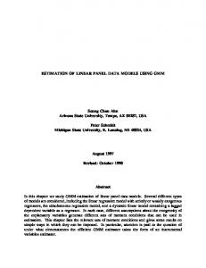
loss. However, from Theorems 3.1 and 3.2 we see that (θˆ1 (X1 , X2 ), θˆ2 (X1 , X2 )) dominates ((α1 − 1)/X1 , (α2 − 1)/X2 ) when we have the restriction θ1 ≥ θ2 , provided that the conditions given in the theorems are satisfied. The condition b2 ≥ α1 given in Theorem 3.2 implies that θˆ2 (x1 , x2 ) = (α2 − 1)/x2 at least in the region x2 > (α2 − 1)x1 /α1 . If the estimator θˆ1 (X1 , X2 ) is to satisfy the order restriction θˆ1 (X1 , X2 ) ≥ θˆ2 (X1 , X2 ) for such an estimator θˆ2 (X1 , X2 ), we need b1 x1 > (α1 − 1)x2 for any (x1 , x2 ) such that (α1 − 1)/x1 < (α2 − 1)/x2 < α1 /x1 . Thus we have b1 ≥ α2 − 1. In this case the region where θˆ1 (x1 , x2 ) is not equal to (α1 − 1)/x1 is different from the one where θˆ2 (x1 , x2 ) is not equal to (α2 − 1)/x2 . This makes it technically difficult to discuss the general problem of improving the UE, c1 (α1 − 1)/X1 + c2 (α2 − 1)/X2 , of c1 θ1 + c2 θ2 for arbitrarily fixed non-negative constants c1 and c2 . We have not succeeded in giving any definite result. Note. Figure 1 shows the regions where θˆ1 (X1 , X2 ) and θˆ2 (X1 , X2 ) differ from UE.
Figure 1. Regions where θˆ1 (X1 , X2 ) and θˆ2 (X1 , X2 ) differ from UE.
4. Numerical results In this section we give some results based on numerical evaluations to illustrate the extent of the risk improvement. We have made numerical evaluations of risk functions of the estimators by first making a variable transformation given by (2.2), and then by performing numerical integration using Mathematica. We first consider the estimation of c1 λ1 + c2 λ2 where c1 and c2 are nonˆ 1 + c2 λ ˆ 2 compared to negative constants. We define the relative risk of MLE c1 λ
344
YUAN-TSUNG CHANG AND NOBUO SHINOZAKI
UE c1 X1 /α1 + c2 X2 /α2 as ˆ 1 + c2 λ ˆ2) R(λ, c1 λ
. X1 X2 R λ, c1 + c2 α1 α2 We have made calculations for 12 cases of (α1 , α2 ): (1, 1), (1, 3), (1, 5), (3, 1), (3, 3), (3, 5), (5, 1), (5, 3), (5, 5), (9, 1), (9, 3) and (9, 5). We have chosen (c1 , c2 ) as (1, 0), (0, 1) and (1, 2), which correspond to the estimation of λ1 , λ2 and ˆ 1 and λ ˆ 2 always dominate UE and that λ1 + 2λ2 respectively. We note that λ ˆ ˆ λ1 + 2λ2 dominates UE except for the cases (α1 , α2 ) = (1, 3) and (1, 5). Without loss of generality we fix λ1 = 1 and have calculated risk estimates for λ2 = 1(1)10. For each choice of (α1 , α2 ) relative risks for three choices of (c1 , c2 ) are shown in ˆ 1 gets smaller when α1 becomes one figure (Fig. 2). We note that relative risk of λ ˆ 2 gets smaller when α1 smaller or α2 larger. On the contrary the relative risk of λ ˆ 2 is quite small in becomes larger or α2 becomes smaller. The relative risk of λ ˆ some cases, but that of λ1 is not small. As a function of λ2 , the minimum seems RR 1.1 1 0.9 0.8 0.7 0.6 0.5 0.4 0.3 RR 1.1 1 0.9 0.8 0.7 0.6 0.5 0.4 0.3 RR 1.1 1 0.9 0.8 0.7 0.6 0.5 0.4 0.3 RR 1.1 1 0.9 0.8 0.7 0.6 0.5 0.4 0.3
α1 =1, α2 =1
1
2
3
4
5
6
7
8
9 10
λ2
RR 1.1 1 0.9 0.8 0.7 0.6 0.5 0.4 0.3
λ2
RR 1.1 1 0.9 0.8 0.7 0.6 0.5 0.4 0.3
λ2
RR 1.1 1 0.9 0.8 0.7 0.6 0.5 0.4 0.3
λ2
RR 1.1 1 0.9 0.8 0.7 0.6 0.5 0.4 0.3
α1 =3, α2 =1
1
2
3
4
5
6
7
8
9 10
α1 =5, α2 =1
1
2
3
4
5
6
7
8
9 10
α1 =9, α2 =1
1
2
3
4
5
6
7
8
9 10
α1 =1, α2 =3
1
2
3
4
5
6
7
8
9 10
λ2
RR 1.1 1 0.9 0.8 0.7 0.6 0.5 0.4 0.3
λ2
RR 1.1 1 0.9 0.8 0.7 0.6 0.5 0.4 0.3
λ2
RR 1.1 1 0.9 0.8 0.7 0.6 0.5 0.4 0.3
λ2
RR 1.1 1 0.9 0.8 0.7 0.6 0.5 0.4 0.3
α1 =3, α2 =3
1
2
3
4
5
6
7
8
9 10
α1 =5, α2 =3
1
2
3
4
5
6
7
8
9 10
α1 =9, α2 =3
1
2
3
4
5
6
7
8
9 10
α1 =1, α2 =5
1
2
3
4
5
6
7
8
9 10
λ2
8
9 10
λ2
8
9 10
λ2
8
9 10
λ2
α1 =3, α2 =5
1
2
3
4
5
6
7
α1 =5, α2 =5
1
2
3
4
5
6
7
α1 =9, α2 =5
1
2
3
4
5
6
7
Figure 2. Relative risks of MLE, dashed line for c1 = 1, c2 = 2, solid line for c1 = 1, c2 = 0, and dotted line for c1 = 0, c2 = 1.
ESTIMATION OF TWO ORDERED GAMMA SCALE PARAMETERS
345
ˆ 1 and λ ˆ 2 . The relative risk of λ ˆ 1 + 2λ ˆ 2 is to be attained when λ2 = λ1 for both λ ˆ 1 and λ ˆ 2 except for some cases where α1 = 1. larger than those of λ Next we consider the estimation of θ1 = 1/λ1 and θ2 = 1/λ2 . We set θˆ1 = max{(α1 −1)X1−1 , (α1 +α2 −1)(X1 +X2 )−1 } and θˆ2 = min{(α2 −1)X2−1 , (α1 + α2 − 1)(X1 + X2 )−1 } and define the relative risk of θˆi compared to (αi − 1)Xi−1 as R(θ, θˆi ) , i = 1, 2. R(θ, (αi − 1)Xi−1 ) We have made calculations for α1 = 2(1)5, 7, 10, and for α2 = 2, 3, 4, 5. Again we fix θ1 = 1 and have calculated risk estimates for θ2 = 1, 1/2, 1/4, 1/8. The relative risks are given in Table 1. We see that risk improvement can be quite substantial in some cases for both θˆ1 and θˆ2 , especially when the value of θ2 is close to that of θ1 . The relative risk of θˆ1 gets smaller when α1 becomes smaller or α2 becomes larger. On the contrary the relative risk of θˆ2 gets smaller when α1 becomes larger or α2 becomes smaller. 5. Concluding remarks In Section 2, the estimation problem of linear functions of ordered scale parameters of two Gamma distributions is discussed under the entropy loss function. We have given a necessary and sufficient condition on two non-negative coefficients for MLE to dominate UE. The same problem has been dealt with under squared error loss functions in Chang and Shinozaki (2002), and a necessary and sufficient condition is given on two coefficients for MLE to dominate UE. A necessary and sufficient condition is also given on coefficients for modified MLE (which we can obtain by replacing αi by αi + 1 in MLE) to dominate �2 i=1 ci xi /(αi + 1). Although negative coefficients are allowed in the case of squared error loss, we restrict analysis to the case with non-negative coefficients and compare the conditions. For the case when c1 > 0 and c2 = 0, similar to the case of the entropy loss function, MLE and modified MLE dominate their competitors under mild conditions. Thus we need only to compare the conditions when c1 ≥ 0 and c2 > 0. Then we notice that three conditions are all of the form c1 /c2 ≤ c(α1 , α2 ), where c(α1 , α2 ) is a constant which depends on α1 and α2 . As is given in Theorem 2.1, c(α1 , α2 ) = α1 /α2 for the entropy loss function. We notice that this is comparable to the result c(α1 , α2 ) = (α1 + 1)/(α2 + 1) when modified MLE is to dominate its competitor under squared error loss. An expression is given for c(α1 , α2 ) in terms of an incomplete Beta function when MLE is to dominate UE under squared error loss in Chang and Shinozaki (2002). The values of c(α1 , α2 ) are numerically evaluated and the results show that they are much smaller than those of α1 /α2 and (α1 + 1)/(α2 + 1). Thus the obtained result for the entropy loss function given in Section 2 is quite similar to the one for the squared error loss function and for modified MLE.
1 0.5 0.25 0.125 1 0.5 0.25 0.125 1 0.5 0.25 0.125 1 0.5 0.25 0.125 1 0.5 0.25 0.125 1 0.5 0.25 0.125
2
10
7
5
4
3
θ2
α1
0.738 0.796 0.894 0.959 0.817 0.866 0.938 0.978 0.858 0.899 0.955 0.985 0.884 0.919 0.965 0.988 0.915 0.942 0.976 0.992 0.939 0.959 0.983 0.995
0.635 0.699 0.805 0.889 0.603 0.676 0.792 0.882 0.585 0.662 0.785 0.879 0.574 0.654 0.781 0.877 0.559 0.644 0.776 0.874 0.548 0.636 0.771 0.872
R(θ, θˆ2 ) � � R θ, α2x−1 2
α2 = 2
R(θ, θˆ1 ) � � R θ, α1x−1 1 0.680 0.768 0.901 0.972 0.760 0.842 0.944 0.987 0.805 0.879 0.961 0.992 0.836 0.901 0.970 0.994 0.875 0.928 0.979 0.996 0.908 0.949 0.986 0.997
R(θ, θˆ1 ) � � R θ, α1x−1 1 0.705 0.792 0.906 0.967 0.661 0.767 0.899 0.966 0.634 0.752 0.896 0.966 0.614 0.742 0.893 0.965 0.590 0.729 0.890 0.965 0.568 0.719 0.887 0.964
R(θ, θˆ2 ) � � R θ, α2x−1 2
α2 = 3
0.643 0.753 0.909 0.981 0.719 0.829 0.952 0.992 0.766 0.868 0.968 0.995 0.798 0.892 0.976 0.997 0.842 0.921 0.984 0.998 0.880 0.943 0.989 0.999
R(θ, θˆ1 ) � � R θ, α1x−1 1 0.756 0.847 0.948 0.988 0.709 0.826 0.946 0.989 0.677 0.813 0.945 0.989 0.654 0.804 0.944 0.989 0.622 0.792 0.943 0.989 0.594 0.782 0.943 0.989
R(θ, θˆ2 ) � � R θ, α2x−1 2
α2 = 4
Table 1. Relative risks of θˆ1 and θˆ2 when θ1 = 1.
0.618 0.745 0.915 0.986 0.689 0.822 0.958 0.995 0.735 0.863 0.973 0.997 0.768 0.888 0.981 0.998 0.814 0.918 0.988 0.999 0.856 0.941 0.992 0.999
0.792 0.881 0.968 0.995 0.746 0.864 0.968 0.996 0.712 0.853 0.969 0.996 0.687 0.846 0.969 0.996 0.652 0.836 0.969 0.996 0.618 0.828 0.969 0.997
R(θ, θˆ2 ) � � R θ, α2x−1 2
α2 = 5 R(θ, θˆ1 ) � � R θ, α1x−1 1
346 YUAN-TSUNG CHANG AND NOBUO SHINOZAKI
ESTIMATION OF TWO ORDERED GAMMA SCALE PARAMETERS
347
Acknowledgements The authors wish to thank an associate editor and the referee for helpful comments. References Barlow, R. E., Bartholomew, D. J., Bremner, J. M. and Brunk, H. D. (1972). Statistical Inference under Order Restrictions, Wiley, New York. Brown, L. D. (1966). On the admissibility of invariant estimators of one or more location parameters, Ann. Math. Statist., 37, 1087–1136. Chang, Y.-T. and Shinozaki, N. (2002). A comparison of restricted and unrestricted estimators in estimating linear functions of ordered scale parameters of two gamma distributions, Ann. Inst. Statist. Math., 54(4), 848–860. Dey, D. K., Ghosh, M. and Srinivasan, C. (1987). Simultaneous estimation of parameters under entropy loss, Journal of Statistical Planning and Inference, 13, 347–363. Fern´ andez, M. A., Rueda, C. and Salvador, B. (2000). Parameter estimation under orthant restrictions, Canad. J. of Statist., 28, 171–181. Hwang, J. T. G. and Peddada, S. D. (1994). Confidence interval estimation subject to order restrictions, Ann. Statist., 22, 67–93. Kaur, A. and Singh, H. (1991). On the estimation of ordered means of two exponential populations, Ann. Inst. Statist. Math., 43, 347–356. Kelly, R. E. (1989). Stochastic reduction of loss in estimating normal means by isotonic regression, Ann. Statist., 17, 937–940. Kubokawa, T. and Saleh, A. K. MD. E. (1994). Estimation of location and scale parameters under order restrictions, J. Statist. Res., 28, 41–51. Kushary, D. and Cohen, A. (1989). Estimating ordered location and scale parameters, Statistics & Decisions, 7, 201–213. Lee, C. I. C. (1981). The quadratic loss of isotonic regression under normality, Ann. Statist., 9, 686–688. Lehmann, E. L. and Casella, G. (1998). Theory of Point Estimation, 2nd ed., Springer. Oono, Y. and Shinozaki, N. (2005). Estimation of two order restricted normal means with unknown and possibly unequal variances, J. Statist. Planning Inference, 131, 349–363. Oono, Y. and Shinozaki, N. (2006a). On a class of improved estimators of variance and estimation under order restriction, J. Statist. Planning Inference, 136, 2584–2605. Oono, Y. and Shinozaki, N. (2006b). Estimation of error variance in ANOVA model and order restricted scale parameters, Ann. Inst. Statist. Math., 58, 739–756. Robertson, T., Wright, F. T. and Dykstra, R. L. (1988). Order Restricted Statistical Inference, Wiley, New York. Rueda, C. and Salvador, B. (1995). Reduction of risk using restricted estimators, Comm. Statist.-Theory and Methods, 24(4), 1011–1022. Shinozaki, N. and Chang, Y.-T. (1999). A comparison of maximum likelihood and best unbiased estimators in the estimation of linear combinations of positive normal means, Statistics & Decisions, 17, 125–136. Silvapulle, M. J. and Sen, P. K. (2004). Constrained Statistical Inference, Wiley, New Jersey. Stein, C. (1959). Admissibility of Pitman’s estimator of a single location parameter, Ann. Math. Statist., 30, 970–979. Van Eeden, C. (2006). Restricted Parameter Space Estimation Problems, Lecture Notes in Statistics 188, Springer. Vijayasree, G., Misra, N. and Singh, H. (1995). Componentwise estimation of ordered parameters of k(≥ 2) exponential populations, Ann. Inst. Statist. Math., 47, 287–307.