This article has been accepted for publication in a future issue of this journal, but has not been fully edited. Content may change prior to final publication. Citation information: DOI 10.1109/ACCESS.2018.2825441, IEEE Access
Date of publication xxxx 00, 0000, date of current version xxxx 00, 0000. Digital Object Identifier 10.1109/ACCESS.2017.Doi Number
Evaluation Models for the Nearest Closer Routing Protocol in Wireless Sensor Networks Ning Cao1,2, Pingzeng Liu3, Guofu Li 4, Ce Zhang5, Shaohua Cao6, Guangsheng Cao1, Maoling Yan3, Brij Bhooshan Gupta7 1
College of Information Engineering, Qingdao Binhai University, Qingdao, China College of Information Technology, Hebei University of Economics and Business, Shijiazhuang, China 3 College of Information Science and Engineering, Shandong Agricultural University, Taian, China 4 College of Communication and Art Design, University of Shanghai for Science and Technology, Shanghai, China 5 School of Computer Science and Technology, Harbin Institute of Technology at Weihai, Weihai, China 6 College of Computer and Communication Engineering, China University of Petroleum, Qingdao, China 7 Department of Computer Engineering, National Institute of Technology Kurukshetra, Haryana, India 2
Corresponding author: Pingzeng Liu (e-mail:
[email protected]).
This work was supported by Grant Shandong Education Department J16LN73, Shandong independent innovation and achievements transformation project (2014ZZCX07106), and Natural Science Foundation of China (No. 61572022).
ABSTRACT Wireless sensor networks have been pushed to the forefront in the past decade, owing to the advert of the Internet of Things. Our research suggests that the Reliability and Lifetime performance of a typical application in wireless sensor networks depend crucially on a set of parameters. In this paper, we implemented our experiments on the Nearest Closer protocol with the J-Sim simulation tool. We then analyze the closure relationships among the Density, Reliability and Lifetime, and reveal the trade-off among them based on our analysis on the experiment results. Next, we propose five intelligent evaluation models that are applicable to such situations. Our research allows the wireless sensor network users to predict the significant evaluation parameters directly from the settings while costly simulations are no longer necessary. INDEX TERMS Evaluation Model; Nearest Closer; Routing Protocol
I. INTRODUCTION
The next generation networks have the potential to offer heterogeneous connectivity, especially for the IoT systems. When the transmission speed reaches 10Gbps, 10 to 100 times faster than that of the 4G networks, massive types of wireless communications demand can be fulfilled [1-3]. IoT systems must allow things to be inexpensive, highly power efficient, ubiquitous, safe and reliable [4-6]. Research related to sensors is a significant research point for IoT. The research of Wireless Sensor Networks (WSNs) is a subset research area of IoT. The sensors should be assigned with a routing protocol, so that instead of transmitting data directly to the end-user, they choose to transmit their data via a number of other sensors subject to the condition that the data will eventually arrive at the end-user (multi-hop protocol). 5G can provide a reliable backhaul infrastructure for many IoT systems. In addition, the communication security [7-9] and security of sensor networks [10-13] are also very important. It is necessary to prevent the monitoring data from being stolen and to obtain forged monitoring information.
The main problems in the primary research area of WSNs are conserving sensor energy [14-17] and improving data accuracy [18-19]. For instance, Raghunathan et al. discuss several key factors, including architecture and protocols, which are related to energy-efficient design of sensor nodes in a WSN [20-22]. The properties of data security and energy consumptions in wireless networks are highly depend on the physical neighborhood and the transmission power, which makes previous theories for wired networks no longer viable. Although many of the researches realize that energy consumption and reliability are the important parameters for a WSN, which are also influenced by the features of the network, there have been very few research works focus on the tradeoff between the important factors of reliability, lifetime, and node density empirical. They also haven’t proposed effective evaluation models among these parameters. In [23], Maity & Gupta considered a randomly distributed wireless sensor network covering a large area. They wished to find an estimate for the number of nodes required with the minimum critical communication distance to ensure network
VOLUME XX, 2017
2169-3536 (c) 2018 IEEE. Translations and content mining are permitted for academic research only. Personal use is also permitted, but republication/redistribution requires IEEE permission. See http://www.ieee.org/publications_standards/publications/rights/index.html for more information.
This article has been accepted for publication in a future issue of this journal, but has not been fully edited. Content may change prior to final publication. Citation information: DOI 10.1109/ACCESS.2018.2825441, IEEE Access
connectivity and stability. Using results from graph theory certain mathematical formula-based algorithms already existed for a relatively small number of sensors; however, the authors proposed a new formula based on mathematical simulation, which minimized the inter-node critical radius prediction for a large number of nodes. They chose MATLAB as their simulation tool and constructed a regression equation between the radius and number of nodes. The theoretical model provided better results if the number of nodes is less than 250, but their regression equation provided smaller answers for the radius to preserve connectivity for larger numbers of nodes. In our research, we will combine three parameters together and propose the evaluation model among these parameters. The model can also provide good results even if the number of nodes is greater than 250. This research seeks to develop some evaluation models, which will serve to inform the organization of a high efficiency wireless sensor network without prior use of simulations. Such mathematical models will avoid the necessity to undertake simulations for the deployment of sensor nodes resulting in a saving of both time and money. In this paper, we choose the Nearest Closer protocol as a typical routing protocol for location-based routing protocols [24-27]. After obtaining several useful results via simulations, several evaluation models based on the Nearest Closer routing protocol [28] in wireless sensor networks will be proposed. II. MATERIALS AND METHODS A.
SIMULATION TOOLS
Before the real deployment of sensors to the real area, to do simulation is really significant. From the simulation results, users can conclude how the routing protocols work. After comparisons of simulation results, users can select the most suitable routing protocol for their applications. There exist several simulation tools, such as: NS-2 [29], Omnet++ [30], TOSSIM [31], J-Sim [32-33]. J-Sim will be selected as the simulation tool for this paper. The reason can be explained as follows: J-Sim is an open-source simulation tool. J-Sim has provided a strong energy model to the users. J-Sim has a good user interface and is convenient for the users to invoke the existing methods. J-Sim is a Java-based simulation tool, it will be possible to combine the energy model with the Java-based sensor’s energy model in future design. The authors of J-Sim have performed detailed performance comparisons in simulating several typical WSN scenarios in JSim and NS-2. The simulation results indicate J-Sim and NS2 incur comparable execution time, but the memory allocated to carry out simulation in J-Sim is at least two orders of magnitude lower than that in NS-2. As a result, while NS-2 often suffers from out-of-memory exceptions and was unable to carry out large-scale WSN simulations, the proposed WSN framework in J-Sim exhibits good scalability.
J-Sim models are easily reusable, so users can combine the components in the framework freely. B.
NEAREST CLOSER PROTOCOL
The Nearest Closer protocol is both a typical location-based routing protocol and a multi-hop routing protocol. Consequently, this work has implemented the protocol in JSim as an example. To implement this protocol each node has to know its own position, the position of its neighbors within its transmission range, and the position of the sink node. The main idea in the Nearest Closer protocol is that the transmitter sensor will transmit to its nearest neighbor that is closer to the sink node (the distance between the neighbor and the sink node is less than the distance between the sensor node and the sink node; choose the nearest neighbor from the sensor node). Slotted ALOHA protocol has been selected as the MAC layer protocol. Slotted ALOHA is a type of TDMA transmission system and it improves contention management through the use of beaconing. Slotted ALOHA can make a single active sensor nearly continuously transmit at full channel rate, thus better results can be obtained for the Nearest Closer protocol. C. REASON TO SELECT NEAREST CLOSER PROTOCOL
The location-based routing protocols, of which there are a large number, but difficult to be implemented in J-Sim Greedy Perimeter Stateless Routing (GPSR) essentially allows backtracking if a dead end is reached, so within any implementation program for GPSR and other similar routing protocols there must be a large number of nested conditional statements of the ‘IF’ and ‘THEN’ form. This means that the behavior of the protocol can fundamentally change during a simulation depending on the geographical and/or power status of the network, so that trends in results obtained from simulations using such protocols will be difficult (if not impossible) to analyze. The choice in this thesis, to avoid such conditionality and the apparent complexity of any resultant mathematical model, came down to Nearest with Forward Progress (NFP) or Nearest Closer (NC) for the work. The routes in NFP along which sensors transmit data to the sink node will be very jagged (with lots of ‘ups’ and ‘downs’) compared to those in NC by definition. Thus NC presents, at face value at least, a more sensible approach to transmitting data from a sensor to the sink node and hence our choice of it as a representative for location-based protocols. D.
EXPERIMENTAL SET-UP
The simulated area for the following experiments is defined as a 10 meter by 10 meter square. All the sensor nodes are randomly deployed. The routing protocol is the Nearest Closer. The sink node is in the middle of this simulation area. There exists a fixed target node in each simulation experiment, and this target node will generate a stimulus every one second. All the sensors are active at the start of the simulation (For the NC
VOLUME XX, 2017
2169-3536 (c) 2018 IEEE. Translations and content mining are permitted for academic research only. Personal use is also permitted, but republication/redistribution requires IEEE permission. See http://www.ieee.org/publications_standards/publications/rights/index.html for more information.
This article has been accepted for publication in a future issue of this journal, but has not been fully edited. Content may change prior to final publication. Citation information: DOI 10.1109/ACCESS.2018.2825441, IEEE Access
protocol, the sensor nodes can only transmit its data to the nearest neighbor sensor as the routing map will be generated before data transmission.). The simulation time is enough for obtaining data in each separate experiment. All the points (in the figures) in this paper are the average value from 5 separate experiments. In each experiment the sensors are static once placed, and the sensor nodes are re-positioned randomly for the 5 experiments. The Network Lifetime will be measured in seconds. The maximum simulation time for all experiments in this paper is 100,000 seconds. III.
RESULTS
A.
EVALUATION PARAMETERS
a)
RELIABILITY
FIGURE1. Density, Reliability Relationship for NC.
This paper bases its experiment on the concept of Reliability, which is defined as: the number of packets received by the sink node
Reliability =
the number of packets sent directly to the sink node
b)
(1)
LIFETIME
Network Lifetime has various definitions. Some researchers may select the time when the all the sensors run out their energy to define the Lifetime, however, if the key sensors in this WSN are dead, this sensor network will never continue to work anymore. So this is not a good choice for the definition of Lifetime. Some researchers may select the time when the first sensor is dead to define the parameter of Lifetime. But this is not a suitable moment for Lifetime as the sensor network may work well. In this paper, we will select the timepoint when the last packet sent from sensors is received by the sink node to define the Lifetime. c)
In Figure 1, we observe a clear relationship between the number of sensors and the Reliability, which, in this application, increased as the number of sensors increased to 40, when it reached its highest value. It then essentially decreased as the number of sensors increased from 40 to 300, when it reached its lowest value. This may be explained by observing that: as the Density increases, more sensors will join the data transmission process and consequently communication among the sensors will become more and more complex. So, dropped data due to data collision and latency cannot be ignored. Consequently, it is reasonable to expect the Reliability to decrease with the Density.
DENSITY
In a fixed area, the number of sensors deployed can be used to denote the Density. B.
RESULTS AND ANALYSIS
A series of experiments [34] was carried out with the number of sensors starting at 10, and increasing in increments of 10 up to 300 sensors. The transmission radius for each sensor was fixed at 15 meters as this is large enough to transmit data anywhere within the square.
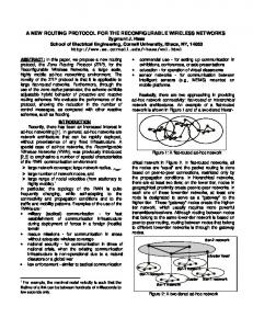
FIGURE 2. Density, Lifetime Relationship for NC.
In Figure 2, the Lifetime meets its minimum value when the number of sensors equals to 220, whereas the highest value of the Lifetime occurred when there were 10 sensors. In the NC protocol, sending a packet to the sink node will require each sensor to transmit its data down transmission trees to the nearest sensors to the sink node. These nearest sensors (only about two or three) will be receiving all the data in the network and transmitting it all to the sink node, using a large amount of energy. Thus, a NC network will generally die fairly rapidly from the sink node outwards. In Figure 1, note that when the number of sensors equals 40, the Reliability was 93.64%, its highest level, but with this
VOLUME XX, 2017
2169-3536 (c) 2018 IEEE. Translations and content mining are permitted for academic research only. Personal use is also permitted, but republication/redistribution requires IEEE permission. See http://www.ieee.org/publications_standards/publications/rights/index.html for more information.
This article has been accepted for publication in a future issue of this journal, but has not been fully edited. Content may change prior to final publication. Citation information: DOI 10.1109/ACCESS.2018.2825441, IEEE Access
number the Lifetime is fairly short. This illustrates that it is possible for users to choose an optimum Density value for this application depending on the Reliability and Lifetime required. IV. BASE EVALUATION MODELS A.
50
2.531
60
2.550
70
2.542
80
2.534
90
2.553
100
2.549
110
2.568
120
2.578
130
2.555
140
2.543
150
2.574
160
2.550
170
2.557
180
2.552
190
2.575
200
2.582
210
2.574
220
2.600
230
2.571
240
2.573
250
2.569
260
2.551
270
2.575
280
2.543
290
2.563
300
2.562
LIFETIME MODEL
The energy requirement of a routing task can be largely approximated by the hop count, under which circumstance we assume a constant metric per hop. However, if nodes can adjust their transmission power (knowing the location of their neighbors) the constant metric can be replaced by a power metric u ( d ) = e + da (or some variation of this) for some constant value of a and e that depend on the distance d between nodes. The value of e , which includes energy loss due to start up, collisions, retransmissions, and acknowledgements, is relatively significant, and protocols using any kind of periodic hello messages are extremely energy inefficient. Our motivation of proposing the NC protocol is based on the consideration that the average energy consumption of a sensor for data to its nearest neighbor can be calculated by a simple formulae w ( s ) E d 2 , in which E d 2 is the expectation of the squared distance between the sensors, and w ( s ) is the average number (weight) of packets of data to be sent to its nearest neighbor. In the NC protocol one possible parameter that could affect the Lifetime is the number of paths or trees formed by the sensors. This is not the case as demonstrated by the following experiments, which are of independent interest. Using J-Sim it is difficult to extract the paths that sensors transmit along to the sink node. For this reason, a program was written in the algebraic software package Magma to not only compute the individual paths, but to marry them together in order to form the initial distinct trees. During the Lifetime of the network various sensors will die, normally from the center outwards, and new trees will be formed (The sink node is in the middle. Tree roots are close to the sink node and they will die quickly as they do receive and transmit data frequently. In this paper, all the common sensors are randomly deployed and have the same power.). The mean number of trees is shown in Table I. The effect of randomly placed sensors in each experiment can be ignored as the value was averaged from the results of 1000 experiments.
( )
( )
TABLE I. MEAN NUMBER OF TREES
No. of Sensors
Trees
10
2.537
20
2.527
30
2.561
40
2.559
According to Table I, we conclude that the average number of trees is independent of the number of sensors, and thus can be discounted as having any effect on the Reliability or Lifetime. The reason that two or three trees may appear on average can be fully explained by considering the diagram below. In the case of 300 sensors, the number of trees with frequencies was one with frequency 1, two with frequency 42, three with frequency 53 and four with frequency 3. The distributions for two trees took various values from (299, 1) to (152, 148). For the cases of two trees the average length of the
VOLUME XX, 2017
2169-3536 (c) 2018 IEEE. Translations and content mining are permitted for academic research only. Personal use is also permitted, but republication/redistribution requires IEEE permission. See http://www.ieee.org/publications_standards/publications/rights/index.html for more information.
This article has been accepted for publication in a future issue of this journal, but has not been fully edited. Content may change prior to final publication. Citation information: DOI 10.1109/ACCESS.2018.2825441, IEEE Access
two trees for 10 sensors was 6.69 and 3.31 with a sample standard deviation of 1.199. The ratio between these average lengths is 2.02. For 40 sensors the corresponding figures are 26.667 and 13.333 with a sample standard deviation of 4.646. The ratio between these average lengths is 2. For 300 sensors the corresponding figures are 213.929 and 86.071 with a sample std. value of 39.38. The ratio between these average lengths is 2.49. The reason for using the average tree length as a test statistic is that it can be generalized to more than two trees. In the latter part of this paper it is assumed that the sensors are equally distributed amongst the trees. The results above indicate in the two-tree case that the ratio between the average lengths of the trees is about 2 or 2.5 to 1. The reason for this may be that the shape of the square influences the sensors into one large and one small tree, this merits further investigation from a mathematical or statistical perspective. For the NC protocol the relation ‘is the closest neighbor to’ is not symmetric. In Figure 3, B might be the closest neighbor to A, but without A being the closest neighbor to B. Thus, for this protocol it is necessary to find the closest neighbor to a sensor A, but with the stipulation that the neighbor is closer to the sink node than A. It is also the case that the sink node could be the closest neighbor to A, but the sink node is a fixed point and therefore does not fit in with the assumption that this work is dealing with a random distribution of sensors. The second column of Table II lists the expectation of the distance d between a sensor node and its closest neighbor that should be closer to the sink, and the third column shows the expectation of the squared distance d 2 . Finally, the fourth column shows the average weight of the sensors, where each branch in the various trees count as weight one. This is a measure of the number of packets of data an average sensor has to transmit to its nearest neighbor, and it is also the average number of hops from the sensors to the sink node. The results of these simulations are tabulated in Table II (In Table II, E ( d ) denotes the expectation of the distance between sensors, E d 2 denotes the expectation of the squared distance between sensors, and w ( s ) denotes the average number (weight) of packets of data to be sent to its nearest neighbor.) Note that, for those sensors whose nearest neighbor is the sink node that the distribution of the distance and squared distance to the sink node is slightly different to those between sensors, and the averages are always slightly higher than those given in Table II, with the exception of the 10 sensor case when there is a significant difference. We induce two conclusions from this table. First, the value of w ( s ) E ( d ) is nearly constant which varies between 5.16 and 5.45, and is a measure of the average distance from a sensor to the sink node measured along the hop path. Second, the value of w ( s ) E d 2 decreases when the number of sensors growth, which shows that the energy expended by a sensor in receiving and sending received packets to its nearest neighbor decreases when the number of sensors increases. It also represents a measure of the average amount of energy
( )
( )
required to transmit one packet of data to the sink node. Two theories are proposed to explain why the Lifetime decreases as the number of sensors goes up.
FIGURE 3. Typical Tree Zones.
TABLE II EXPECTED DISTANCES AND WEIGHTS, VARIABLE SENSORS.
Sensors
𝐸(𝑑)
𝐸(𝑑 2 )
𝑤(𝑠)
10
2.1945
6.0533
2.3526
20
1.5985
3.2761
3.3421
30
1.3223
2.2444
4.0821
40
1.1512
1.7023
4.7152
50
1.0264
1.3535
5.2218
60
0.9402
1.1350
5.7941
70
0.8672
0.9679
6.2249
80
0.8104
0.8450
6.6531
90
0.7657
0.7545
7.0685
100
0.7256
0.6759
7.4110
110
0.6926
0.6155
7.7859
120
0.6618
0.5634
8.1589
130
0.6360
0.5200
8.4701
140
0.6124
0.4817
8.7956
150
0.5910
0.4485
9.0999
160
0.5724
0.4210
9.4502
170
0.5553
0.3957
9.7218
180
0.5394
0.3734
9.9967
VOLUME XX, 2017
2169-3536 (c) 2018 IEEE. Translations and content mining are permitted for academic research only. Personal use is also permitted, but republication/redistribution requires IEEE permission. See http://www.ieee.org/publications_standards/publications/rights/index.html for more information.
This article has been accepted for publication in a future issue of this journal, but has not been fully edited. Content may change prior to final publication. Citation information: DOI 10.1109/ACCESS.2018.2825441, IEEE Access
E T K (1- l ( n )) ´ 223 + l (n) ´ nE( d)
190
0.5240
0.3525
10.3059
200
0.5108
0.3346
10.5684
210
0.4983
0.3183
10.7823
220
0.4874
0.3046
11.0709
230
0.4759
0.2904
11.2847
240
0.4658
0.2785
11.5108
1.1438571428571 - 0.01501071428514 x,
250
0.4562
0.2670
11.8269
for 10 £ x £ 70,
260
0.4466
0.2559
12.0056
270
0.4393
0.2475
12.2536
280
0.4308
0.2378
12.4573
290
0.4231
0.2296
12.7054
300
0.4160
0.2216
12.9399
( ) 2
In general, the Lifetime can be modelled by considering only the roots of the forest, which normally consists of just two or three trees. If there exists just one tree, which is an interesting case for a small number of sensors, the system should run until the only root sensor dies naturally, when the system might interpret the death as a transmission break or the next sensor(s) out will take over the role of the root(s). In either case, the Lifetime is expected to be much longer for just one tree. The basic model constructed here is of the form
E (T ) K nE d 2
( )
(2)
, where n is the number of sensors, K is the initial energy of a sensor and E ( T ) is the expected number of trees. Here n / E(T ) represents the average weight per tree and since E ( T ) is nearly constant, the model should roughly resemble the curve 1/ n . Particularly, this model assumes that the sensors are evenly distributed amongst the trees and is ignorant of data build-up, so it can be deemed as an upper bound for the Lifetime if the system runs at full capacity. The implication is that the Lifetime decreases monotonically as the number of sensors increases; however, this basic model assumes that the system runs at full capacity from the start and ignores idle slots in the slotted ALOHA design. Thus there is a base value below which the Lifetime will not fall, as the system will behave in a manner akin to a sparser system during its initial phase and there will furthermore always be a number of idle slots. This base value will be taken to be the smallest Lifetime value of 223 that occurs when n = 220 . So the revised model is:
(3)
, where l ( n ) is a proportionality measure with l ( 220 ) = 0 . Now from the Lifetime data l ( n ) will be very close to 0 if n ³120 . Setting l (10 ) = 1 yields the value K = 16,750 . The parameter l ( x ) can be piecewise approximated by (4)
and
0.3954 - 0.0029514285714286 x,
(5)
for 80 £ x £ 130
by fitting straight lines through the given values. An alternative that will yield better local approximations is to interpolate between the known values of λ. Thus, if n≤x