Evolving a Hybrid K-Means Clustering Algorithm ... - Semantic Scholar

IJCSI International Journal of Computer Science Issues, Volume 12, Issue 1, No 1, January 2015 ISSN (Print): 1694-0814 | ISSN (Online): 1694-0784 www.IJCSI.org

23

Evolving a Hybrid K-Means Clustering Algorithm for Wireless Sensor Network Using PSO and GAs Alaa Sheta1 and Basma Solaiman 2 1

Software Engineering Department, College of Science and Information Technology Zarqa University, Zarqa, Jordan 2

Computer Science Department, College of Computer Science and Information Technology, Sudan University of Science and Technology (SUST) Khartoum, Sudan

Abstract Wireless Sensor Networks (WSN) became an essential component in many real-life applications such as military, smart energy, commercial, health and many others. However, WSN still suffer many problems related to energy consumption. Clustering found to be an effective technique to solve the energy consumption problem for WSN by avoiding long distance communication. In this paper, we explore our initial idea on developing a hybrid clustering algorithm which has two folds 1) Use the K-Means unsupervised learning algorithms to select the sensors belonging to each cluster using an arbitrary number of clusters 2) Use Particle Swarm Optimization (PSO) and Genetic Algorithms (GAs) separately to select the best CHs. We name these two algorithms as KPSO and KGAs. The developed hybrid algorithms are tested over number of experiments with various layouts. KPSO provided better results compared to the KGAs. Keywords: Wireless Sensor Network, Clustering Algorithms, KMeans, Particle Swarm Optimization, Genetic Algorithms.

sensed data locally, and then send the data to a base station for further processing through wireless communication, mostly radio frequency (RF). Each node is equipped with a battery that has limited lifetime. Most of the node’s energy is consumed during communication [6]. The consumed energy during communication is affected exponentially by the distance between the communicating nodes; the more communication distance between two nodes the more energy consumed. WSNs are very sensitive to energy consumption and its performance depends on the network lifetime. The network lifetime is an indication of the network degradation; the death of one node is soon succeeded by death of others and nodes isolation. Therefore, managing energy consumption is a vital task in WSN performance.

1. Introduction Wireless networking is an emerging technology that allows users to access information and services electronically, regardless of their geographic position. WSNs are deployed, uniformly or randomly, in land, underground and underwater [1]. WSN was first inspired by the US military for enemy surveillance and object tracking [2]. Recently, it is applied to diverse civil applications as: environment monitoring [3] and environmental disaster detection [4]. Nowadays, hundreds or thousands of heterogeneous reliable and low cost micro sensors [5] are deployed over a geographical area of interest, and communicate together forming a wireless sensor network. WSNs are estimated to work for months and years according to the application. Wireless sensors (nodes) in the network sense external data from the surrounding environment, process the

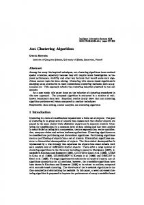
Fig. 1: Clustered WSN

Clustering is a very common technique which is most likely to be used to decrease the communication distance and preserve nodes energies. Clustering partition the nodes into groups called clusters. In each cluster, a node is chosen to be the cluster head (CH). The CH’s function is to collect data messages from the nodes belonging to its cluster. Then the CH sends a message containing

2015 International Journal of Computer Science Issues


aggregated data to the base station. In Figure 1, we show a simple example of a clustered WSN. Clustering technology has many advantages which can be summarized as follows: 

minimizes communication overhead



enhances resource use. For example, non-neighbor clusters can use the same communication frequency.



scalability; nodes can join or leave the group without affecting the entire network.

In this paper, we propose a hybrid K-means PSO/GAs clustering algorithm. Both the KPSO and KGAs shall be used to define the sensors belonging to each cluster and the best CHs. This paper is organized as follows: WSN components are described in Section 2. Both the GAs and PSO algorithms are briefly described in Sections 3 and 4, respectively. The K-Means clustering algorithm is presented in Section 5. The problem Hybrid KMean clustering algorithm is presented in Section 6. In Section 7, we described the characteristics of the developed WSN Clustering Toolbox. The setup for WSN simulation along with the assumption made for our simulator is presented in Section 8. The developed results are shown in Section 9. Investigations on the reliability of our developed models with the variation in the number of sensors, the sensor energy and the location of the base station, were explored in Section 10.

2. Components of WSN? WSN consists of spatially distributed autonomous sensor nodes [7]. The sensor nodes investigate the surrounding environment and send the recorded data to a highly computed station, called sink. The sink is responsible for collecting and processing the data received from the nodes. The wireless sensor node consists of [8]:  Sensing unit: sensor(s) that measures data from the surrounding. 

Processing unit: processes the measured data and data received from neighbor nodes.



Transceiver: responsible for sending and receiving data using communication media (most commonly radio waves).



Battery: un-rechargeable limited battery.

and

un-replaceable

A survey on the use of various search algorithms to solve clustering problems of WSN along with many applications is presented in [9]. Moreover, Clustering

24

using Fuzzy logic was also investigated in [10, 11].

3. Genetic Algorithms Genetic algorithms (GAs) are adaptive search algorithm which were presented by J. Holland [12], and extensively studied by Goldberg [13, 14], DeJong [15, 16, 17], and others. GAs successfully handled many areas of applications and was able to solve a wide variety of difficult numerical optimization problems. GAs requires no gradient information and is much less likely to get trapped in local minima on multi-modal search spaces. GAs found to be quite insensitive to the presence of noise [18]. The pseudo code of the GAs method [13, 14] is shown in Algorithm 1. Using GAs, the problem is encoded into chromosomes representing possible solutions. A fitness function is used to investigate the quality of each individual in the population. The individuals in a population undergo crossover and mutation to produce the next generation. Crossover makes new solution by concatenating parts of two selected chromosomes. Mutation is useful in overcoming local-minima entrapment. The repeated process of crossover and mutation eventually leads to the best solution. Algorithm 1: Basic steps of GAs 1 begin GAs 2 g = 0 generation counter 3 Initialize population 4 Compute fitness for population P (g) 5 While (Terminating condition is not reached) do 6 g = g +1 7 Select P (g) from P (g − 1) 8 Crossover P (g) 9 Mutate P (g) 10 Evaluate P (g) 11 end while 12 end GA

4. Particle Swarm Optimization Particle Swarm Optimization (PSO) is a population based search algorithm, with particles representing possible solutions. The particles move in the search space, communicate with their neighborhoods, and use a fitness function to identify their next location in the search space. The PSO particles iteratively update their velocities and positions until they converge into a possible optimal solution. The basic PSO algorithm is shown in Algorithm 2. An efficient energy management of the WSNs based PSO was provided in [19].



Algorithm 2: Basic steps of PSO 1 begin PSO 2 Randomly initialize the position and velocity of 3 the particles: Xi(0) and Vi(0) 4 While (Terminating condition is not reached) do 5 for i = 1 to number of particles 6 Evaluate the fitness:= f(Xi) 7 Update pi and gi 8 Update velocity of the particle Vi 9 Update position of the particle Xi 10 Evaluate the population fitness 11 Next for 12 end while 13 end PSO

6. Hybrid K-means Clustering Algorithm WSN clustering algorithm for n sensors will have to examine solutions to find the optimal clustering layout. We propose two Hybrid K-means clustering algorithms to solve for clustering WSN in order to increase the network lifetime. They are: KPSO and KGA.

5. K-Means Clustering K-Means clustering is one of the simplest unsupervised learning algorithms. It is heuristic in nature, and proved to be effective in determining clusters of spherical shapes [20]. It was applied to partition a network into number of clusters [21, 22, 23]. It classifies a given data set into a predefined number of clusters, k. Its main idea is to define k centroids, one for each cluster. In [24], the authors compared between two developed K-Means clustering models for WSN: centralized and distributed. The algorithm for obtaining the centroid aims at minimizing an objective cost function which is a squared error function [23]. The objective function can be simply defined as: ∑

∑

‖

‖

25

(1)

where ‖ ‖ is the Euclidean distance measure between a data point and the cluster center . D is an indicator of the distance of the n data points from their respective cluster centers. There are different matrices that can be used other than Euclidean distance [25, 26]. In the following steps we summarize how K- means work. 1) Arbitrarily choose k points known as cluster centers. k is also defined as the number of clusters anticipated. 2) Calculate the distance between each sensor and the cluster centers, and allocate each sensor to the closest cluster center. 3) Calculate the new cluster center by calculating the mean distance between each cluster center and all sensors in its range. 4) With the new cluster centers, repeat Step 2. If the allocated cluster center changed for the sensors in a cluster, repeat step 3 else stop the process.



Phase 1: We apply the K-means algorithm to divide the network into k clusters. k is arbitrary selected.



Phase 2: PSO/GAs algorithms goal is to select the best CH within each cluster obtained by the K-Means clustering algorithms.



Phase 3: We evaluate the resulting cluster layout.

Our proposed hybrid algorithm decreases computational effort. In our algorithm, the search space will be reduced to about

solutions for each cluster.

6.1 Phase 1: K-Means Clustering In our proposed algorithm, the K-means clustering algorithm is applied to divide the network to a predefined number of clusters, k. The base station will select k nodes as CHs, then each node joins its nearest CH. Next, a new CH is chosen as the middle of the cluster. These steps are repeated until no new CH is selected. The distance between two nodes n1, n2 is computed based on the following Euclidean distance calculation: (

)

√(

)

(

)

( )

x and y are the node’s x-coordinate and y-coordinate respectively. This phase will divide the network to disjoint clusters. The base station will save information about each cluster: sensor node ID and location, and CH identification.

6.2. Phase 2: CH Selection Both PSO and GAs algorithms were applied separately to select the optimal cluster head from each cluster obtained by the K-means phase. For instance, if the K-means algorithm partitioned n nodes to 2 clusters with a, and b nodes, respectively, then the PSO/GAs algorithms will select two cluster heads from the a nodes and the b nodes respectively.  Encoding the Problem: The PSO particle structure and GA chromosome structure are identical, as shown below. CH1


CH2

......

CH k


It represents an array containing the indices of each node, for every cluster, elected as CH. Knowing that Kmeans has divided the WSN into k clusters, the PSO particle and GA chromosome sizes are fixed. 

Fitness Function: Our proposed fitness function is used for both GA and PSO. It is a representation of the number of transmissions a CH performs. Equation 3 shows the fitness function. Ei represents the CH’s actual energy and di is the Euclidean distance between the cluster head and the base station. The value of do is 87 m [27]. The algorithm is aimed to maximize CH transmissions. ∑ ( ) ∑ {

6.3. Phase 3: Model Evaluation This phase simulates the energy consumed by every node in the network. The equations adopted calculate the Dissipated Energy (DE) in sensing and processing data plus transmitting a 1-bit message to short and long distances respectively. The DE by a CH ( ) is given in Equation 4, while Equation 5 shows the DE by a nonCH ( ) node. This phase also counts for dead and remaining alive nodes

{

(4)

{

(5)

where • ni is the number of nodes belonging to CHi , •

dtoBS is the Euclidean distance between the CH and the base station,

• dtoCH is the Euclidean distance between the node and its CH, • Ee = 50nj, 0.0013pj/m4.

= 5nj,

= 10pj/m2, and

=

26

7. Developed WSN Clustering Toolbox We implemented a WSN Clustering Aided Toolbox (WSNCAT) to simulate our proposed algorithm. Figure 2 shows the graphical user interface (GUI) of the developed toolbox using MATLAB software. The graph on the left shows the developed cluster layout. The graphs in the middle and on the right show the total remaining energy and the total number of alive nodes respectively. Figure 3 shows the block diagram of Our developed MATLAB toolbox. It consists of the following components:  WSN Data Module In this module the user specifies the length and width of the geographic data, the location of the base station and the number of sensor nodes. The user also decides whether the nodes’ data are generated randomly, loaded from a M ATLAB workspace, or entered manually.  Clustering Data Module In this module, the user decides which technique is used: PSO, or GA. Our fitness function presented in Equation 3 is used by default. Other fitness functions are also embedded in the toolbox. The user can specify the number of clusters. In case the number of clusters is not specified, the toolbox tests the nodes layout and calculates for the best number of clusters based on K-means algorithm.  Clustering Module This module is triggered after all the simulation data are saved form the above mentioned modules. It runs our proposed hybrid algorithm. The graph on the left of the GUI shows the WSN clustering layout resulted from running the hybrid algorithm  Simulation Module This module is triggered by the clustering module. In this module, we developed our own simulator to evaluate our proposed clustering algorithm. Our developed simulator reports the WSN data during each transmission. It calculates the total consumed energy for every sensor node and the total alive nodes based on the radio model described in [28] and modeled in Section 6.3.

8. Setup for WSN Simulation 8.1 Assumptions We assumed fixed number of static nodes that have initial energy, and are randomly deployed in a two dimensional geographical area. A highly computed base station is located within or far from the node’s geographic area. It



27

Fig. 2: WSN-CAT Toolbox GUI

Fig. 3: WSN-CAT Toolbox Operational Structure

also has information about the nodes location. It is assumed that there are no communication problems between the nodes and the base station, and also between the nodes and their CHs. Moreover, communication is assumed to be established over time. Within each cluster, each pair of sensor nodes is guaranteed to be within the effective transmission range. So each two nodes in the cluster can communicate with each other directly. In a transmission cycle, each node sends a single data message to its CH. Then the CH aggregates the received data into one message. The nodes and the base station are assumed to communicate using the RF model. Finally, the CH sends the aggregated message to the base station.

8.2 Selecting the Number of Clusters We made a pretest to discover the number of clusters

producing the minimum communication distance. Figure 4 shows the total communication distance versus the number of clusters. Table 1 lists the values of the parameters adopted in our experiment. Table 2 lists the parameters of the PSO model used. Table 3 lists the parameters of the GA model used. Table 1: WSN simulation parameters

Parameter Field size Number of sensor nodes

Value 100 × 100 m2 100

Energy of sensor nodes Base Station location Number of clusters Size of message

80% have 2J ; 20% have 5J (0,0) 9 4000 bits



28

Fig.4. Communication distance vs. number of clusters Table 2: PSO simulation parameters

Parameter PSO model Inertia weight ψ1 ψ2 No. of particles

Value TVAC [29] [0.1:0.9] [0.5:2.5] [0.5:2.5] {20,40,60,80}

Fig. 5. Total remaining energy vs. number of transmissions

Table 3: GA simulation parameters

Parameter Selection Prob. Crossover Type No. of Crossovers Mutation Type No. of Mutations Population Size

Value 0.08 arithmetic crossover 2 non-uniform mutation 2 {20,40,60,80}

9. Experimental Results In this section, the results of applying our hybrid algorithms - for the WSN stated in Table 1- are described. The total remaining energy based on the two algorithms studied in this research (i.e. KPSO and KGA algorithms) are presented in Figure 5. Figure 6 shows the number of alive nodes versus the number of transmissions. Both KPSO and KGA algorithms preserve the same total energy during the first half of the network lifetime. In the second half, KPSO consumes more energy than KGA. However, KPSO performs more transmissions than KGA. In Figure 7, we show the developed cluster layout for the K-means algorithm alone, the layout after applying the KPSO algorithm, and the clusters layout formed by the KGA algorithm. The nodes marked with ’red star’ are those having high energy. The cluster head selected by Kmeans algorithm is the center of the cluster. However, the CHs selected by our KPSO algorithm, and KGA algorithm is not necessarily the center of the cluster. The proposed fitness function selects the cluster head that can survive for maximum number of transmissions. Figure 8 show the GAs and PSO fitness conversion. The graph shows that PSO converges to higher (i.e. better) fitness than GAs, with higher number of generations.

Fig. 6. Total no. of alive sensor nodes vs. number of transmissions

Fig. 8. PSO and GA fitness conversion graphs

Table 4 shows the various simulated number of transmissions along with the number of alive sensor nodes. The simulated results show that KPSO performs more transmissions than KGA. The number of transmissions performed by a given number of alive sensors using the proposed KPSO algorithm was improved than using



29

Fig.7. (a) K-means clusters (b) KPSO clusters (c) KGA clusters

the KGA algorithm. For example, if we consider the network lifetime as when 10% of the sensors die: the number of KPSO transmissions is more than KGA transmissions by about of 30%; i.e. we can say that the WSN lifetime using KPSO is more than WSN lifetime using KGA. Table 4: Simulated number of transmissions

Number of alive sensor nodes 100 90 80 70 60 50 40 30 20 10

Simulated transmissions KGA KPSO 555 604 2732 3518 3614 4714 4763 5377 5400 5963 6049 6905 6640 7333 7063 7679 8027 7903 11418 8690

We calculated the percentage improvement of KPSO, KPSOI, over KGA as described in Equation 6. KPSOT represents the number of KPSO transmissions, and KGAT represents the

number of KGA transmissions. The calculated average Improvement of KPSO over KGA was 9.92%. ( )

10. Reliability of the Results In this section, we explore the reliability of our developed hybrid models with respect to: 1) the variation in the number of sensors 2) the variation of the sensor energy and 3) the variation of the location of the base station.

10.1 Reliability with Variable Number of Sensor Nodes Two Network layouts with different number of sensors are examined to evaluate our KGA and KPSO algorithms. The two networks use the same simulation parameters of Table 1, except for the number of sensors. Figure 9 shows the number of alive nodes for the two network layouts having total number of nodes equals 200, and 400, respectively.



Table 5 lists the average improvement in the KPSO performance compared to the KGA algorithm. The results show that KPSO algorithm achieved more transmissions than KGA when the number of alive nodes in the network is more than 20% of the total nodes in the network. When more than 80% of the total nodes deplete their energy, the KGA algorithm performs more transmissions than KPSO. However, the data gathered from the network in this case does not give full information about the region of interest. Table 5: Average performance improvement

No. of Sensor nodes 100 200 400

Improvement over KGA 9.9226 % 11.6282 % 11.3039 %

10.2 Reliability with Variable Sensors Energy In this subsection, we explore the effect of having sensors with various energy distributions on the two algorithms. We will explore cases when all nodes have equal energy and different energy. Figure 10 shows the performance graph of the various cases. The lists of the average improvement of KPSO over KGA are presented in Table 6. When the nodes have the same energy, both KPSO and KGA algorithms perform nearly similar. However, with varying energy, which is the practical situation, KPSO provide better performance.

Table 6: Average performance improvement

Energy of Sensor Nodes 2J each 80% have 2J and 20% have 5J. 50% have 2J and 50% have 5J. 20% have 2J and 80% have 5J.

Improvement over KGA 2.8232% 9.9226% 10.367% 22.587%

Table 7: Average performance improvement

Base Station Location (0,0) (50,50) (50,175)

Improvement over KGA 9.9226% 3.5900% 13.4238%

10.3 Reliability with Variable Location of the Base Station We have arbitrary chosen two different locations for a base station simulation: the point (50, 50) and the point (50,175) in the work environment. The results, as shown in Figure 11, show that the KPSO algorithm performs better when the base station is located away from, or at the corner of, the nodes geographical area. Table 7 lists the average improvement in the KPSO performance compared with KGA algorithm.

30

11. Conclusion In this paper, we explored two hybrid K-means Clustering algorithms for WSN clustering. They are: hybrid Kmeans/PSO (named KPSO), and K-means/GA (named KGA). Each algorithm consists of two phases. In phase 1: the K-means algorithm is used to partition the network to a predefined number of clusters; where each sensor is belonging to a specific cluster. In phase 2: we applied PSO/GAs algorithm to select the best CH for each phase. A WSN simulation tool was developed to help managing the simulation process using MATALB. Simulation graphs and numerical results were recorded and discussed. KPSO showed better results with respect to the number of transmissions compared to the KGA proposed algorithm. This leads to a longer network lifetime. Increasing the network lifetime means increasing the number of datasamples taken from the region of interest.

References [1] N. Srivastava, “Challenges of next-generation wireless sensor networks and its impact on society,” Journal of Telecommunications, vol. 1, no. 1, 2010, pp. 128–133. [2] C. Y. Chong and S. Kumar, “Sensor networks: evolution, opportunities, and challenges,” Proceedings of the IEEE, vol. 91, no. 8, 2003, pp. 1247 – 1256. [3] A. Mainwaring, D. Culler, J. Polastre, R. Szewczyk, and J. Anderson, “Wireless sensor networks for habitat monitoring,” in Proceedings of the 1st ACM international workshop on Wireless sensor networks and applications, 2002, pp. 88–97. [4] E. Manolakos, E. Logaras, and F. Paschos, “Wireless sensor network application for fire hazard detection and monitoring,” in Sensor Applications, Experimentation, and Logistics (N. Komninos, ed.), Springer Berlin Heidelberg, 2010. [5] Z. Rezaei and S. Mobininejad, “Energy saving in wireless sensor networks,” International Journal of Computer Science and Engineering Survey (IJCSES), vol. 3, no. 1, 2012, pp. 23–37. [6] S. Hussain, A. Matin, and O. Islam, “Genetic algorithm for energy efficient clusters in wireless sensor networks,” in Fourth International Conference on Information Technology, 2007, pp. 147–154. [7] Y. Gao, K. Wu, and F. Li, “Analysis on the redundancy of wireless sensor networks,” in Proceedings of the 2nd ACM international conference on Wireless sensor networks and applications, 2003, pp. 108–114. [8] I. Khemapech, I. Duncan, and A. Miller, “A survey of wireless sensor networks technology,” in PGNET, Proceedings of the 6th Annual PostGraduate Symposium on the Convergence of Telecommunications, 2005 [9] B. Solaiman and A. Sheta, “Computational intelligence for wireless sensor networks: Applications and clustering algorithms,” International Journal of Computer Applications, vol. 73, 2013, pp. 1–8.



Fig. 9 (a) Total number of alive sensor for 200 sensors (b) Total number of alive sensor nodes for 400 sensors

Fig. 10 Total number of alive sensors with energies of: (a) 2J each. (b) 50% with 2J and 50% with 5J. (c) 20% with 2J and 80% with 5J.

Fig. 11 Total number of alive sensor nodes when the base station located at point (a) (50,50) (b) (50,175) in the environment


31


[10] Z. W. Siew, Y. K. Chin, A. Kiring, H. P. Yoong, and K. Teo, “Comparative study of various cluster formation algorithms in wireless sensor networks,” in International Conference on Computing and Convergence Technology, 2012, pp. 772–777. [11] M. Hadjila, H. Guyennet and M. Feham, “EnergyEfficient in Wireless Sensor Networks using Fuzzy CMeans Clustering Approach,” International Journal of Sensors and Sensor Networks, vol. 1, no. 2, 2013, pp. 21– 26, [12] J. H. Holland, Adaptation in Natural and Artificial Systems. Ann Arbor, MI, USA: University of Michigan Press, 1975. [13] D. E. Goldberg, Genetic Algorithms in Search, Optimization, and Machine Learning. Addison-Wesley Professional, January 1989. [14] D. Goldberg, The Design of Innovation: Lessons from and for Competent Genetic Algorithms. Kluwer Academic, Boston, MA, USA, 2002. [15] K. A. De Jong, Analysis of Behavior of a Class of Genetic Adaptive Systems. PhD thesis, University of Michigan, Ann Arbor, MI, Michigan, USA, 1975. [16] K. A. De Jong, “Adaptive system design: A genetic approach,” IEEE Transaction Sys. Man. Cybern., vol. 10, no. 3, 1980, pp. 556–574. [17] K. De Jong, “Learning with genetic algorithms: An overview,” Machine Learning, vol. 3, no. 3, 1988, pp. 121–138. [18] A. Sheta and K. D. Jong, “Parameter estimation of nonlinear systems in noisy environment using genetic algorithms,” in Proceedings of the IEEE International Symposium on Intelligent Control (ISIC’96) , 1996, pp. 360–366. [19] B. Solaiman and A. Sheta, “Energy optimization in wireless sensor networks using a hybrid k-means pso clustering algorithm,” Turkish Journal of Electric Engineering and Computer Science, Accepted for publications, 2015. [20] T. Kanungo, D. M. Mount, N. S. Netanyahu, C. D. Piatko, R. Silverman, and A. Y. Wu, “An efficient k-means clustering algorithm: Analysis and implementation,” IEEE Trans. Pattern Anal. Mach. Intell., vol. 24, July 2002, pp. 881–892. [21] M.-T. Chiang, Intelligent K-means clustering in L2 and L1 versions: Experimentation and Applications. PhD thesis, School of Computer Science and Information Systems, University of London, London, UK, 2009. [22] C. Zhang and S. Xia, “K-means clustering algorithm with improved initial center,” in Second International Workshop on Knowledge Discovery and Data Mining, Jan 2009, pp. 790–792. [23] G. A. Wilkin and X. Huang, “K-Means clustering algorithms: Implementation and comparison,” in IMSCCS, 2007, pp. 133–136. [24] P. Sasikumar and S. Khara, “K-means clustering in wireless sensor networks,” in The 2012 Fourth International Conference on Computational Intelligence and Communication Networks (CICN) , 2012, pp. 140– 144. [25] C. Vercellis, Business Intelligence: Data Mining and Optimization for Decision Making. Wiley, 2011.

32

[26] S. Na, L. Xumin, and G. Yong, “Research on k-means clustering algorithm: An improved k-means clustering algorithm,” in Third International Symposium on Intelligent Information Technology and Security Informatics (IITSI) , 2010, pp. 63–67. [27] W. Heinzelman, A. Chandrakasan, and H. Balakrishnan, “An application-specific protocol architecture for wireless microsensor networks,” IEEE Transactions on Wireless Communications, vol. 1, 2002, pp. 660–670. [28] W. B. Heinzelman, Application-specific protocol architectures for wireless networks. PhD thesis, Massachusetts Institute of Technology, Massachusetts , USA, 2000. [29] S. Guru, S. Halgamuge, and S. Fernando, “Particle swarm optimisers for cluster formation in wireless sensor networks,” in Proceedings of the International Conference on Intelligent Sensors, Sensor Networks and Information Processing, 2005, pp. 319–324. Alaa Sheta received his B.E., M.Sc. degrees in Electronics and Communication Engineering from the Faculty of Engineering, Cairo University in 1988 and 1994, respectively. He received his Ph.D. degree from the Computer Science Department, School of Information Technology and Engineering, George Mason University, Fairfax, VA, USA in 1997. Currently, Prof. Sheta is a faculty member with the Software Engineering Department, Zarqa University, Jordan. He is on leave from the Computers and Systems Department, Electronics Research Institute (ERI), Cairo, Egypt. He published over 100 journal and conference papers, book chapters and three books in the area of image processing, manufacture process modeling and business intelligence. His research interests include Evolutionary Computation, System Identification, Automatic Control, Image Processing, Swarm Intelligence, Fuzzy Logic, Neural Networks Software Cost Estimation and Software Reliability Modeling. Basma Solaiman received her BSc. in Electrical Engineering and Automatic Control from Ain Shams University, Cairo, Egypt in 1990 and M.Sc. in Computer Science from the American University in Cairo in 2004. She is on leave from the New and Renewable Energy Authority (NREA), Cairo, Egypt. She is currently a PhD student with the Computer Science Department, Sudan University of Science and Technology (SUST), Khartoum, Sudan. Her research interests include Evolutionary Computation, Wireless Sensor Network and Data Mining.
