Aug 22, 2003 - 2Mathematique Appliqu¶e SA, Brighton Innovation Centre, .... provide locomotion through differential drive; the robots have an average top speed .... beginning of an evolutionary run the number of trials per team was set at 60.
10.1098/ rsta.2003.1258
Evolving controllers for a homogeneous system of physical robots: structured cooperation with minimal sensors By M a t t Q u i n n1 , L i n c o l n S m i t h1 , G il e s M a y l ey2 a n d P h i l H u s ba n ds1 1
Centre for Computational Neuroscience and Robotics, and Mathematique Appliqu¶e SA, Brighton Innovation Centre, University of Sussex, Brighton BN1 9QG, UK
2
Published online 22 August 2003
We report on recent work in which we employed arti¯cial evolution to design neural network controllers for small, homogeneous teams of mobile autonomous robots. The robots were evolved to perform a formation-movement task from random starting positions, equipped only with infrared sensors. The dual constraints of homogeneity and minimal sensors make this a non-trivial task. We describe the behaviour of a successful system in which robots adopt and maintain functionally distinct roles in order to achieve the task. We believe this to be the ¯rst example of the use of arti¯cial evolution to design coordinated, cooperative behaviour for real robots. Keywords: arti¯cial evolution; evolutionary robotics; multi-rob ot systems; homogeneous systems; minimal sensors; teamwork
1. Introduction In this paper we report on our recent work evolving controllers for robots which are required to work as a team. The word `team’ has been used in a variety of senses in both the multi-robot and the ethology literature, so it is appropriate to start the paper with a de¯nition. We will adopt the de¯nition given by Anderson & Franks (2001) in their recent review of team behaviour in animal societies. They identify three de¯ning features of team behaviour. First, individuals make di®erent contributions to task success, i.e. they must perform di®erent sub-tasks or roles (this does not preclude more than one individual adopting the same role; there may be more individuals than roles). Second, individual roles or sub-tasks are interdependent (or `interlocking’), requiring structured cooperation; individuals operate concurrently, coordinating their di®erent contributions in order to complete the task. Finally, a team’s organizational structure persists over time, although its individuals may be substituted or swap roles (Anderson & Franks 2001). The designer of a multi-robot team faces a number of challenges. One of which arises because a team is a structured system. Robots must be designed to behave in such a way that the team will both become and remain appropriately organized. This One contribution of 16 to a Theme `Biologically inspired robotics’. Phil. Trans. R. Soc. Lond. A (2003) 361, 2321{2343
2321
° c 2003 The Royal Society
2322
M. Quinn, L. Smith, G. Mayley and P. Husbands
requires ensuring that all the individual roles or sub-tasks are appropriately allocated. One way to address this problem is to design a team in which each individual’s role is predetermined (see, for example, Balch & Arkin 1998; Gervasi & Prencipe 2001). In addition to its organizational advantages, the pre-allocation of roles has the additional advantage of specialization: division of labour means that each robot’s behavioural and morphological design can be tailored to its particular task. In natural systems, this type to team organization is often found in eusocial insects, where roles may be caste speci¯c (see, for example, Detrain & Pasteels 1992). Despite the organizational advantages of system heterogeneity and the e±ciency bene¯ts of specialization, we are interested in the design of homogeneous systems. In a homogeneous multi-robot system, each robot is built to the same speci¯cation, and has an identical control system. Our interest in homogeneous robot teams stems from their potential for system-level robustness and graceful degradation due to the interchangeability of team members (although this is not an issue that we will be addressing in this paper). Since each robot is equally capable of performing any role or sub-task, homogeneous systems are potentially better than heterogeneous teams at coping with the loss of an individual member. Lack of role specialization also has potential bene¯ts for organizational °exibility (Stone & Veloso 1999). However, from the perspective of team organization, the constraint of homogeneity makes the design task more di±cult. In a homogeneous team there are no di®erences between robots’ control structures or morphologies, which can be exploited for the purposes of team organization. Since homogeneous teams cannot rely on pre-existing di®erences, they must employ strategies which exploit di®erences between controllers’ current input (i.e. di®erences in external state), or between controllers’ history of input (i.e. di®erences in internal state), in order to dynamically allocate and maintain di®erent roles. Dynamic role allocation and closely coordinated cooperation are two areas which have been addressed by a number of researchers in the ¯eld of multi-robot systems. Tasks have included cooperative transport (Chaimowicz et al. 2001), robot football (Stone & Veloso 1999), and coordinated group movement (Matari¶c 1995). Solutions have tended to rely on the use of global information shared by radio communication. For example, in Matari¶c’s implementation of coordinated movement with homogeneous robots, robots made use of a common coordinate system (through radio-beacon triangulation) and exchanged positional information via radio communication in order to maintain coordination (Matari¶c 1995). Mechanisms for dynamic task or role allocation rely on communication protocols by which robots globally advertise or negotiate their current (or intended) roles (e.g. Chaimowicz et al. 2001; Matari¶c & Sukhatme 2001; Stone & Veloso 1999). Our work di®ers from that of these researchers. We wish to design teams in which system-level organization arises, and is maintained, solely through local interactions between individuals which are constrained to use minimal and ambiguous local information. Systems capable of functioning under such constraints have some interesting potential engineering applications (see, for example, Hobbs et al. (1996) for discussion of the need for minimal systems in the space industry). Such systems are also interesting from the perspective of adaptive behaviour, providing an example of a phenomenon often referred to as `self-organizing’ or `emergent’ behaviour (Camazine et al. 2001). Imposing the constraints of homogeneity and minimal sensors leaves us with a complex design task. One which cannot easily be decomposed and addressed by convenPhil. Trans. R. Soc. Lond. A (2003)
Evolving controllers for a homogeneous system of physical robots
2323
tional `divide-and-conquer’ design methodologies. Instead, it is a problem exhibiting signi¯cant interdependence of its constituent parts. For this reason, we have adopted an evolutionary robotics approach and employed arti¯cial evolution to automate the design process, since such an approach is not constrained by the need for decomposition or modular design (Husbands et al. 1997; Nol¯ 1997). We believe that the work reported in this paper is the ¯rst successful use of evolutionary robotics methodology to develop cooperative, coordinated behaviour for a real multi-robot system. To date, this research ¯eld has focused primarily on singlerobot systems. (See Nol¯ & Floreano (2000) and Meyer et al. (1998) for good surveys of evolutionary robotics research.) There are a number of examples of the evolution of controllers for simulated multi-robot systems, including interesting examples of cooperative, coordinated behaviour (e.g. Baldassarre et al. 2002; Martinoli 1999; Quinn 2001). However, insofar as we are aware there are only two previously published examples of the evolution of controllers instantiated on more than one physical robot; neither of these are cooperative systems. The ¯rst example is due to Nol¯ & Floreano (1998). They evolved two populations of neural network controllers for Khepera mini-robots as part of a project investigating the dynamics of predator{prey co-evolution. One population were evolved to perform a `predator’ role, the other, a `prey’ role. Controllers were downloaded onto real robots and evaluated in pairwise contests. The controllers they evolved provide an interesting example of coordinated behaviour, but in a competitive context. The second example is due to Watson et al. (1999). They evolved minimal neural network controllers using a population of eight `Tupperbot’ mini-robots. The robots were evolved to perform phototaxis|an individual task|and evolution was facilitated by local, probabilistic transfer of genetic material between robots via infrared (IR) communication. Their work is interesting as a proof-of-concept example of `embodied evolution’. However, neither cooperative nor coordinated behaviours were required, nor were they evident in the behaviour which evolved. The work which we will describe in this paper represents our ¯rst experiments in the evolutionary design of homogeneous multi-robot teams. We used three robots, each minimally equipped with four active IR sensors, and two motor-driven wheels. Robot controllers were evolved to perform a formation-movement task, in an obstacle-free environment, starting from random initial positions. The robots and their task are introduced in more detail in the next two sections. The robots were controlled by neural networks. These were evolved in simulation, before being tested on real robots. The networks, simulation and evolutionary machinery are described in x 4. Section 5 describes the successful behaviour of one of the evolved teams in some detail, showing that task success is dependent on the robots performing as a team, in accordance with the de¯nition given at the beginning of this paper. Section 6 brie°y describes an extension to the main experiment. The paper concludes with a discussion of the possible bene¯ts of arti¯cial evolution as a tool for designing controllers for multi-robot systems.
2. The robots We used three robots, each built to the same speci¯cation; two of the robots are shown in ¯gure 1. Each robot’s body is 16.75 cm wide by 16.75 cm long by 11 cm high (this excludes the additional height of its unused camera). Two motor-driven Phil. Trans. R. Soc. Lond. A (2003)
2324
M. Quinn, L. Smith, G. Mayley and P. Husbands
Figure 1. Two members of the three-robot team. The cameras shown are not used for the experiments described in this paper. front-right IR emitter/receiver CCD camera right wheel outer cover inner robot edge rear right IR emitter/receiver Figure 2. Plan view of a robot.
wheels, made of foam rubber, are arranged one on either side of the robot and provide locomotion through di®erential drive; the robots have an average top speed of 6cm s¡1 . An unpowered castor wheel, placed rear centre, ensures stability. In the experiments described in this paper, a robot’s only source of sensory input comes from its four active IR sensors, each comprising a paired IR emitter and receiver. Each robot has two IR sensors at the front and two at the rear, as illustrated in ¯gure 2. Although each robot is also equipped with a 64 pixel linear-array CCD camera (shown in the diagram), a 360¯ electronic compass, bump sensors, and wheelrotation sensors (i.e. shaft encoders), the controllers we evolved were prevented from making use of any of these devices. The robots are controlled by a host computer, with each robot sending its sensor readings to and receiving its e®ector activations from this machine via a radio link. Each robot uses a 80C537-based micro-controller board for low-level control. The host computer is responsible for running the controller for each robot, updating Phil. Trans. R. Soc. Lond. A (2003)
Evolving controllers for a homogeneous system of physical robots
2325
(b)
(a)
Figure 3. (a) The extent to which re° ected IR can be sensed (dark-grey area), and the extent to which the IR beam is perceptible to other robots (light-grey area). (b) The angles from which a robot can perceive the IR emissions of others.
each controller’s inputs with the sensor readings from the appropriate robot, and transmitting the controller’s output to the robot. Each robot was updated at ca. 5 Hz. It should be noted that although the physical instantiation of the robots has been implemented as a host/slave system, conceptually the robots are to be considered as independent, autonomous agents by virtue of the logical division of control into distinct and self-contained controllers on the host machine. (a) Infrared sensors The reader may not be familiar with the limitations of active IR sensors, especially those peculiar to a multi-robot scenario, so we will address them in some detail. An active IR sensor comprises a paired IR emitter and receiver. Its normal function is to emit an IR light beam and then measure the amount of light which re°ects back from nearby objects. In this way our robots can use their sensors to detect other robots up to a maximum of ca. 18 cm (i.e. just over one body length away). The dark-grey beams in ¯gure 3a approximately indicate the areas in which a robot can detect other robots in this manner. IR sensors are sometimes referred to as proximity sensors, however this is somewhat misleading. While the sensor reading due to re°ected IR is a nonlinear, inverse function of the distance to the object detected, it is also a function of the angle at which the emitted beam strikes the surface of the object, and of the proportion of the beam which strikes that object. Since these three factors are combined into a single value, IR sensor readings are inherently ambiguous, even in normal circumstances. The ambiguity of IR sensors is signi¯cantly increased in a multi-robot scenario because the robots’ sensors interfere with one another. Since each robot is constantly emitting IR, a robot’s IR emissions can be directly sensed by other robots. The light-grey beams in ¯gure 3a indicate the approximate area in which a robot’s IR emissions may be directly detected by other robots. The maximum range at which Phil. Trans. R. Soc. Lond. A (2003)
2326
M. Quinn, L. Smith, G. Mayley and P. Husbands
emissions can be detected is ca. 30 cm|almost twice the range at which a robot can detect an object by re°ected IR. Figure 3b illustrates the range of angles at which a robot can receive the IR emissions of other robots. The sensor value due to receiving another’s IR emissions is also the combined function of a number of factors: it will depend on the distance between the robots, the angle at which the emitted beam strikes the other robot’s receiver, and the portion of the beam striking the receiver (IR is signi¯cantly more intense at the centre of the beam than at the edges). Readings due to direct IR are thus ambiguous for the same reasons as for re°ected IR. However, ambiguity is compounded by the fact that readings due to re°ected IR are indistinguishable from those due to the reception of IR emissions of other robots. Moreover, a sensor reading may be the result of a combination of both re°ected and direct IR and may be due to more than one robot.
3. The task The task with which we present the robots is an extension of that used in previous work which involved two simulated Khepera robots (Quinn 2001). Adapted for three robots, the task is as follows. Initially, the three robots are placed in an obstaclefree environment in some random con¯guration, such that each robot is within sensor range of the others. Thereafter, the robots are required to move, as a group, a certain distance away from their initial position. The robots are not required to adopt any particular formation, only to remain within sensor range of one another, and to avoid collisions. During evolution, robots are evaluated on their ability to move the group centroid 1 m within the space of three simulated minutes. However, our expectation was that a team capable of this would be able to sustain formation movement for much longer periods. Since the robots start from initial random con¯gurations, we anticipated that successful completion of the task would entail two phases. The ¯rst entailing the team organizing itself into a formation, and the second entailing the team moving while maintaining that formation. From the characterization of the robots’ sensors in the previous section, it should be clear that these impose signi¯cant constraints. They provide very little direct information about a robot’s surroundings. Any given set of sensor input can be the result of any one of a large number of signi¯cantly di®erent circumstances. Furthermore, outside the limited range of their IR sensors, robots have no indication of each other’s position. Any robot straying more than two body lengths from its teammates will cease to have any indication of their location. Of course, a robot controller may employ strategies to overcome some of the limitations of its sensors. For example, additional information can be gained by strategies which combine sensing and moving, and the integration of sensor input over time. However, it should be clear that the team’s situation contrasts strongly with previous work in which robots used shared coordinate systems and global communication. It is worth noting that biological models of self-organizing coordinated movement typically assume that agents are presented with signi¯cantly more information about their local environment than these robots have. For example, in models of °ocking and shoaling, agents are typically assumed to have ideal sensors which provide the location, velocity and orientation of their nearest neighbours (see Camazine et al. (2001) for an extensive review of such biological models; see also Ward et al. (2001) for a recent evolutionary simulation model). Phil. Trans. R. Soc. Lond. A (2003)
Evolving controllers for a homogeneous system of physical robots
2327
The team will also be constrained by its homogeneity, for the reasons discussed in x 1. The robots will move from their initial random con¯guration into the formation which they will maintain while moving. In so doing it seems inevitable that di®erent robots will be required to adopt di®erent roles (for example, a leader and two followers). The robots must ¯nd some way of appropriately allocating and maintaining these roles despite the lack of any intrinsic di®erences between them. This is, of course, made more challenging by the poverty of the robots’ sensory input.
4. Implementation (a) Simulation Controllers were evolved in simulation before being transferred onto the real robots. A big problem with evolving in simulation is that robots may become adapted to inaccurate features of the simulation which are not present in the real world (Brooks 1992). However, building completely accurate simulation models of the robots and their interactions would be an onerous, and potentially impossible, task; moreover, it would be unlikely that such a simulation would have signi¯cant speed advantages over evolving in the real world (Matari¶c & Cli® 1996). To avoid this problem we employed Jakobi’s minimal simulation methodology (Jakobi 1997, 1998). This enabled us to build a relatively crude, fast-running simulation model of the robots and their interactions, based on a relatively small set of measurements. The parameters of this model were systematically varied, within certain ranges, between each evaluation of a team. Parameters included, for example, the orientation of each robot’s sensors, the manner in which a robot’s position was a®ected by motor output, the degree of sensor and motor noise, and the e®ects of sensory occlusion and IR interference. While it was generally either di±cult or time-consuming to measure parameters needed for the simulation with great accuracy on the robots, it was relatively easy to specify a range within which each of the parameters lay, even if that range was wide. Varying parameters within these ranges meant that a robot capable of adapting to the simulation would be adapted to a wide range of possible robot{environment dynamics, including those of the real world. In addition to compensating for inaccuracies in our measurements, variation was used in the same way to compensate for inaccuracies in our modelling, since we were able to estimate the error due to these inaccuracies and adjust parameter ranges to compensate. More importantly, this approach allowed us to sacri¯ce accuracy for speed and employ cheap, inaccurate modelling where more accurate modelling would have incurred signi¯cant computational costs. Space precludes a description of our implementation of this minimal simulation, but full details are available elsewhere (Quinn et al. 2002). (b) Evaluating team performance In order for arti¯cial evolution to proceed, it is necessary to specify some quantitative measure of the performance or `¯tness’ of a potential solution. In this experiment, encoded potential solutions|or `genotypes’ by analogy with natural systems| speci¯ed the parameters of a single neural network controller (see x 4 c). A team was generated by decoding a genotype and then making three identical copies of the encoded controller, one for each robot, thereby ensuring homogeneous controllers. The team was then evaluated in simulation. An evaluation comprised multiple trials, Phil. Trans. R. Soc. Lond. A (2003)
2328
M. Quinn, L. Smith, G. Mayley and P. Husbands
Figure 4. An example starting position. Each robot’ s orientation is set randomly in the range [0:2º ], and the minimum distance between the edges of each robot and its nearest neighbour is set randomly in the range [10 cm : 22 cm].
each from a di®erent starting position (see below). In each trial, the team received a score according to the evaluation function set out below. The ¯tness score assigned to the genotype specifying the team was then simply the mean trial score. At the beginning of an evolutionary run the number of trials per team was set at 60. However, once the population had begun to ¯nd reasonable strategies (once scores began to exceed 70% of the maximum possible), the number of trials was increased to 100. Insofar as was possible we attempted to ensure that variation in score between teams re°ected variation in ability. Given that di®erent starting positions would present di®erent challenges, it was important that each team was evaluated over the same set of starting positions. At each generation of the evolutionary algorithm, a set of N starting positions were randomly generated (see ¯gure 4), where N was the number of trials per team at that stage. Each team was evaluated for one trial from each of the starting positions in this set. An additional source of potential variation between teams was due to the variation in simulation parameters which were introduced as part of the minimal simulation methodology (e.g. wheel speeds, sensor positions, etc.). To counteract this, a full set of simulation parameters, randomly generated within the appropriate ranges, were associated with each of the di®erent starting positions. These simulation parameter sets were also generated anew at each generation of the evolutionary algorithm. Re°ecting the task description, the evaluation function seeks to assess the ability of the team to increase its distance from its starting position, while avoiding collisions and staying within sensor range. It therefore consists of three main components. First, at each time step of the trial, the team is rewarded for any gains in distance. Phil. Trans. R. Soc. Lond. A (2003)
Evolving controllers for a homogeneous system of physical robots
2329
Second, this reward is multiplied by a dispersal scalar, reducing the ¯tness increment when one or more robots are outside of sensor range. Third, at the end of a trial, the team’s accumulated score is reduced in proportion to the number of collisions which have occurred during that trial. The simulation, like the real robots, was updated at 5 Hz, thus each trial lasted a maximum of 900 simulation time steps (three simulated minutes). A trial was terminated early if (i) the team achieved the required distance, or (ii) the team exceeded the maximum number of allowed collisions. More speci¯cally, a team’s trial score is µX ¶ T P [f (dt ; D t¡1 )(1 ¡ tanh(st =20:0))] : t= 1
Here P is a collision-penalty scalar in the range [0:5:1], such that, if c is the number of collisions between robots, and cm ax = 20 is the maximum number of collisions allowed, then P = 1 ¡ c=2cm ax . Simulation time steps are indexed by t, and T is the index of the ¯nal time step of the trial. The distance gain component is given by the function f . This measures any gain that the team have made on their previous best distance from their initial location. Here a team’s location is taken to be the centre-point (or centroid) of the group. If dt is the Euclidean distance between the group’s location at time step t and its location at time step t = 0, Dt¡1 is the largest value that dt has attained prior to time step t, and Dm ax is the required distance (i.e. 100 cm), then the function f is de¯ned as ( dt ¡ Dt¡1 if Dt¡1 < dt < Dm ax ; f (dt ; Dt¡1 ) = 0 otherwise: The ¯nal component of a team’s trial score, the scalar st , is a measure of the team’s dispersal beyond sensor range at time step t. If each robot is within sensor range of at least one other, then st = 0. Otherwise, the two shortest lines that can connect all three robots are found, and st is the distance by which the longest of these exceeds sensor range. In other words, the team is penalized for its most wayward member. Note that st is used in combination with a tanh function. This ensures that, as the robots begin to disperse, the team’s score increment falls away sharply. However, the gradient of the tanh curve falls o® as the distance between the robots increases, ensuring that increases in distance will still receive some minimal reward, even when the robots are far apart. (c) Neural networks The robots were controlled by arti¯cial neural networks. Since it was unclear how the task would be solved, we could estimate little about the type of network architecture that would be needed to support the required behaviour. Thus we attempted to place as much of the design of the networks as possible under evolutionary control| speci¯cally, the thresholds, weights and decay parameters, and the size and connectivity of the networks. Each neural network comprised four sensor input nodes, four motor output nodes, and some number of neurons. These were connected together by some number of directional, excitatory and inhibitory weighted links. The networks had no explicit layers, so any neuron could connect to any other, including itself, and could also connect to any of the sensory or motor nodes. Phil. Trans. R. Soc. Lond. A (2003)
2330
M. Quinn, L. Smith, G. Mayley and P. Husbands
The neurons we use are loosely based on model spiking neurons (see Gerstner & Kistler (2002) for a comprehensive review of such models). At any time step, the output, Ot , of a neuron is given by ( 1 if mt > T; Ot = 0 if mt < T; where T is the neuron’s threshold. Here mt is analogous to membrane potential in a real neuron; it is a function of a neuron’s weighted, summed input(s) integrated over time, such that 8 N X > > > wn in if Ot¡1 = 0; > (® )m + > < a t¡1 n= 0 mt = N > X > > > wn in if Ot¡1 = 1; (® )m + > b t¡1 : n= 0
where ® a and ® b are decay constants, and wn designates the weight of the connection from the nth input (in ) that scales that input. ® a and ® b are constrained to the range [0:1], the values of weights and thresholds are unconstrained. For certain parameter settings this neuron will behave like a simple spiking neuron, accumulating membrane potential, ¯ring and then discharging (i.e. with ® a > ® b and T > 0). However, the neurons also exhibit a range of other interesting temporal dynamics under di®erent settings. Each sensor input node outputs a real value in the range [0:0:1:0], which is simple linear scaling of the reading taken from its associated sensor. Motor outputs consist of a `forward’ and a `reverse’ node for each motor. The output, Mou t , of each motor node is a simple threshold function of its summed weighted inputs: 8 N X > > > wn in > 0; > 1 if > < n= 0 Mou t = N > X > > > wn in 6 0: 0 if > : n= 0
The ¯nal output of each of the two motors is attained by subtracting its reverse node output from its forward node output. This gives three possible values for each motor output: f¡ 1; 0; 1g. Networks were encoded by a topological encoding scheme, which we have described in detail elsewhere (Quinn et al. 2002). Put simply, a neural network controller was encoded in a `genotype’, which consisted of a list of `genes’. Each gene encoded the threshold and decay parameters for an individual neuron, and also contained two further lists, one for input connections to and one for output connections from the encoded neuron. Each element in the connection lists speci¯ed a connection’s weight, and the neuron, or sensor or motor node, to which it should connect. Through macro-mutation operators, described in following section, neurons and connections can be added to or removed from the network, and existing connections can become reconnected. Phil. Trans. R. Soc. Lond. A (2003)
Evolving controllers for a homogeneous system of physical robots
2331
(d) The evolutionary machinery A simple, generational, evolutionary algorithm (EA) was employed for this experiment. An evolutionary population contained 50 genotypes. In the initial population, each genotype encoded a randomly generated network with three neurons. Each neuron was randomly assigned between zero and seven input connections, and between one and seven output connections. Weights and thresholds were initially set in the range [¡ 5:5] but were thereafter not constrained. At the end of each generation (i.e. after all individuals had been evaluated), genotypes were ranked by score. The 10 lowest scoring individuals were discarded and the remainder used to generate a new population. The two highest-scoring individuals (the `elite’) were copied unchanged into the new population, thereafter, genotypes were selected randomly with a probability inversely proportional to their rank. Sixty per cent of new genotypes were produced by recombination; mutation operators were applied to all genotypes except the elite. Genotypes were subject to both macro-mutation (i.e. structural changes) and micro-mutation (i.e. perturbation of real-valued parameters). Micro-mutation entailed that a random Gaussian o®set was applied, with a small probability, to all real-valued parameters encoded in the genotype, such that the expected number of micro-mutations per genotype was 2. The mean of the Gaussian was zero and its standard deviation was 0.33 of that parameter’s range (in the case of decay parameters) or its initialization range (in the case of weights and thresholds). Three types of macro-mutation were employed. First, a new neuron could be added to, or a randomly chosen neuron deleted from, the genotype. New neurons were initialized as described above, except that a new neuron could not have more than two input and two output connections. The probability of neuron addition was set at 0.004 per genotype, and that of deletion was 0.01. Second, a new connection could be added to, or a randomly chosen connection deleted from, a randomly chosen neuron with the respective probabilities of 0.02 and 0.04 per genotype. Finally, a randomly chosen connection could be chosen and reconnected elsewhere, this occurred with a probability of 0.04.
5. Results and evolved behaviour To date, we have undertaken a total of 10 evolutionary runs. Four of these were terminated at an early stage because they seemed unpromising. The remaining runs were left to run for between 3000 and 5000 generations of the evolutionary algorithm, being terminated once they ceased to show signs of any further improvement. The best recorded ¯tness score in each of these six runs exceeded 95 out of a possible 100 (recall that ¯tness scores are the mean score achieved over 100 trials). However, the existence of between-generation variation in starting positions and simulation parameters means that this measure will tend to produce an overestimate of controllers’ ability to perform in simulation|the best scores will have been achieved under conditions favourable to the evolved controller. To achieve a better estimate we took the best controller from each run and averaged its performance over 5000 simulated trials. The mean, standard deviation, and quartile scores for the best controller of each run were as shown in table 1. Paper really is too static a medium to demonstrate how well a controller transfers from simulation to reality, a problem which is lamented in more detail elsewhere Phil. Trans. R. Soc. Lond. A (2003)
2332
M. Quinn, L. Smith, G. Mayley and P. Husbands Table 1. Evaluation scores achieved by the best controller from each of the six runs, when evaluated in simulation for 5000 trials (All values shown to four signi¯ cant ¯gures.)
mean
standard deviation
upper quartile
median
lower quartile
99.71 99.22 98.50 95.04 93.01 89.78
3.601 6.392 6.583 11.66 18.72 24.78
100.0 100.0 100.0 100.0 100.0 100.0
100.0 100.0 100.0 100.0 100.0 100.0
100.0 100.0 99.97 96.25 95.00 96.80
(Jakobi 1998). In discussing this issue, it is useful to introduce a distinction between a qualitative reproduction of behaviour (whereby controllers perform the task in the same way in both simulation and reality) and a reproduction of performance (whereby controllers perform the task as e®ectively in both simulation and reality). With respect to the former, we can report that in each case the behaviour observed in simulation was qualitatively reproduced in reality. In the case of the highestscoring controller, we conducted a sequence of 100 consecutive trials with the real robots, each from a random starting position (generated by the procedure described in x 4 b). The team successfully completed all trials. There was thus no evidence of any degradation of performance as a result of transferring the controllers to real robots. Video footage of this team can be found on the Web page of one of the authors (http://www.cogs.susx.ac.uk/matthewq). The teams from the remaining ¯ve runs have not been tested in such a systematic fashion. With this caveat, we report that controllers from the second- and third-highest-scoring runs also transferred with no apparent degradation of performance. However, in the remaining three runs there was a noticeable degradation in the performance of the controllers when they were instantiated on the real robots. The less successful transfer of controllers from lower-scoring runs was not surprising. Indeed, it is an expected consequence of using the minimal simulation methodology. Recall that we implemented a fast-running, inaccurate simulation model. Inaccuracies in the model were obscured by exposing controllers to signi¯cant variation in the simulation parameters during evolution. Until controllers have adapted to the full range of variation in simulation parameters, there is no guarantee that they will transfer e®ectively to real robots. Thus, the less consistently that controllers can perform a task in simulation, the less likely a successful transfer is (see Jakobi (1997, 1998) for a more detailed discussion of this issue). There were signi¯cant behavioural di®erences between the evolved teams. We have chosen to focus in detail on the behaviour of the most successful team, rather than to attempt an overview of all the evolved strategies. In describing the behaviour of this team, we wish primarily to achieve two objectives. The ¯rst is to demonstrate that the robots’ behaviour is indeed that of a team, in the sense de¯ned at the beginning of this paper. The second is to illustrate the process by which these roles become allocated in the absence of any intrinsic di®erences between the robots. Phil. Trans. R. Soc. Lond. A (2003)
Evolving controllers for a homogeneous system of physical robots (a)
2333
(b)
Figure 5. (a) Video still of the team travelling in formation. (b) An example of team trajectory, tracing the position of each robot over a 5 min period. Grid divisions are at 50 cm intervals, robots’ initial positions (bottom right) indicated by dots. Data generated in simulation.
Figure 6. Time sequence illustrating relative positions during formation movement over a short (4 s) period. Robots maintain contact through direct sensing of each other’ s IR beams.
(a) Formation movement The team travel in a line formation, as can be seen from the video still in ¯gure 5. The lead robot travels in reverse, while the middle and rear robots travel forwards. When travelling in formation, the team move at just over 1 cm s¡1 , a relatively slow speed compared with the 6 cm s¡1 maximum speed of which an individual robot is capable. The photograph fails to catch the dynamics of the team’s movement, which entails each robot swinging clockwise and anticlockwise while maintaining its position|watching the video footage sped up, team locomotion appears almost snake-like. The sequence of diagrams in ¯gure 6 is an attempt to illustrates this aspect of the team’s locomotion. Note from these diagrams that the robots rely almost entirely on the direct perception of each other’s IR beams (i.e. sensory interference) in order to coordinate their movement. A useful way of illustrating relational movement patterns is to plot changes in an individual’s orientation relative to the position of the individual with which it is interacting (see, for example, Moran et al. 1981). Relative orientation is an egocentric measure; the orientation of A relative to the position of B is the angle between A’s orientation and the line AB. Figure 7 shows the orientation of each robot relative to its neighbours during a period of formation movement. It illustrates the high degree of coordination between the front and middle robots, each responding closely to the other’s movements. It also illustrates the much lower degree of coordination between the middle and rear robots, and the di®erence, with respect to the frequency of angular oscillation, between the movement of the rear robot and the leading pair. Despite the oscillating angular displacement of the robots, their forPhil. Trans. R. Soc. Lond. A (2003)
2334
M. Quinn, L. Smith, G. Mayley and P. Husbands
relative orientation (rad)
1.5
(a)
1.0 0.5 0 -0.5 -1.0 -1.5
relative orientation (rad)
1.5
(b)
1.0 0.5 0 -0.5 -1.0 -1.5 180
190
200
210 elapsed time (s)
220
230
240
Figure 7. Relative orientations of robots in formation over a 60 s period. (Data taken from simulation.) (a) The movements of the front and middle robot are closely coordinated, with relative orientations predominantly in anti-phase (black line, front robot, orientation relative to middle robot; grey line, middle robot, orientation relative to front robot). (b) The coordination of the middle and rear robots is much looser (black line, middle robot, orientation relative to rear robot (+º ); grey line, rear robot, orientation relative to middle robot). (For ease of presentation, the relative orientation of the middle robot has been o® set by º in the bottom graph.)
mation is extremely robust. The formation is maintained inde¯nitely, despite robots only having been evolved for their ability to move the group centroid 1 m. (b) Roles It should be clear from the above that robots perform the task we have set them. But are the robots actually operating as a team? In what follows we brie°y show that each robot makes some necessary contribution to overall success and that these contributions are di®erent and persist over time. To this end, we are interested in what each individual contributes to the maintenance of the formation and its continued movement. Perhaps the simplest way to assess individual contributions is to consider the e®ects of the removal of individual robots from the formation. In what follows, we describe the e®ects of the removal of either the front or the rear robot Phil. Trans. R. Soc. Lond. A (2003)
Evolving controllers for a homogeneous system of physical robots
2335
relative orientation (rad)
1.0 0.5 0 -0.5 -1.0 80
90
100 110 elapsed time (s)
120
130
Figure 8. Relative orientations of two robots, A and B, operating in the absence of a third robot (black line, A’ s orientation relative to B’ s position; grey line, B’ s orientation relative to A’ s position). Similarly to the front pair in a full formation, orientations are in anti-phase, although here the pattern is more regular. The con¯guration (and the pattern) is asymmetric, and maintained although robots periodically swap positions within the con¯guration (seen at 90 and 110 s in the ¯gure). There is no net displacement of the pair during this time.
(removal of the middle robot is unilluminating, merely leaving the remaining two robots out of sensor range). If the rear robot is removed from the formation, the locomotion of the remaining pair ceases, there is no further signi¯cant displacement of their position. However, this is the only signi¯cant e®ect. The pair maintain the same con¯guration as when in full formation. Their cycle of angular oscillation relative to one another remains in anti-phase, although the pattern becomes more regular, as illustrated in ¯gure 8. This is a dynamically stable con¯guration, tightly constrained by sensory feedback, which will persist inde¯nitely. If the rear robot is replaced, the group will move away once more. Now we consider the front robot. If this is removed from the full formation, the middle robot swings round toward the rear robot, and|after some interaction|the two robots form an opposed pair. The pair then maintain the same dynamically stable con¯guration as that which resulted from the removal of the rear robot. From the above, we can say the following. First, the rear robot has no signi¯cant e®ect on the ability of the other two robots to maintain formation, but it is crucial to sustaining locomotion. Second, it is clear that the middle robot responds to the presence of the rear robot by moving forwards, since in the absence of the rear robot, the remaining pair cease to travel. For locomotion to continue, the con¯guration of the rear and middle robot must persist. That is, the middle robot must continue to sense the rear robot with its back sensors. Finally, in the absence of the front robot, the con¯guration adopted by the middle and rear robots in the formation is unstable. This analysis is su±cient to show that these robots are working as a team, concurrently performing separate but complementary roles which, in combination, result in coordinated formation movement. A more precise characterization of each robot’s contribution is di±cult without presenting detailed analysis of the close sensorimotor coupling between the opposed front pair, and how this coupling is perturbed, but not completely disrupted, by the presence of the rear robot. Nevertheless, it is possible say something further about the team’s organization through investigating Phil. Trans. R. Soc. Lond. A (2003)
2336
M. Quinn, L. Smith, G. Mayley and P. Husbands
the e®ects of reorganizing its formation. First, when the middle robot is quickly picked up and rotated by 180¯ , the formation is maintained and the team start to move in the opposite direction, with the robots which were previously front and rear adopting the roles appropriate to their new positions in the formation. Second, if the rear robot is removed from the formation and appropriately placed behind the front robot, the formation again moves o® in the opposite direction, with each robot performing the role appropriate to its position. Thus, it is clear that each robot’s role is maintained by the spatial organization of the formation, rather than by any long-term di®erences in controllers’ internal states. This is not to say that the robots’ behaviour is reactive. We know from analysis (not presented here) that the evolved networks rely heavily on temporal dynamics, such as short-term transient states. (c) Role allocation How are the roles initially allocated within the team? This is essentially asking how the robots achieve the formation position from random initial positions, since, as has already been noted, the maintenance of individual roles is a function of the spatial organization of the team formation. Any discussion of the initial interactions of the robots will be di±cult without at least some information about how the robots responds to sensory input, so we will start by giving a very simpli¯ed explanation. In the absence of any sensory input, the robots move in a small clockwise forwards circle (the motor output is a cyclic pattern of left motor forward for three time steps, followed by one time step of right motor forward). A robot is generally `attracted’ to any source of front sensor input. It will rotate anticlockwise in response to any front-left input and clockwise in response to front-right input. Activation of either (or both) of the rear sensors in the absence of signi¯cant front sensor input causes the robot to turn more tightly in a clockwise direction (i.e. the fourth step of the basic motor pattern is removed). This is an incomplete description, but should be su±cient for the purposes of our explanation. From its initial position, a robot will begin to circle clockwise until it senses another robot. Recall that a robot can sense both IR re°ected o® the body of another robot and the IR beam of another robot, the latter being perceptible from twice the distance than the former. For this reason a robot will typically ¯rst encounter either the front or rear IR beams of another robot (direct IR), or one of its side panels (re°ected IR). A robot `attracted’ to the side of another robot will simply be ignored as it cannot be sensed. A robot attracted to the rear IR beams of another robot will in turn activate that robot’s rear sensors, causing it to turn sideways on. If, however, a robot becomes attracted to the front IR beams of another, it will in turn activate the front sensors of that robot as it approaches, both robots will turn to face each other|mutually attracted. The remaining robot will subsequently become attracted to rear sensors of one of the pair, bringing the formation into completion. Prior to the arrival of the third robot, the facing pair maintain the dynamic, stable con¯guration which was described in the previous section (illustrated in ¯gure 8). In the present context, this serves as a `holding pattern’, in which the pair await arrival of the remaining team member. The process of achieving formation is not always quite as simple as the above description might imply. The pairing process may have to be resolved between three robots (as for example, in parts (b) and (c) of ¯gure 9), where one robot may disrupt Phil. Trans. R. Soc. Lond. A (2003)
2337
Evolving controllers for a homogeneous system of physical robots (a)
(b)
A
C
A
C
B
B
(c)
(d )
A
A C
C B
B
Figure 9. An example of the team moving into the formation positions. (a) The robots’ starting positions. Initially, C is attracted to B’ s rear sensors, causing B to turn tightly, A circles away, clockwise. (b) B and C begin to form a pair as A circles round towards them. (c) A disrupts the pair formation of B and C, subsequently pairing with B. (d) C becomes attracted to B’ s rear sensors and begins to move into position. Shortly after this, the team achieve their ¯nal formation.
the pair-forming of the other two. However, the explanation given above should be su±cient to inform the reader of the basic dynamics of team formation. A process which can be seen as one of progressive di®erentiation. The robots are initially undifferentiated with respect to their potential roles. The opposed pairing of two robots partially di®erentiates the team. The excluded robot’s role is now determined|it will become the rear robot in the formation. Further di®erentiation occurs when the unpaired robot approaches the back sensors of one of the waiting pair, thereby determining the ¯nal two roles.
6. An extension to the task While testing the team described in the previous section, we noticed that if the robots encountered a wall while moving in formation, the team’s progress was halted. The team did not collide with the wall, but remained in formation in close proximity to it. We were interested to see if the team could be evolved further, so that when Phil. Trans. R. Soc. Lond. A (2003)
2338
M. Quinn, L. Smith, G. Mayley and P. Husbands
(a)
(b)
(c)
(d )
Figure 10. Descendants of the original team encounter a wall: (a) the lead robot senses the wall and the formation halts; (b) after some time, the middle robot breaks free of the lead robot’ s IR sensor beams and (c) begins to turn towards the rear robot; (d) in formation, the robots move away from the wall, the lead and rear robots having swapped roles.
they encountered a wall they would be able to change course and then continue to move in formation. To investigate this, the genotype specifying the team described in the previous section was used to seed a new evolutionary run. At the beginning of each trial the robots were placed in the centre of a simulated walled arena, 220 cm by 180 cm; the robots’ initial relative positions and orientations were randomized as before. As in the original experiment, the team were required to move while remaining within sensor range and avoiding collisions. However, the ¯tness function was altered to reward the distance that the team covered within the arena,y rather than their maximum distance from their starting position. The length of the team trial was increased to 6 min, in order to give the team su±cient time to encounter more than one wall. With the exception of these changes, all other aspects of the implementation remained unchanged. A modi¯ed team able to negotiate walls reasonably successfully was evolved in approximately 700 generations. In most respects, the behaviour of the new team was very similar to that of its ancestor. Role allocation followed the same basic procedure, and the team moved away from their starting position in the same formation. The most noticeable development was that the patterns of angular oscillation between the robots were more exaggerated during formation movement than they had been in the ancestral team. Similarly to the original team, the new team’s progress was y At the beginning of the trial, the reference point from which improvements in distance were measured was the initial position of the team’s centroid, as in the original experiment. However, once the team’s centroid was within 67 cm of a wall (67 cm is four times the length of a robot), the reference point was changed to the team’s current centroid position. The reference point was then ¯xed until the group were beyond 67 cm of that wall and within 67 cm of a di®erent wall, whereupon it was again set to the team’s current centroid position. Phil. Trans. R. Soc. Lond. A (2003)
Evolving controllers for a homogeneous system of physical robots
2339
halted when it encountered a wall, and the robots remained in formation in close proximity to the wall. However, after some time, the middle robot rotated and came to face the rear robot. This left the team still in formation, but with the formation now facing away from the wall. The team then moved away from the wall, with the lead and rear robots having swapped roles. The process is illustrated by the sequence of video stills in ¯gure 10, which shows the team encountering a wall in our lab (video footage of this team is available from http://www.cogs.susx.ac.uk/matthewq). How was the reallocation of roles accomplished? The reader will recall from the analysis of the original team that the front and middle robots maintained a dynamically stable con¯guration during formation movement, swinging between each other’s frontal IR beams. In the new team, this con¯guration has become less stable. It remains su±ciently stable to ensure that the team’s formation is maintained while the team are moving, however, it is now capable of being disrupted by the front robot’s encounter with a wall. The interaction of the front robot with the wall a®ects its pattern of responses to the middle robot. This su±ciently impacts on the dynamics of the pair’s interaction that the middle robot is able to `escape’ from the front robot’s IR beams and swing around to encounter the rear robot. The time taken for the middle robot to `escape’ from the front robot varied; it rarely took less than 20 s and occasionally took as long as 1 min. Faster reallocation times would have resulted in higher ¯tness scores, since the time gained could have been spent moving around the arena. However, it seems probable that there was a trade-o® between the speed with which the frontal con¯guration could be disrupted by an encounter with a wall, and the stability of the overall team formation during movement through open space. This extension to the original experiment, while minimal, presents an interesting example of dynamic role reallocation as an adaptive response to a change in environment conditions|particularly given the sensory constraints imposed on the system. It is interesting to note that the team’s ability to swap roles enables them to better cope with the constraints of their minimal sensors. Controllers cannot easily distinguish between a wall and another robot; encounters with walls are thus potentially problematic. Recall from the previous section that the robots are attracted towards sources of front sensor activation, and would be attracted to walls as much as to other robots. The team’s strategy of reversing its formation served to minimize the number of situations in which a robot could encounter a wall: a wall is only encountered by the front robot, and then only by that robot’s rear sensors. Were the robots to attempt to negotiate the wall without reallocating their roles, the situation would have been a very di®erent one. The front robot, upon encountering the wall, would have to lead the team through a `U-turn’ in order for the team to move away from the wall. Such a manoeuvre would result in each robot in turn encountering the wall, and with both its front and its rear sensors. This would represent a signi¯cant increase in the number of situations in which the robots would need to interact with walls and distinguish them from other robots, and would have made the task much harder to achieve.
7. Discussion In this paper we have described the successful application of arti¯cial evolution to the design of controllers for a system of homogeneous robots which were required to perform a coordinated movement task. The evolved system which we have described Phil. Trans. R. Soc. Lond. A (2003)
2340
M. Quinn, L. Smith, G. Mayley and P. Husbands
proved capable of consistently completing its task, despite its minimal sensory capabilities. In order to perform their task, the robots operated as a team, in the sense of Anderson & Frank’s (2001) de¯nition. Each robot adopted a functionally distinct role, and task completion was dependent upon close coordination between the robots performing each role. Since the team were homogeneous, the robots’ roles were not pre-assigned and had to be dynamically allocated. The evolved system was capable of ensuring that roles were e®ectively allocated, such that each robot adopted a di®erent role, and no roles were duplicated. To date, the ¯eld of evolutionary robotics has focused almost exclusively on the design of single-robot systems. Insofar as we are aware, the work reported in this paper represents the ¯rst published example of the use of arti¯cial evolution to design cooperative, coordinated behaviour for a system of physical robots. Indeed, by virtue of involving multiple robots, it is also one of the few examples of evolutionary robots research in which robots must interact with a dynamic environment (singlerobot exceptions include Smith (1998) and Eggenberger et al. (2000)). Nevertheless, we believe that arti¯cial evolution may prove to be a useful tool for the design of distributed robot control systems. In particular, we believe that an evolutionary approach may prove useful in the design of systems|such as the one described in this paper|which have minimal sensory capabilities and are required to perform tasks entailing closely coordinated cooperation. The combination of these two features makes controller design particularly challenging by conventional methods (i.e. by hand-designing the controllers). The task facing the designer of a multi-robot system is to ensure that coordinated and coherent system-level behaviours arise as a result of the interaction of individual robots (Matari¶c 1992). In designing a closely coupled system, the actions of each robot must always be considered in the context of the potential e®ects they will have on the other robots, and hence their consequences for the behaviour of the system as a whole. The e®ects of a robot’s action will often be di±cult to predict. An action will often trigger a chain of reactions (e.g. A a®ects B, B a®ects C), and this chain may be recursive, either directly (A a®ects B, B a®ects A) or indirectly (A a®ects B, B a®ects C, C a®ects A). Since each robot is acting concurrently, it will often be necessary to consider multiple, intertwined chains of cause and e®ect operating in parallel; a task made harder by the existence of sensory and motor noise, and other sources of environmental stochasticity. A designer’s task is further complicated if sensors provide only limited and ambiguous information about the robots’ environment; this complicates the process of deciding how the robot should respond to its sensory input. It will be necessary consider how a robot should respond given that the environment may be in one of a number of di®erent states, each of which is commensurate with the robot’s current sensory input. This means predicting the impact of the robots’ response on system behaviour in each of those possible environmental states in order to ensure that the response will be appropriate to all of them. In addition to making the dynamics of a multi-robot system di±cult to predict, the combination of minimal, ambiguous sensors with a close coupling between robots also makes the design problem di±cult to decompose into smaller, more tractable, independent sub-problems. In contrast to conventional design approaches, arti¯cial evolution needs neither to predict system dynamics, nor to decompose complex design problems into a set of more manageable sub-problems (Husbands et al. 1997; Nol¯ 1997; Nol¯ & Floreano Phil. Trans. R. Soc. Lond. A (2003)
Evolving controllers for a homogeneous system of physical robots
2341
2000). For this reason, we believe that arti¯cial evolution could provide a valuable tool for the design of this type of system. The work described in this paper has demonstrated that arti¯cial evolution can be successfully used to design controllers for a multi-robot system capable of closely coordinated cooperation under the constraint of minimal and ambiguous sensors. This represented a non-trivial design task. Indeed, we would suggest that a system such as that described in this paper would prove extremely di±cult to design by conventional methods. However, it would be wrong to make grand claims based on the results of a single experiment. We suggest only that our work demonstrates the potential usefulness of an evolutionary approach. Further research is clearly necessary before any general claims are warranted. There will clearly be many situations in which it is easier to improve a robot’s sensory and communicative capabilities than to attempt to design systems capable of functioning with minimal and ambiguous sensors. Improving sensory and communicative capabilities can also have the attendant bene¯t of reducing the need for closely coupled coordination, thereby further simplifying the design task. However, from an engineering perspective, there are a number of reasons why systems of minimally equipped robots may often be preferable to systems of robots with more sophisticated equipment, assuming that the former can be made su±ciently reliable. The bene¯ts can include lower manufacturing cost, lower power consumption and greater robustness (the simpler a device is, the less there is to go wrong). Moreover, there are also a number of speci¯c application areas in which minimalism is desirable. One such area is space systems. Due to the enormity of payload costs, and the need to minimize power consumption, there is great interest in producing systems that are minimal both in their use of hardware and power resources (Hobbs et al. 1996; Meyer 1999). Planetary exploration robots and deep-space on-board control systems are speci¯c examples. Another area in which similar concerns are pertinent is in the emerging ¯elds of micro- and nano-robotics (see Holland & Melhuish (1996) for a useful discussion of the issues in this area).
8. Conclusion The structured cooperation required for the performance of a team task presents interesting problems for a distributed system of homogeneous controllers. This is particularly true when individuals are closely coupled, and constrained to make use of limited and ambiguous local information. We have suggested that arti¯cial evolution could be a useful tool for automating the design of such systems, and have presented an example of an evolved, homogeneous multi-robot system. The evolved system proved capable of organizing itself as a team, and of maintaining this organization over time. We believe that it would be extremely di±cult to design such a system by hand, given the sensory constraints and the close coupling of the individual robots. Finally, we note the novelty of our work within the ¯eld of evolutionary robotics. Insofar as we are aware, the work reported in this paper represents the ¯rst published example of the use of arti¯cial evolution to design cooperative and coordinated behaviour for physical robots. We thank Adrian Thompson for investing time and e® ort in robot modi¯cations. Thanks also to Nick Jakobi and Kyran Dale for useful discussion. This work was funded by the BNSC Space Foresight project IMAR. Phil. Trans. R. Soc. Lond. A (2003)
2342
M. Quinn, L. Smith, G. Mayley and P. Husbands
References Anderson, C. & Franks, N. 2001 Teams in animal societies. Behav. Ecol. 12, 534{540. Balch, T. & Arkin, R. 1998 Behavior-based formation control for multiagent robot teams. IEEE Trans. Robot. Automat. 14, 926{939. Baldassarre, G., Nol¯ , S. & Parisi, D. 2002 Evolving mobile robots able to display collective behaviour. In Proc. Int. Workshop on Self-Organisation and Evolution of Social Behaviour (ed. C. K. Hemelrijk), pp. 11{22. Zurich: Swiss Federal Institute of Technology. Brooks, R. 1992 Arti¯cial life and real robots. In Proc. 1st Eur. Conf. Arti¯cial Life, Paris, France (ed. F. Varela & P. Bourgine) pp. 3{10. Cambridge, MA: MIT Press. Camazine, S., Denouberg, J.-L., Franks, N., Sneyd, J., Theraulaz, G. & Bonabeau, E. 2001 Self-organization in biological systems. Princeton University Press. Chaimowicz, L., Sugar, T., Kumar, V. & Campos, M. 2001 An architecture for tightly coupled multi-robot cooperation. In Proc. IEEE Int. Conf. Robotics and Automation, Seoul, South Korea, pp. 2292{2297. Washington, DC: IEEE Press. Detrain, C. & Pasteels, J. 1992 Caste polyethism and collective defense in the ant pheidole pallidula. Behav. Ecol. Sociobiol. 29, 405{412. Eggenberger, P., Ishiguro, A., Tokura, S., Kondo, T. & Uchikawa, Y. 2000 Towards seamless transfer from simulated to real worlds: a dynamically rearranging neural network approach. In Proc. 8th Eur. Workshop on Learning Robots, Lausanne, Switzerland (ed. J. Watt & J. Demiris), pp. 44{60. Springer. Gerstner, W. & Kistler, W. 2002 Spiking neuron models. Cambridge University Press. Gervasi, V. & Prencipe, G. 2001 Flocking by a set of autonomous mobile robots. Technical Report 515, Dipartimento di Informatica, University of Pisa, Italy. Hobbs, J., Husbands, P. & Harvey, I. 1996 Achieving improved mission robustness. In Proc. 4th ESA Workshop on Advanced Space Technologies for Robot Applications, Noordwijk, The Netherlands. Holland, O. & Melhuish, C. 1996 Getting the most from the least: lessons for the nanoscale from minimal mobile agents. In Proc. 5th Int. Conf. on Arti¯cal Life, Nara, Japan, pp. 59{66. Cambridge, MA: MIT Press. Husbands, P., Harvey, I., Cli® , D. & Miller, G. 1997 Arti¯cial evolution: a new path for arti¯ cial intelligence. Brain Cogn. 34, 130{159. Jakobi, N. 1997 Half-baked, ad-hoc and noisy: minimal simulation in evolutionary robotics. In Proc. 4th Eur. Conf. on Arti¯cial Life, Brighton, UK (ed. P. Husbands & I. Harvey), pp. 348{357. Cambridge, MA: MIT Press. Jakobi, N. 1998 Minimal simulations for evolutionary robotics. PhD thesis, University of Sussex, Brighton, UK. Martinoli, A. 1999 Swarm intelligence in autonomous collective robotics: from tools to the analysis and synthesis of distributed collective strategies. PhD thesis, DI-EPFL, Lausanne, Switzerland. Matari¶ c, M. 1992 Designing emergent behaviours: from local interactions to collective behaviour. In Proc. 2rd Int. Conf. Simulation of Adaptive Behaviour, Honolulu, Hawaii (ed. J.-A. Meyer, H. Roitblat, & W. Wilson), pp. 432{441. Cambridge, MA: MIT Press. Matari¶ c, M. 1995 Designing and understanding adaptive group behaviour. Adapt. Behav. 4, 51{80. Matari¶ c, M. & Cli® , D. 1996 Challenges in evolving controllers for physical robots. Robot. Auton. Syst. 19, 67{83. Matari¶ c, M. & Sukhatme, S. 2001 Task-allocation and coordination of multiple robots for planetary exploration. In Proc. 10th Int. Conf. Advanced Robotics, Buda, Hungary, pp. 61{70. Piscataway, NJ: IEEE. Phil. Trans. R. Soc. Lond. A (2003)
Evolving controllers for a homogeneous system of physical robots
2343
Meyer, J.-A., Husbands, P. & Harvey, I. 1998 Evolutionary robotics: a survey of applications and problems. In Evolutionary Robotics: Proc. 11th Eur. Workshop, EvoRobot98 (ed. P. Husbands & J.-A. Meyer), pp. 1{21. Springer. Meyer, R. 1999 Elements of space technology. Academic. Moran, G., Fentress, J. & Golani, I. 1981 A description of relational patterns of movement during `ritualized ¯ghting’ in wolves. Anim. Behav. 29, 1146{1165. Nol¯ , S. 1997 Evolving non-trivial behaviour in autonomous robots: adaptation is more powerful than decomposition and integration. In From Intelligent Robots to Arti¯cial Life, ER’97 (ed. T. Gomi), pp. 21{48. Ontario, Canada: AAI Books. Nol¯ , S. & Floreano, D. 1998 Co-evolving predator and prey robots: do `arm races’ arise in arti¯ cial evolution? Artif. Life 4, 311{335. Nol¯ , S. & Floreano, D. 2000 Evolutionary robotics: the biology, intelligence and technology of self-organizing machines. Cambridge, MA: MIT Press. Quinn, M. 2001 A comparison of approaches to the evolution of homogeneous multi-robot teams. In Proc. Congr. Evolutionary Computation, Seoul, South Korea, pp. 128{135. Washington, DC: IEEE Press. Quinn, M., Smith, L., Mayley, G. & Husbands, P. 2002 Evolving formation movement for a homogeneous multi-robot system: teamwork and role allocation with real robots. Cognitive Science Research Paper 515, University of Sussex, Brighton, UK. Smith, T. 1998 Blurred vision: simulation-reality transfer of a visually guided robot. In Evolutionary Robotics: Proc. 11th Eur. Workshop, EvoRobot98 (ed. P. Husbands & J.-A. Meyer), pp. 152{164. Springer. Stone, P. & Veloso, M. 1999 Task decomposition, dynamic role assignment and low-bandwidth communication for real-time strategic teamwork. Artif. Intell. 110, 241{273. Ward, C., Gobot, F. & Kendal, G. 2001 Evolving collective behaviour in an arti¯cial world. Artif. Life 7, 191{210. Watson, R. A., Ficici, S. G. & Pollack, J. B. 1999 Embodied evolution: embodying an evolutionary algorithm in a population of robots. In Proc. Congr. on Evolutionary Computation, pp. 335{342. Washington, DC: IEEE Press.
Phil. Trans. R. Soc. Lond. A (2003)