Evolving Hardware with Self-reconfigurable connectivity in Xilinx FPGAs Andres Upegui, Eduardo Sanchez Reconfigurable Digital Systems Group - RDSG Ecole Polytechnique Fédérale de Lausanne- EPFL, Switzerland
[email protected],
[email protected] Abstract Randomly connecting networks have proven to be universal computing machines. By interconnecting a set of nodes in a random way one can model very complicated non-linear dynamic systems. Although random Boolean networks (RBN) use Boolean functions as their basic component, there are not hardware implementations of such systems. The absence of implementations is mainly due to the arbitrary connectionism exhibited by the network, and connection flexibility use to be very expensive in terms of hardware resources. In this paper we present an onchip self-reconfigurable approach for providing a flexible connectionism at very low resource cost by partially reconfiguring Virtex II FPGAs.
1. Introduction If one considers life on Earth since its very beginning, three levels of organization can be distinguished: phylogeny, ontogeny, and epigenesis [1]. In analogy to nature, the space of bio-inspired hardware systems can be partitioned along three axes: phylogeny, ontogeny, and epigenesis; we refer to this as the POE model [1]. We therefore define each of the above axes within the framework of the POE model as follows: the phylogenetic axis involves evolution, the ontogenetic axis involves the development of a single individual from its own genetic material, and the epigenetic axis involves learning through environmental interactions. The phylogenetic axis of bio-inspired hardware is mostly known as Evolvable Hardware (EHW): from a given behavior specification of a circuit, an evolutionary algorithm (EA) finds a circuit able to satisfy this specification. The hardware substrate supporting the evolution is one of the most important initial decisions to make when evolving hardware. The hardware architecture is closely related with the type of solution being evolved.
Hardware platforms have, in most cases, a cellular structure composed of uniform or non-uniform components. In some cases one can evolve the components functionality, in others the connectivity, or, in the most powerful ones, both. Field Programmable Gate Arrays (FPGAs) [2] fit well for this third category: they are composed of configurable logic elements interconnected by configurable switch matrixes. FPGAs configuration is contained in a configuration bitstream, which contains every function and switch position to be configured for implementing a given design. Nowadays FPGAs allow processing partial bitstreams, reconfiguring just a sector of the FPGA while the remaining logic stays unaffected. When evolving a circuit on an FPGA, one can consider the logic cell as the basic element; thus, evolving each logic cell configuration and the whole connectionism schema. However, doing that implies a huge search space to explore and can easily prevent the EA to find a solution. A common technique to constraint the search space is to define a basic block as a set of logic cells. In this way each basic block can be an artificial neuron, a fuzzy rule, or a more complex cell in a general way. Another option is to constraint the connectionism: with layered architectures, constraining connectionism to a certain neighborhood, or just defining a fixed connectionism. In this paper we present a novel system approach for evolving hardware using off-the-shelf reconfigurable circuits. We show the suitability of our system for evolving arbitrary connecting systems. As case study we consider Random Boolean Networks. The main novelty of the proposed system consists in the mapping from the genotype to the phenotype – the genome directly determines the hardware configuration implementing the RBN rules – and the fact that the RBN connections are arbitrary generated on-line and on-chip by partially reconfiguring the hardware substrate supporting it. All this performed by an onchip and on-line self-reconfigurable adaptable system.
This paper begins introducing, in Section 2, some technical details about Virtex II architecture, its configuration bitstream, and its partial reconfiguration. Section 3 introduces the concept of RBN, and a variant of the Cellular Programming algorithm applied to RBN. In Section 4, we propose a hardware implementation for randomly connected cellular systems, considering RBN as case study. Section 5 presents the full on-chip system that allows on-line adapting the network connectionism and each node transfer function. Section 6 presents the implementation of the firefly synchronization task in a hardwired RBN as validation for the connectionism system. Finally, Section 7 concludes.
2. Dynamically reconfigurable systems as a platform for evolving hardware FPGAs (field programmable gate arrays) are programmable logic devices that permit the implementation of digital systems [2]. They provide an array of logic cells that can be configured to perform a given function by means of a configuration bitstream. Each logic cell is typically composed of combinatorial and sequential programmable components. The most used combinatorial components are look-up-tables (LUT), which can be programmed for implementing any desired n-input function. Different sizes of LUTs can be found according the FPGA constructor and family; however, most commercial FPGAs feature 4input LUTs. On the same way, FPGAs contain also configurable sequential elements: one can find flipflops with configurable reset signal, edge sensibility, and enabling options.
2.1 Dynamic Partial Reconfiguration Some FPGAs allow performing partial reconfiguration, where a reduced bitstream reconfigures only a given subset of internal components. Dynamic Partial Reconfiguration (DPR) is done while the device is active: certain areas of the device can be reconfigured while other areas remain operational and unaffected by the reprogramming. Xilinx FPGAs [3] configuration bitstream is composed by frames; each frame contains configuration information for components from the top to the bottom of the FPGA. For instance, in Virtex-II devices the configuration information of a full column of CLBs (Configurable Logic Blocks) is contained on 22 frames [3]. A frame constitutes the minimum configuration information that can be modified on these devices. For Xilinx FPGAs there are two documented flows to perform DPR: Module and Difference Based [4].
The Module Based flow allows the designer to split the whole system into modules. For each module, the designer generates a configuration bitstream starting from an HDL description and going through the synthesis, mapping, placement, and routing procedures, independently of other modules. Each module may be reconfigurable or fixed. A complete initial bitstream must be generated, and then, partial bitstreams are generated for each reconfigurable module. With the Difference Based flow the designer must manually edit low-level changes. Using the FPGA Editor, a low level edition tool, the designer can change the configuration of several kinds of components such as: look-up-table equations, internal RAM contents, I/O standards, multiplexers, flip-flop initialization and reset values. After editing the changes, a partial bitstream is generated, containing only the differences between the before and the after designs. Lower level partial bitstreams can be generated by using the Difference-Based flow. Using this technique to modify circuits requires a previous knowledge of the physical placement of the logical components implementing the target function – i.e. the logical function to be evolved – in the FPGA. By using hard macros one can define placement constraints; one can place each hard macro and, knowing LUT positions, one can modify them by using Difference-Based reconfiguration [4]. Hard macros must be designed by low level specifying the circuit: using the FPGA_editor one can define a system in terms of the FPGA basic components. Every CLB, LUT and flipflop must be manually placed, and a semi-automatic routing is performed. For instance, in [5] they use hard macros for implementing fuzzy rules.
2.2 Self-reconfigurable systems Even if only these flows are supported by the FPGA vendor, other approaches have been proposed. Selfreconfigurable platforms generate a special interest on the field, given the autonomy they provide. Virtex II FPGAs include an Internal Access Configuration Port (ICAP), allowing to read and to write the configuration bitstream from the FPGA. The ICAP allows an on-chip processor to self-reconfigure the FPGA supporting it. Usually, self-reconfigurable platforms modify the system by re-configuring the FPGA with partial bitstreams. The main drawback of these partial bitstreams is the fact that they must be pre- placed and routed on a workstation, restricting the number of reconfigurable systems to a predefined amount.
An attempt for allowing a platform to selfreconfigure with a design description conceived on the fly has been proposed by Xilinx engineers [6]: XPART (Xilinx Partial Reconfiguration Toolkit) is an application program interface (API), for Microblaze or PowerPC microprocessors, that provides methods to read and modify selected FPGA resources by using the ICAP (Internal Configuration Access Port). Anyway, XPART was never released. Another approach consists in directly modifying the configuration bitstream by previously knowing the bitstream format. In this way, one can modify logic functions, interconnectivity, memory contents, and system’s initial conditions, on-chip and on-line. The main drawback of this approach is that the Virtex II bitstream format is not documented, so reverseengineering must been done for obtaining it.
2.3 LUT content configuration As described in [7], one can directly modify some portions of the configuration bitstream without depending on Xilinx tools as XPART or Jbits. In this way, it is possible to directly generate the bitstream LUT contents for implementing a desired function. Even if it is not documented, LUT contents can be localized in the configuration bitstream by comparing the bitstream changes after specific design modifications. In [7], it is presented the localization of LUTs’ configuration in a bitstream. The configuration bitstream of Virtex II FPGAs is composed of frames. A CLB column contains 22 frames; among which, the contents for the slices column LUTs can be found in the second and third frames. More details about the format can be found in [7].
2.4 Multiplexer configuration Multiplexers generate a special interest when designing connecting architectures. Its main interest relies on the fact that they provide a safe and practical way of playing with arbitrary connectionism systems: they allow providing a single driver for each source (preventing short circuits), and multiple sources for a single driver. Routing configuration of Virtex II FPGA is complicated and not documented at all. It is basically composed of switch matrices interconnecting lines through programmable interconnection points (PIPs). Technically, it would be possible to use FPGAs’ routing resources to multiplex functions’ inputs by activating the correct PIPs. However, reverseengineering PIPs configuration is very complex to be done by just comparing some bitstream differences.
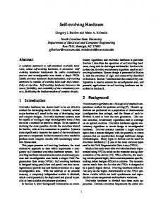
LUTs in Virtex II families can be easily configured as 4-input multiplexers by constraining the possible configurations to: 0000 0000 1111 1111 → sel = A1 0000 1111 0000 1111 → sel = A2 0011 0011 0011 0011 → sel = A3 0101 0101 0101 0101 → sel = A4 Implementing larger multiplexers requires the use of extra LUTs for multiplexing the new inputs. This is a useful general solution; however, sometimes it can be inefficient. For instance a 5-inputs multiplexer would use the double of LUTs than its 4-inputs counterpart. In this case it would be more optimal to use the multiplexers present in the FPGA slices for multiplexing the fifth input. In Figure 1 it is depicted the way in which the output of a LUT is connected to the slice output in a Virtex-II slice. By using the same technique used in [7], we found that the multiplexers selection bus can be controlled from the first and the fourth frame of the corresponding CLB column.
Figure 1 LUT and multiplexer in a Virtex II slice In Virtex II FPGAs, a CLB is composed of 4 slices arranged in 2 columns by 2 rows. The multiplexers’ configuration of the first slices’ column is contained in the first CLB frame (in total, there are 22 CLB frames per CLB column), while for the second slices’ column they are contained in the fourth CLB frame. The frame composition is depicted in Tableau 1. The configuration for each multiplexer consists in two bits (the selection lines), each bit contained in a byte ( Tableau 1). For G-mux the configuration bits are the second weakest bits in the byte, while for F-mux they are the second strongest bits. The multiplexer in Figure 1 is an F-mux with 3 inputs. The selection table is: 00→F, 01→F5, 10→unknown, 11→FXOR. For G-mux the selection table is slightly different for two reasons: it has four inputs and the order in the configuration bits is
inverted. Thus, the selection table is: 00→G, 01→SOPEXT, 10→GX, 11→GXOR. Tableau 1 Composition of the first and fourth CLB’s frames Description Size (# of bytes) Top IOB 12 Top slice G-mux (slice X0Y15)* 2 -1 Top slice F-mux (slice X0Y15)* 2 2nd slice G-mux (slice X0Y14)* 2 -1 2nd slice F-mux (slice X0Y14)* 2 … … Bottom slice F-mux (slice X0Y0)* 2 Bottom IOB 12 (* For the first frame of the first CLB column in a XC2V40).
By modifying these configuration bits, one can control the multiplexers’ selection, enhancing, in this way, the implementation efficiency of reconfigurable 5-inputs multiplexers. The functionality of the other bits in the frame doesn’t have any interest for us and remain unmodified during the system’s operation.
3. Random Boolean Networks Artificial neural networks (ANNs) [8] are information processing systems able to compute a function in an efficient and parallel way. ANNs are composed of a number of simple components called neurons, nodes or cells. These nodes are typically uniform or semi-uniform and are well suited for being adapted to fit a desired function. Neuron models can have different levels of complexity, ranging from simple Boolean function (McCulloch & Pitts) to biologically plausible models (Hodgkin & Huxley). In all cases, connectionism is a very important issue.
3.1 Randomly connecting systems Simplified connectionism schemas have shown to perform well for several problems. Layered ANNs are widely used for classification and control tasks, while cellular automata dynamics have been largely studied exhibiting interesting emergent behaviors. However, biological systems don’t use this simplistic connectionism, being it a critical point when building systems targeting self-adaptation and emergence. Several approaches using arbitrary connectionism have shown to perform well for several applications. Jaeger and Haas [9] have shown the suitability of echo state networks –randomly connected recurrent ANNs– to predict chaotic time series, improving accuracy by
2400 over previous techniques. Maass et al. [10] present their liquid state machines –randomly connected integrate and fire neurons–, which are able to classify noise-corrupted spoken words. A more simplistic node is used in random boolean networks [11], which consist of a set of N nodes implementing a boolean function, each one with K inputs, randomly connected among them. Several classifications are considered whether the nodes’ state update is performed in a synchronous or asynchronous way, and in a deterministic or random order. Even if RBN use Boolean functions as their basic node, there are not hardware implementations of such systems. The absence of implementations is mainly due to the random connectionism exhibited by the network and the high cost of connection flexibility in terms of hardware resources.
3.2 Cellular Programming in CA Cellular Automata (CA) are discrete time dynamical systems, consisting on an array of identical computing cells [12]. A cell is defined by a set of discrete states, and a rule for determining the transitions between states. On the array, states are synchronously updated according to the rule, which is function of the current state from the cell itself and the states of the surrounding neighbours. Non-uniform CA differ from their uniform counterpart in the state transition rule diversity exhibited by the non-uniform ones. Uniform CA constitute a sub-set of non-uniform CA, making the non-uniform ones a more general and powerful platform and, in the same way, more difficult to design. Evolutionary techniques have been used for finding non-uniform CA state transfer [13, 14] rules. Several evolutionary algorithms have been used for non-uniform CA: mainly genetic algorithms [13] and cellular programming [14]. Cellular Programming is an algorithm that considers a genome per cell instead of a genome for the whole system as typical evolving algorithms. When running the algorithm, initial node rules are initialized at random. Then, initial states are equally randomly initialized; we let the CA run for M iterations, and we repeat it for a number of different initial states. The fitness is assigned locally to each node. After computing the fitness, the genetic operators (reproduction, crossover, and mutation) are applied to genomes. In this algorithm these evolutionary operators act on a local manner, by limiting the reproduction and crossover operators to use genomes from neighbour cells. The algorithm is driven by nfi –
the number of fitter neighbours of cell i– in the following manner: - if nfi =0 (i is fitter than its neighbours) then rule i is unchanged - if nfi =1 (i has a fitter neighbour) then i is replaced by the fittest one, followed by mutation - if nfi ≥ 2 (i has two or more fitter neighbours) then i is replaced by a crossover of the two fittest ones, followed by mutation (A more detailed description of the cellular programming algorithm may be found in [14]).
3.3 Main differences between RBN and CA RBN differ in several fundamental aspects from non-uniform CA making difficult to apply the same rule-adaptation algorithms to both. a) RBN neighbourhood is asymmetric: if A state is an input to B, it does not implies that B state is an input to A; while in CA it does. b) RBN neighbourhood is non-uniform: if Ak is connected to Ak+1,it doesn’t imply that Ak+1 is connected with Ak+2; while for CA it does (for k+2 ≤ N). c) CA rules typically consider the topological order in the rule-inputs order: In a 3-inputs rule the input in the middle constitutes the cell state. While in RBN, inputs can have any order. These fundamental differences don’t allow to directly applying algorithms designed for CA to RBN. That’s the reason why, new algorithms or variations to old ones must be proposed.
3.4 Cellular Programming in RBN When implementing an algorithm like cellular programming to a given cellular structure for a given task, one must first analyze whether a genome that was good for a certain cell, can potentially be good for its neighbors. Let’s suppose, as an extreme case, two completely different nodes: an integrate and fire neuron and a fuzzy rule. The same genome having two possible different mappings to two different structures would certainly not perform well in both cases. Considering mainly the item c) of the previous subsection, one can deduce that a node’s genome that was useful for solving the firefly problem (details on the problem in section 6) having its current state as input, cannot be useful for a node that doesn’t have it. Because of that we have focus our study in a particular type of neighborhood and cell. Our cell consists in a Boolean function with 3 inputs: a random input, its own cell state, and a random input, in that order. This distribution of cell’s inputs allows us to use
the same structure and rule notation that is used in CA [12], while keeping a flexible neighborhood. Given, also, the neighborhood asymmetry described in the previous section one cannot directly use the standard Cellular Programming algorithm for adapting RBN rules. The concept of neighborhood does not have a placement or index connotation any more, but a connectivity one. This neighborhood paradigm generates new issues. The state of a given cell can be the input of many other cells or it can be completely source-less. On the other hand, one can be sure that there are two cells driving the inputs. This fact makes us consider as neighborhood the inputs to the cell instead of the outputs. Taking into account these considerations, one can apply the Cellular Programming algorithm, described in section 3.2, to RBN.
4. The hardware RBN cell array A hardware architecture of a cellular system allowing a completely arbitrary connectionism, constitutes a very hard routing problem. The main problem to face is the scalability. Allowing full connectionism in a 2x2 cellular system is an easy task. However, increasing size implies not only to increase the number of cells but also the size of the multiplexers selecting the nodes inputs. This fact makes the resource requirements to increase exponentially when increasing the amount of nodes. In this section, we propose an RBN cell array that allows full implementation scalability. It allows connecting any node with any other; however, some constraints must be introduced to the connectionism: the first connections to route don’t have congestion problems, but the further connections are constrained by the routing of the previously connected nodes. We outline two main advantages of our proposed architecture: implementation resource efficiency and direct genome mapping. Figure 2 illustrates the RBN cell array: it consists of an array of identical elements, each one containing a rule implemented in a look-up-table (LUT), a flip-flop storing the cells state, and flexible routing resources implemented in the form of multiplexers. In the 2-D case, each cell has 4 inputs and 4 outputs corresponding to its four cardinal points: north, west, south, and east, fitting well with the nowadays 2-D IC fabrication technology. Additional dimensions would require two more inputs per dimension. An output from the cell can be driven by the cell’s state or by any other input, allowing the outputs to act as a bypass from distant cell states. In a typical 2-D CA, outputs would be always driven by the cell’s state.
Cells’ state is updated by a rule –a Boolean function–. As cell outputs, rule inputs can be driven by any input or by the cell’s state. If two multiplexers select the same driver the 4-inputs rule becomes a 3inputs rule, existing also the possibility to become a 1input rule if all multiplexers select the same input.
Figure 2. RBN cell: rule and connectionism implementation Figure 3 shows an example of an implemented network. One can observe that while cell 3,1 has 4 inputs (N, S, E, and C), cell 3,3 has just 2 (N and E), and cell 1,3 has only 1 input (C) and is completely isolated from the other nodes. It must be also noticed the existence of drive-less nets in the array. The net created from cell 1,2, to 2,2, to 2,3, and to 1,3, has not driver, and has cell 2,3 as source. This drive-less net can be considered as a source of noise, maybe desirable for exploring fault-tolerant or noise-tolerant systems. However, in general it would be a nondesirable connection in the network.
One can envisage 3 ways of generating a random connectionism in this array. The first approach consists in randomly generating the sources for each node by randomly assigning a cell for driving each cell’s input. This approach corresponds to what is traditionally done in software implementations of RBN. This technique requires a further routing procedure in order to select the multiplexer’s states allowing the connections. For slightly large networks there is a very high probability for the design of being un-routable given congestion in the network. A possible solution can be to provide more RBN cells than required. In this way nodes can be distributed along the array and congestion problems may be reduced. For a deep analysis of congestion probability in 4-neighbors cells see [15]. The second approach consists in randomly assigning values to multiplexers’ selections. This solution avoids congestion problems without requiring the addition of useless cells, by restricting the amount of possible network configurations to the ones allowed by the network (in the previous approach it was not the case). Its main advantage is that no routing phase is needed, while the remaining problem is that it can easily generate drive-less nets. The third approach, and the one implemented by us, consists in randomly generating values of multiplexers’ selections, while forcing random drivers for drive-less nets. The following pseudo-code depicts an algorithm allowing to randomly creating drive-less free networks: • Initially, every connection is drive-less. • While drive-less connections exist do: o Begin a net construction by randomly selecting a drive-less connection (current connection) o While current net is drive-less do: Assign a random value to the current connection multiplexers’ selection If selection is C or a connection already used for another net, the current net has found a driver Elseif selection is a connection of the current net (it will form a drive-less loop) force selection to C. Otherwise, update current connection with the connection driving the current net o end while • end while
This algorithm guarantees that every connection will be part of a net, and every net will be driven by a cell. Anyway, the algorithm doesn’t prevent the formation of isolated nodes or subnets.
5. Setup of the self-reconfigurable system Figure 3 Example of a RBN cell array configuration
In this section we present the FPGA platform that self-reconfigures the RBN connectionism and Boolean
rules through the ICAP. Our platform consists in a Microblaze soft-processor running on a Virtex-II FPGA from Xilinx. The main advantage of using the vendor-provided soft-processor is the high number of IP peripherals available, and the user-friendly programming environment provided.
further synthesized, placed, and routed, by automatic tools. Implementing the RBN cell in this way requires 18 Virtex II slices –i.e. 5 CLBs–, while implementing it by defining a hard-macro for further reconfiguring the logic supporting it, just requires 4 slices –i.e. 1 CLB– as depicted in Figure 5.
5.1. General System Description The complete system schematic is depicted in Figure 4. A Microblaze soft-processor from Xilinx runs an adaptive algorithm. The program is stored in an internal BRAM, and an external SRAM is used for data storing – i.e. genome storing in the case of evolving algorithms. The system interfaces through an UART peripheral with the external world, providing a console for monitoring and debugging from a PC. The RBN cell array to be adapted can be accessed for reading or for writing states through general purpose I/O interfaces; anyway, connections and rule modifications are exclusively performed through the HWICAP peripheral. The HWICAP module allows the Microblaze to read and write the FPGA configuration memory through the Internal Configuration Access Port (ICAP) at run time, enabling our adapting algorithm to modify the circuit’s structure and functionality during the circuit’s operation, specifically, in our case: RBN connections and rules.
Figure 4. Self-reconfigurable platform setup
5.2 RBN cell array implementation The RBN cell is implemented as a hard macro. Figure 5 depicts how it is implemented by using the four slices in a CLB. The RBN cell has 4 inputs from its neighbors: N_in, W_in, S_in, and E_in (summarized as NWSE_in). It has, in the same way, 4 outputs to its neighbors: N_out, W_out, S_out and E_out. Three global input signals are included for system control: CLK, EN, and RST. And an output signal for observing the cell’s state from the processor. A common technique, alternative to using the FPGA’s low level resources, is to define the RBN cell as a virtual reconfigurable circuit. In this case, the reconfigurable circuit is described by a HDL and
Figure 5 Hard-macro for the RBN cell
6. Example task: Firefly In some areas of south-east Asia, one can find certain species of bioluminescent insects called fireflies. These insects emit flashes of light as mating communication signals. When forming a group fireflies flash rhythmically in a synchronized way. This emergent behavior exhibited by fireflies constitutes a biological spectacle, amazing from the esthetical and scientific point of view. In artificial cellular systems, the firefly synchronization problem consists in synchronizing the firing of a set of 2-state nodes. Nodes are initialized at a random state, and after a number of iterations each node must swap from one state to the other, synchronizing with his neighbors. We have used this problem for validating our RBN cell. In our implementation we use a 5x6 RBN cell array, implemented on an array of 5x6 CLBs. The microblaze processor initializes the Cell Array by randomly configuring the RBN connectionism. Then the processor executes the Cellular Programming algorithm for RBN described in section 3. Through the HWICAP peripheral we map the genome contents on the frames containing the LUT and multiplexer contents. In this way, the system rewrites 4 frames per array column when reconfiguring connectionism (24 frames in our example) and 1 frame per column when updating rules (6 frames for us). Once frames are re-configured, one can test the RBN through the reading and writing interfaces. The fitness is computed by the Microblaze soft-processor, by reading the nodes’ state. For computing the fitness, we read the states when completed the number of iterations, we compute the phase of the majority of the nodes, and then we let the RBN execute four more
iterations. If the sequence is 0-1-0-1 (or 1-0-1-0) when the majority phase is 1 (or 0) the fitness is 1, otherwise the fitness is 0. On that way we accumulate the fitness for 20 initial states for obtaining the final fitness. Afterward, a new genome for each cell is generated as described in section 3. For measuring the performance of our algorithm, we ran 1000 simulations. Each simulation consists in: • Random initialization of connections and rules. • For 100 generations do: o For 20 different initial states do: Random initialization of cell states Let the RBN run for 34 iterations. Compute partial fitness for each cell o For each cell, compute total fitness as the sum of partial fitness. o Update cell rule according to the cell fitness. • Deliver the best result – the one with the highest average fitness. Our platform achieves to successfully finding RBN able to synchronize the switching of the states. Among the 1000 simulations, 3.4% managed to fully synchronize. It must be noticed that the result is highly dependant of the initial connections: connectivity and initial rules. A random network with isolated nodes will never fully synchronize, as well as a network not containing initial “good” rules will have difficulties in converging to a good solution.
7. Conclusions In this paper, we presented an approach for efficiently implementing flexible connecting systems with commercial FPGAs. The low level utilization of FPGA basic components guarantees the optimality of the approach. RBN have been used as case study given their needs of connectionism flexibility and their node’s analogy to hardware. A second important aspect of this paper is the proposal of an on-chip and on-line self-adaptive system on a reconfigurable platform, which has been always an important issue in self-adapting systems. This paper describes how to implement it, in an efficient way, on nowadays commercial devices. The proposed system constitutes a novel system approach for evolving hardware. Our platform has shown to be suitable for coevolving RBN rules, and the same approach can be easily extended to other connectionism systems – like evolving artificial neural networks or liquid state machines – just by plugging them to a hard macro allowing the flexible connectionism. The system on chip supporting these reconfiguration capabilities provides the hardware platform to support the so called on-chip and on-line
self-reconfigurable adaptable systems, by providing the flexibility needed by a real phenotype modification on the evolved hard individual. RBN constitute an interesting test-bench given their universality, and their straight-forward analogy with digital circuits.
8. References [1] M. Sipper, E. Sanchez, D. Mange, M. Tomassini, A. Perez-Uribe, and A. Stauffer, "A Phylogenetic, Ontogenetic, and Epigenetic View of Bio-Inspired Hardware Systems", IEEE Transactions on Evolutionary Computation, vol. 1, pp. 83-97, 1997. [2] S. Trimberger, Field-programmable gate array technology. Boston: Kluwer Academic Publishers, 1994. [3] Xilinx_Corp., "Virtex-II Platform FPGA User Guide": www.xilinx.com, March 2005. [4] Xilinx_Corp., "XAPP 290: Two Flows for Partial Reconfiguration: Module Based or Difference Based": www.xilinx.com, Sept, 2004. [5] G. Mermoud, A. Upegui, C. A. Peña-Reyes, and E. Sanchez, "A Dynamically-Reconfigurable FPGA Platform for Evolving Fuzzy Systems", in The 8th International Work-Conference on Artificial Neural Networks (IWANN'2005), 2005. [6] B. Blodget, P. James-Roxby, E. Keller, S. McMillan, and P. Sundararajan, "A self-reconfiguring platform", Proceedings of Field-Programmable Logic and Applications, LNCS, vol. 2778, pp. 565-574, 2003. [7] A. Upegui and E. Sanchez, "Evolving hardware by dynamically reconfiguring Xilinx FPGAs", Evolvable Systems: From Biology to Hardware, LNCS, vol. 3637, pp. 56-65, 2005. [8] S. S. Haykin, Neural networks : a comprehensive foundation, 2nd ed. Upper Saddle River, N.J.: Prentice Hall, 1999. [9] H. Jaeger and H. Haas, "Harnessing nonlinearity: Predicting chaotic systems and saving energy in wireless communication", Science, vol. 304, pp. 78-80, 2004. [10] W. Maass, T. Natschlager, and H. Markram, "Real-time computing without stable states: A new framework for neural computation based on perturbations", Neural Computation, vol. 14, pp. 2531-2560, 2002. [11] C. Gershenson, "Classification of random boolean networks", Proceedings of the Eight International Conference on Artificial Life., pp. 1–8, 2002. [12] S. Wolfram, A new kind of science. Champaign, IL: Wolfram Media, 2002. [13] M. Mitchell, J. P. Crutchfield, and P. T. Hraber, "Evolving Cellular-Automata to Perform Computations - Mechanisms and Impediments", Physica D, vol. 75, pp. 361-391, 1994. [14] M. Sipper, "Co-evolving non-uniform cellular automata to perform computations", Physica D-Nonlinear Phenomena, vol. 92, pp. 193-208, 1996. [15] Y. Thoma, "Tissu Numérique Cellulaire à Routage et Configuration Dynamiques". PhD Thesis. Lausanne, Switzerland: EPFL, 2005.