IEEE SIGNAL PROCESSING LETTERS, VOL. 20, NO. 7, JULY 2013
701
Exact Fast Computation of Optimal Filter in Gaussian Switching Linear Systems Stéphane Derrode and Wojciech Pieczynski
Abstract—We consider triplet Markov Gaussian linear systems , where is hidden continuous random sequence, is hidden discrete Markov chain, is observed continuous is Gaussian conditionally on . In random sequence, and the classical “Conditionally Gaussian Linear State-Space Model” (CGLSSM), optimal filter is not workable with a reasonable complexity. The aim of the paper is to propose a new model, quite close to the CGLSSM, belonging to the general and recently proposed family of models, called “Conditionally Markov Switching Hidden Linear Models” (CMSHLMs), in which the computation of optimal filter with complexity linear in the number of observations is feasible. The new model and related filtering are immediately applicable in all situations where the classical CGLSSM is used via approximated filtering. Index Terms—Conditionally Gaussian linear state-space model, Kalman filter, optimal statistical filter, switching systems.
I. INTRODUCTION
L
ET
us
consider
three
random
sequences and , where the sequences and take their values in and respectively, while is discrete finite, each taking its values in . Both and are hidden, while is observed. The process can be seen as modeling the random “switches” of the distributions linked with , which can be of utmost importance in non stationary situations. The “optimal filter” problem we deal with in this paper consists in the sequential search of from . More precisely, with usual notations for conditional probabilities and conditional expectations and variances, we search and from and . The optimal filter is then given by and its variance by with . Such a problem is of importance in numerous situations and hundreds of papers deal with different solutions for several decades. In this paper we deal with the simple “Conditionally Gaussian Linear Manuscript received March 07, 2013; accepted April 10, 2013. Date of publication May 03, 2013; date of current version May 28, 2013. The associate editor coordinating the review of this manuscript and approving it for publication was Prof. Peng Qiu. S. Derrode is with Centrale Marseille Aix Marseille Universit, CNRS, Institut Fresnel, UMR 7249, 13013 Marseille, France (e-mail:
[email protected]). W. Pieczynski is with Telecom SudParis, CITI Dpt, CNRS UMR 5157, Evry, France (e-mail:
[email protected]). Digital Object Identifier 10.1109/LSP.2013.2261494
State-Space Models” (CGLSSMs) [1], [2], though the presented results are likely to be extended to other more sophisticated models in references mentioned above [3]–[5]. There exists numerous applications, among which tracking problems are of importance [6]. In CGLSSMs the distribution of is obtained by setting together two classical and widely used models that are “Hidden Markov Chains” (HMCs) and “Linear Gaussian State-Space Models” (LGSSMs). Roughly speaking, has the structure of an HMC and, conditionally on is a LGSSM. Then, when is known, the problem is solved by the classical Kalman filter and, when is not known, the problem has no known solution with a reasonable complexity and approximate methods are used. The aim of the paper is to introduce an alternative model, which is not more complicated than CGLSSM, which is close to it, and which does allow fast and exact optimal filtering. More precisely, a CGLSSM is given of and the recurby the distribution sions verifying (1) (2) (3) with appropriate matrices depending on switches, and white Gaussian noises independent each from the other and is such that for each independent from . In such a model the marginal distributions are, in the general case, mixtures of Gaussian distributions with a number of components exponentially increasing with . We propose two contributions: 1) we modify the CGLSSM above by replacing with in such a way that in the modified model, the marginal distributions give the Gaussian. Thus conditional distributions the general form of margins does not depend on —however the parameters can vary with —, which seems to us to better suit real situations; 2) we associate with the modified model, called “Model 1”, a new model, called “Model 2”, which belongs to the “Conditionally Markov Switching Hidden Linear Models” (CMSHLMs) family introduced in [7]—and thus in which fast exact filtering is possible—and which is “close” to the Model 1. In particular, for each and are identical in both models. Then we specify how the fast optimal filter runs.
1070-9908/$31.00 © 2013 IEEE
702
IEEE SIGNAL PROCESSING LETTERS, VOL. 20, NO. 7, JULY 2013
Let us insist on the fact that we do not consider Model 2 as an approximation of a given Model 1, but rather as an alternative model, close to Model 1, but allowing fast optimal filtering. II. MODIFIED CGLSSM AND ASSOCIATED CMSHLM and , Let us denote and let us consider the CGLSSM defined by (1)–(3) above. Conditionally on , the covariance matrix of the Gaussian distribution of depends on . Indeed, we have classically the recursion and thus the marginal distributions are mixtures of Gaussian distributions. Let us search for a model having desired marginal Gaussian distributions , and thus such that its covariance matrix only depends on . Such models can be defined re, cursively: for a given desired sequence let us consider the following CGLSSM, called Model 1: verifies (1) and (4) (5) (6) We can also say that Model 1 is a classic CGLSSM in which depends on both and in such a way that . Reporting given by (4) into (6), (4)–(6) can be written (7) with
and
defined by (8)
(9) We define the Model 2 associated with the Model 1 given by (1), (7)–(9) as the model verifying (10) with
given by (11)
with
Thus
is recursively given from and , the covariance matrices common to Model 1 and Model 2. Finally, for each , the marginal Gaussian distributions are the same in Model 1 and Model 2. To see the difference between them, let us compute the equation shown at the bottom of the page. We have for Model 1 and Model 2 respectively
We find that
, but whereas
. Thus we can state the following result, which specifies the “closeness” of both models. Proposition 1: Let us consider the Model 1 given by eq. (1), (7)–(9), and the associated Model 2 given by eq. (1), (10)–(13). We can state: 1) For each , the Gaussian conditional distributions , and are the same in models 1 and 2, and the only difference comes from . In particular, and , which are used in building Model 1, are the same; 2) Distribution is Markov in both models with identical distribution, while is Markov in Model 2, but not in Model 1. Proof: Point 1) comes from the very construction of the Model 2 above. To show that is Markov with identical distributions in Model 1 and Model 2, we remark that eq. (4) is valid for both of them. The fact that is not Markov in Model 1 is a classic property. To show that it is Markov in Model 2, let us first remark that the second line in matrix is of the form and let us set the second line of the matrix . We have, according to (10), where is independent from . This implies that is Markov. Let us show that Model 2 is a “Conditionally Markov Switching Hidden Linear Model” (CMSHLM) introduced in [7]. The latter verifies:
(12) and
such that the covariance is the same as in Model 1, which gives
matrix (14) (13)
(15)
DERRODE AND PIECZYNSKI: EXACT FAST COMPUTATION OF OPTIMAL FILTER
with appropriate and
from
matrices,
and as follows:
appropriate white noise, appropriate vectors. and can then be computed from with complexity independent
703
and variance ( is given in eq. (12)). Using the classical Gaussian conditioning rule we can say that the distribution is then Gaussian with mean and variance respectively given by and . Then we can state, according to classic properties of Gaussian laws, that (15) is verified with
(16) (20) (17)
(18)
(19) Proposition 2: Model 2 defined with (1) and (10)–(13) is a CMSHLM (14)–(15). Proof: Let
Let us we can
first verify write
(14).
is .
cording
to
(1) we have and, according
Markov
and Ac-
Finally, the optimal filter in the switching system (4)–(6) is: for given , and 1) consider and verifying (5), with (6) and with (11), which provide (12); 2) compute with (13); 3) compute and with (20); 4) compute , knowing that is Gaussian with mean and covariance matrix ; 5) compute and with (16)–(20). III. EXPERIMENTS Let us consider (both and are real valued processes), and the stationary case where the distributions of are independent from in both models. and . Thus Each takes its values in and we set, for both models, and for : and . Then for we have for Model 1
to
(10)–(11), we have . The two equali. ties give Let us then verify (15). According to (10) the distribution is Gaussian with mean According to eq. (11) and (13) the associated Model 2 is given by the equation shown at the bottom of the page,
704
IEEE SIGNAL PROCESSING LETTERS, VOL. 20, NO. 7, JULY 2013
TABLE I MSE ERROR OF F1, F2 AND F3 FILTERS WITH
The presented results, and different other results not reported here, show that it is difficult to obtain a significant difference between F1 and F2, which is our main conclusion. IV. CONCLUSION
TABLE II MSE ERROR OF F1, F2 AND F3 FILTERS WITH
We proposed a new model, very close to the classic “Conditionally Gaussian Linear State-Space Model” (CGLSSM), but allowing, in spite of switches, a fast optimal statistical filter. This property is due to the fact that the model proposed belongs to the family of models recently introduced in [7]. The distribution of the switching sequence, that of the hidden continuous sequence, and that of each observation at time , conditional on the switch and the state at , are strictly the same in both models. So the new model can be immediately used in all situations the classical CGLSSM is. Simulation experiments numerically show that the new model is fairly identical to CGLSSM. The main conclusion is that the two models are so close that it is difficult to see any difference at results level, at least in the case of real-valued sequences considered. In addition, the results obtained with the new model with known switches are very close to those obtained when the switches are unknown. As perspective for further works let us mention that we consider the filtering problem in this paper, but the recent models can also be used to deal with prediction [10] and smoothing [11]. Another perspective would be the parameter estimation problem [12], [13]. REFERENCES
which
gives
and by (20). Finally, the two models are and by the defined by the parameters distribution . We present two series of experiments. In the first series, data are sampled according to Model 1, and in the second one, data are sampled according to Model 2. Both series were filtered according to three methods: (F1) is the Model 1 based optimal filter with known switches, (F2) is the Model 2 based optimal filter with known switches (conditionally on , Model 2 also is a classical system but more general situations, where it would be a Pairwise Markov Model, in which the classical Kalman filter is workable [8], [9], could be considered), and (F3) is the Model 2 based optimal filter with unknown switches. The sample size is and we consider and . We consider two cases: (Table I) and (Table II). Then we consider two possible values 0.98 and 0.80 for and two possible values 0.5 and 1.0 for . For filter F3, we also report the error rate while estimating the switches by maximizing (notice that these estimates of switches are not used in F3). The results, which are means of 300 independent experiments are expressed in term of the Mean Square Error (MSE).
[1] C. Andrieu, M. Davy, and A. Doucet, “Efficient particle filtering for jump Markov systems. Application to time-varying autoregressions,” IEEE Trans. Signal Process., vol. 51, no. 7, pp. 1762–1770, Jul. 2003. [2] O. Cappé, E. Moulines, and T. Ryden, Inference in Hidden Markov Models. Berlin, Germany: Springer-Verlag, 2005. [3] O. L. V. Costa, M. D. Fragoso, and R. P. Marques, Discrete Time Markov Jump Linear Systems. Berlin, Germany: Springer-Verlag, 2005. [4] C.-J. Kim and C. R. Nelson, State-space Models with Regime Switching. Cambridge, MA, USA: MIT Press, 1999. [5] B. Ristic, S. Arulampalam, and N. Gordon, Beyond the Kalman Filter: Particle Filters for Tracking Applications. Norwell, MA, USA: Artech House, 2004. [6] M. Arulampalam, S. Maskell, N. Gordon, and T. Clapp, “A tutorial on particle filters for online nonlinear/non-Gaussian Bayesian tracking,” IEEE Trans. Signal Process., vol. 50, no. 2, pp. 174–188, Feb. 2002. [7] W. Pieczynski, “Exact filtering in conditionally Markov switching hidden linear models,” Compt. Rend. Math., vol. 349, no. 9–10, pp. 587–590, May 2011. [8] W. Pieczynski and F. Desbouvries, “Kalman filtering using pairwise Gaussian models,” in Proc. IEEE Int. Conf. Acoustics, Speech and Signal Processing (ICASSP’03), Hong Kong, Apr. 2003. [9] V. Nemesin and S. Derrode, “Robust blind pairwise Kalman algorithms using qr decompositions,” IEEE Trans. Signal Process., vol. 61, no. 1, pp. 5–9, Jan. 2013. [10] N. Bardel and F. Desbouvries, “Exact Bayesian prediction in a class of Markov-switching models,” Meth. Comput. Appl. Probabil., vol. 14, no. 1, pp. 125–134, Mar. 2012. [11] W. Pieczynski, “Exact smoothing in hidden conditionally Markov switching linear models,” Commun. Statist.—Theory Meth., vol. 40, no. 16, pp. 2823–2829, Aug. 2011. [12] E. Fox, E. B. Sudderth, M. I. Jordan, and A. S. Willsky, “Bayesian nonparametric methods for learning Markov switching processes,” IEEE Signal Process. Mag., vol. 27, no. 6, pp. 43–54, 2010. [13] M. I. Jordan, Learning in Graphical Models. Cambridge, MA, USA: MIT Press, 1998.