Subbalaxmi Rao, and my sister Mrs. Deepti Rao Vishwakarma for their unwavering supporting and .... 3.4.1 Non-Extrapolating Sigma Method . .... 5.1.8 Brezinski's Theta Algorithm . ...... where δni is the Kronecker delta, defined by (3.35). â©. â¨. â§. = = ...... It was observed, for these test systems, that the HEPF bus-types at the ...
Exploration of a Scalable Holomorphic Embedding Method Formulation for Power System Analysis Applications by Shruti Dwarkanath Rao
A Dissertation Presented in Partial Fulfillment of the Requirements for the Degree Doctor of Philosophy
Approved July 2017 by the Graduate Supervisory Committee: Daniel Tylavsky, Chair Anamitra Pal John Undrill Vijay Vittal
ARIZONA STATE UNIVERSITY August 2017
ABSTRACT The holomorphic embedding method (HEM) applied to the power-flow problem (HEPF) has been used in the past to obtain the voltages and flows for power systems. The incentives for using this method over the traditional Newton-Raphson based numerical methods lie in the claim that the method is theoretically guaranteed to converge to the operable solution, if one exists. In this report, HEPF will be used for two power system analysis purposes: a. Estimating the saddle-node bifurcation point (SNBP) of a system b. Developing reduced-order network equivalents for distribution systems. Typically, the continuation power flow (CPF) is used to estimate the SNBP of a system, which involves solving multiple power-flow problems. One of the advantages of HEPF is that the solution is obtained as an analytical expression of the embedding parameter, and using this property, three of the proposed HEPF-based methods can estimate the SNBP of a given power system without solving multiple power-flow problems (if generator VAr limits are ignored). If VAr limits are considered, the mathematical representation of the power-flow problem changes and thus an iterative process would have to be performed in order to estimate the SNBP of the system. This would typically still require fewer power-flow problems to be solved than CPF in order to estimate the SNBP.
i
Another proposed application is to develop reduced order network equivalents for radial distribution networks that retain the nonlinearities of the eliminated portion of the network and hence remain more accurate than traditional Ward-type reductions (which linearize about the given operating point) when the operating condition changes. Different ways of accelerating the convergence of the power series obtained as a part of HEPF, are explored and it is shown that the eta method is the most efficient of all methods tested. The local-measurement-based methods of estimating the SNBP are studied. Nonlinear Thévenin-like networks as well as multi-bus networks are built using model data to estimate the SNBP and it is shown that the structure of these networks can be made arbitrary by appropriately modifying the nonlinear current injections, which can simplify the process of building such networks from measurements.
ii
ACKNOWLEDGMENTS First and foremost, I would like to express my deepest gratitude to my advisor, Dr. Daniel J. Tylavsky, for giving me the opportunity to work with him on some very interesting research projects. I sincerely thank him for his invaluable guidance and constant encouragement. His critical insights and never-fading enthusiasm about the subject have been most critical in the completion of this work. I would like to thank my committee members, Dr. Anamitra Pal, Dr. John Undrill and Dr. Vijay Vittal for taking the time to give their invaluable feedback. I would also like to thank all the other faculty members I studied with, for the various learning and growth opportunities over the past five years. I would like to thank Yang Feng and Muthu Kumar Subramanian for the guidance provided when I started working on this project and the numerous insights they gave about the algorithm. I would also like to thank Yuting Li, Yujia Zhu, Qirui Li and Chinmay Vaidya who have been great team members to work with. In addition, I would like to express my appreciation to Salt River Project, for providing financial support.
Finally, I would like to thank my family and friends, for their unfaltering love and support. I would especially like to thank my parents Mr. Dwarkanath Rao and Mrs. Subbalaxmi Rao, and my sister Mrs. Deepti Rao Vishwakarma for their unwavering supporting and encouragement, despite being far away. iii
TABLE OF CONTENTS Page
LIST OF FIGURES ...................................................................................................... xi LIST OF TABLES ................................................................................................... xviii NOMENCLATURE .................................................................................................... xx CHAPTER 1
INTRODUCTION ........................................................................................... 1 1.1
The Power-Flow Problem And Its Solution Using The Holomorphic Embedding Method ................................................................................. 1
2
1.2
Objectives ................................................................................................ 4
1.3
Organization ............................................................................................. 7
LITERATURE REVIEW .............................................................................. 10 2.1 2.1.1
Continuation Power Flow ................................................................... 12
2.1.2
Other Methods For SNBP Estimation ................................................ 18
2.2
3
Saddle Node Bifurcation Point Estimation ............................................ 10
Network Reduction Methods ................................................................. 21
2.2.1
Ward Reduction .................................................................................. 22
2.2.2
Other Methods Of Network Reduction .............................................. 23
HEPF-BASED METHODS OF ESTIMATING THE SADDLE-NODE BIFURCATION POINT OF A SYSTEM .................................................... 26 iv
CHAPTER 3.1
Page Formulation To Scale All Loads And Generations Uniformly .............. 27
3.1.1
Calculating The Germ Using HEPF ................................................... 33
3.1.2
Recurrence Relations For The Scalable Form .................................... 36
3.2
Non-Scalable Formulation ..................................................................... 40
3.3
Using The Roots Of Padé Approximants To Estimate The SNBP .......... 42
3.4
The Sigma Methods ............................................................................... 44
3.4.1
Non-Extrapolating Sigma Method ..................................................... 46
3.4.2
Extrapolating Sigma Method.............................................................. 48
3.4.3
Traditional Modal Analysis To Determine The Weak Buses In A System ................................................................................................ 61
3.5
Numerical Results For Scaling All Loads Uniformly............................ 64
3.6
Incorporating Var Limits In The SNBP Estimation .............................. 73
3.7
Direction-Of-Change Scaling Formulation............................................ 76
3.7.1
Using The Direction-Of-Change Scaling Formulation To Determine The Weak Buses In The System ......................................................... 78
3.8
Numerical Results For Direction-Of-Change Scaling Formulation ...... 82
3.9
Proposed ZIP-Load Model For HEPF ................................................... 84
3.10
Conclusions ............................................................................................ 86
v
CHAPTER 4
Page
NETWORK EQUIVALENCING FOR DISTRIBUTION SYSTEMS USING HEPF................................................................................................ 88 4.1
Three HEPF-Based Network Reduction Methods ................................. 89
4.1.1
Obtaining The Series Branch As A Function Of α............................. 89
4.1.2
Obtaining The Shunt Admittance As A Function Of α ...................... 91
4.1.3
Obtaining The Complex Power Injection As A Function Of α .......... 92
4.2
Numerical Results For Uniform Load Scaling ...................................... 94
4.3
Different Methods Of Estimating Alpha For Non-Uniform Load Changes ............................................................................................... 100
A.
Projection Of The Vector Of New Loads On The α Line ................ 101
B.
Ratio Of The Sum Of Apparent Powers Of All External Buses ...... 101
C.
Mean Of Projection Of Each External New Load On Its α Line ..... 101
D.
Ratio Of Net Apparent Power In The External System ................... 102
E.
Mean Of Ratios Of Apparent Powers For All External Buses ......... 102
4.4
Numerical Results For Non-Uniform Load Changes .......................... 102
4.5
Network
Reduction
Using
Direction-Of-Change
Scaling
Formulation ......................................................................................... 108
vi
CHAPTER 4.5.1
Page Obtaining The Incremental Complex Power Injection As A Function Of α ................................................................................................... 109
4.6 5
Conclusions .......................................................................................... 112
THEORETICAL CONVERGENCE GUARANTEE VERSUS NUMERICAL CONVERGENCE BEHAVIOR OF THE HOLOMORPHICALLY EMBEDDED POWER FLOW METHOD ........ 114 5.1
Different Methods Of Accelerating The Convergence Of HEPF Series ................................................................................................... 115
5.1.1
Matrix Method .................................................................................. 116
5.1.2
Aitken’s Δ2 Method .......................................................................... 120
5.1.3
Wynn’s Epsilon Method ................................................................... 122
5.1.4
Eta Method ....................................................................................... 125
5.1.5
Viskovatov
Method
(Continued
Fraction
And
Three-Term
Recursion) ........................................................................................ 127 5.1.6
Van Wijngaarden Transformation .................................................... 129
5.1.7
Wynn’s Rho Algorithm .................................................................... 130
5.1.8
Brezinski’s Theta Algorithm ............................................................ 131
vii
CHAPTER 5.2
Page Comparison Of The Different Methods Of Analytic Continuation For The Power-Flow Problem ........................................................................... 133
5.3
Hermite-Padé Approximants ............................................................... 141
5.3.1
Algebraic Hermite-Padé Approximants ........................................... 142
5.3.2
Integral Hermite-Padé Approximants .............................................. 143
5.4
Relation Of Algebraic Hermite-Padé Approximants To The HEPF Solution ............................................................................................... 144
6
5.5
Numerical Results For Quadratic Approximants................................. 147
5.6
Conclusions .......................................................................................... 151
LOCAL-MEASUREMENT-BASED METHODS OF STEADY-STATE VOLTAGE STABILITY ANLAYSIS ....................................................... 154 6.1
Local-Measurement-Based Methods Of Estimating The Steady-State Voltage Stability Margin ..................................................................... 154
6.2
Effect Of Discrete Changes On Local Measurement-Based Methods Of Estimating The Steady-State Voltage Stability Margin ...................... 164
6.2.1
Effect Of Generator Var Limits........................................................ 165
6.2.2
Effect Of Other Discrete Changes .................................................... 171
6.2.3
Limit-Induced Bifurcation Points ..................................................... 174
6.3
Validation Of Pseudo-Measurements Obtained Using HEPF ............. 176 viii
CHAPTER 6.4
Page Developing A Thévenin-Like Network Using HE Reduction ............. 177
6.4.1
Steps Involved In Obtaining The Thévenin-Like Network .............. 178
6.4.2
Impact Of Modeling Loads As Nonlinear Currents Or Nonlinear Impedances ....................................................................................... 190
6.4.3
Arbitrary Thévenin-Like Networks .................................................. 193
6.4.4
Maximum Power-Transfer Condition In The Presence Of A Variable Voltage Source ................................................................................. 197
7
6.4.5
Some Implementation Details .......................................................... 206
6.4.6
Multi-Bus Reduced-Order Equivalent Networks ............................. 211
6.5
Revisiting The Sigma Method ............................................................. 215
6.6
Conclusions .......................................................................................... 220
CONCLUSION AND FUTURE WORK .................................................... 222 7.1
Summary .............................................................................................. 222
7.2
Future Work ......................................................................................... 225
REFERENCES
...................................................................................................... 226
APPENDIX A
DERIVATION OF EQUIVALENCY BETWEEN AITKEN’S Δ2 METHOD AND PADÉ APPROXIMANTS ................................................................ 239
ix
APPENDIX B
Page
COMPARISON OF AITKEN’S Δ2 AND WYNN’S Ε METHODS FOR THE LN(1+X) SERIES .............................................................................. 243
C
COMPARING PADÉ APPROXIMANTS, AITKEN’S Δ2, EPSILON AND ETA METHODS FOR GREGORY’S PI SERIES ..................................... 246
D
PROOF THAT THE HEPF SERIES OBTAINED IS THE MACLAURIN SERIES ...................................................................................................... 249
x
LIST OF FIGURES Figure
Page
2.1 Solutions Of A Two-Bus Dc System Vs. Load ............................................. 11 3.1 Two-Bus System Diagram ............................................................................. 44 3.2 Plot Of σi Vs. σr At α = 1.88 And α = 3.1 For The IEEE-118 Bus System ... 52 3.3 Plot Of σ Condition Vs. α For The IEEE-118 Bus System ............................ 53 3.4 Plot Of Vr(α) Vs. α For The IEEE-14 Bus System ........................................ 56 3.5 Plot Of Radicand Of (3.57) Vs. α For The IEEE-14 Bus System.................. 59 3.6 Plot Of Radicand Of (3.57) Vs. α For Buses With Smaller Poles/Zeros In The IEEE-14 Bus System.................................................................................... 59 3.7 SNBP Obtained Using Different Methods ..................................................... 68 3.8 Magnitude Of The Radicand Of (3.57) For Bus 9 Vs. Number Of Terms In The Series.................................................................................................. 69 3.9 Predicted SNBP Using Roots Of The Numerator Vs. Number Of Terms In The Series ............................................................................................................ 70 3.10 Poles/Zeros Of A Two-Bus System, Modeled To Be Beyond The SNBP .. 73 4.1 Two-Bus Equivalent With Series Branch As Function Of α ......................... 90 4.2 Two-Bus Equivalent With Shunt Admittance As A Function Of α .............. 91 4.3 Two-Bus Equivalent With Power Injection As Function Of α ...................... 93 4.4 Radial 14-Bus Network.................................................................................. 94 xi
Figure
Page
4.5 Magnitude Of Y(α), Along The Real α Line ................................................. 97 4.6 Error In Voltage Magnitude, Along The Real α Line .................................... 98 4.7 Percentage Error In Slack Bus Power, Along The Real α Line ..................... 99 4.8 Magnitude Of S3(α), Along The Real α Line ............................................... 100 4.9 Error In Voltage Magnitude, Using S(α) Reduction .................................... 104 4.10 Percent Error In Slack Bus Power, Using S(α) Reduction ........................ 104 4.11 Error In Voltage Magnitude, Using S(α) Reduction .................................. 105 4.12 Percent Error In Slack Bus Power, Using S(α) Reduction ........................ 106 4.13 Three-Bus Test System .............................................................................. 107 4.14 Voltage Magnitude Error For 3-Bus System, Ward Reduction ................. 107 4.15 Voltage Magnitude Error For 3-Bus System, S(α) Reduction ................... 107 4.16 Two-Bus Equivalent With Incremental Power Injection As Function Of α ................................................................................................................. 109 4.17 Error In Voltage Magnitude Along The ‘α Line’ For The Δs(α) Reduction Of The 14-Bus System .................................................................................... 111 4.18 Percent Error In Slack Bus Power Along The ‘α Line’ For The Δs(α) Reduction Of The 14-Bus System ............................................................. 111 5.1 Convergence Behavior Of Different Algorithms To The Power Series Of The 118-Bus System ......................................................................................... 134
xii
Figure
Page
5.2 Convergence Behavior Of Different Algorithms To The Power Series Of The 300-Bus System ......................................................................................... 135 5.3 Convergence Behavior Of Different Algorithms To The Power Series Of The 6057-Bus ERCOT System ......................................................................... 136 5.4 Convergence Behavior Of Different Algorithms To The Bus Voltage Power Series Of The 118-Bus System With The Loading Of The System Close To Its SNBP Loading. ..................................................................................... 137 5.5 Number Of Terms Needed For Convergence, ERCOT ............................... 138 5.6 Diagonal Vs. Near-Diagonal Padé-Approximant Using Matrix Method, ERCOT ...................................................................................................... 139 5.7 Two-Bus System Diagram ........................................................................... 144 5.8 Padé Approximation Vs. Quadratic Approximation For Two-Bus System 146 5.9 Performance Of Quadratic Approximation For The IEEE 14-Bus System . 148 5.10 Performance Of Quadratic Approximation For The IEEE 118-Bus System ........................................................................................................ 149 6.1 Thévenin Equivalent At The Bus Of Interest .............................................. 154 6.2 Thévenin Impedance And Load Impedance ................................................ 156 6.3 |Zth| And |Eth| At Bus Number 4 Vs. The Load-Scaling Factor When Generator Var Limits Are Ignored .............................................................................. 161
xiii
Figure
Page
6.4 |Zth| And |Eth| At Bus Number 13 Vs. The Load-Scaling Factor When Generator Var Limits Are Ignored .............................................................................. 161 6.5 Angle Of Zth At Bus Number 13 Vs. The Load-Scaling Factor When Generator Var Limits Are Ignored .............................................................................. 162 6.6 Rth At Bus Number 13 Vs. The Load-Scaling Factor When Generator Var Limits Are Ignored ..................................................................................... 163 6.7 Magnitude Of Zl And Zth At Bus Number 13 Vs. The Load-Scaling Factor When Generator Var Limits Are Ignored .................................................. 164 6.8 IEEE 14-Bus System [128] .......................................................................... 165 6.9 Magnitude Of Zth Vs. The Load-Scaling Factor When Generator Var Limits Are Respected ............................................................................................ 166 6.10 Magnitude Of Eth And The “Shifted” Zth Vs. The Load-Scaling Factor ... 167 6.11 Magnitude Of Zl And Zth At Bus Number 4 Vs. The Load-Scaling Factor When Generator Var Limits Are Respected .............................................. 169 6.12 Magnitude Of Zth Vs. The Load-Scaling Factor With And Without Var Limits ......................................................................................................... 170 6.13 Effect Of Other Discrete Changes On Zl ................................................... 172 6.14 Effect Of Other Discrete Changes On Zth .................................................. 173 6.15 Effect Of Other Discrete Changes On Eth .................................................. 173
xiv
Figure
Page
6.16 Effect Of Other Discrete Changes On Estimated SNBP ........................... 174 6.17 Validation Of HEPF Pseudo-Measurements ............................................. 177 6.18 Four-Bus System ........................................................................................ 179 6.19 HE-Reduced Network ................................................................................ 180 6.20 Step1 Of Getting A Thévenin-Like Network From The HE-Reduced Network...................................................................................................... 180 6.21 Step-2 Of Getting A Thévenin-Like Network From The HE-Reduced Network...................................................................................................... 181 6.22 Step-3 Of Getting A Thévenin-Like Network From The HE-Reduced Network...................................................................................................... 182 6.23 Final Step Of Getting A Thévenin-Like Network From The HE-Reduced Network...................................................................................................... 182 6.24 Voltage Magnitude From Thévenin-Like Network And Full Network, 4-Bus System ........................................................................................................ 185 6.25 Voltage Angle From Thévenin-Like Network And Full Network, 4-Bus System ........................................................................................................ 185 6.26 Difference Between The Voltage Magnitudes Obtained From The ThéveninLike Network And The Full Network, 4-Bus System ............................... 186
xv
Figure
Page
6.27 Voltage Magnitude From Thévenin-Like Network And Full Network, Modified 14-Bus System ........................................................................... 187 6.28 Voltage Angle From Thévenin-Like Network And Full Network, Modified 14-Bus System ........................................................................................... 188 6.29 Difference Between The Voltage Magnitudes Obtained From The ThéveninLike Network And The Full Network, Modified 14-Bus System ............. 188 6.30 Validation Of Pseudo-Measurements From The Thévenin-Like Network 189 6.31 Magnitude Of Vsource(α) Vs. α .................................................................... 190 6.32 Load Modeled As Nonlinear Impedance In Step-3 Of Getting A ThéveninLike Network ............................................................................................. 191 6.33 Load Modeled As Nonlinear Impedance In Step-3 Of Getting A ThéveninLike Network ............................................................................................. 191 6.34 Shunt Impedance And Compensatory Shunt Current Added At Bus 1. .... 195 6.35 |Zl(α)| And |Zsource| Vs. α For The Modified 14-Bus System...................... 198 6.36 Imaginary Parts Of The Lhs And Rhs Of (6.34) Vs. α For The Four-Bus System ........................................................................................................ 203 6.37 Imaginary Parts Of The Lhs And Rhs Of (6.34) Vs. α For The Modified 14Bus System................................................................................................. 203 6.38 Lhs Vs. Rhs Of (6.34) For The Four-Bus System ..................................... 204
xvi
Figure
Page
6.39 Lhs Vs. Rhs Of (6.34) For The Modified 14-Bus System ......................... 205 6.40 Lhs Vs. Rhs Of (6.34) For The Modified 14-Bus System With An Arbitrary Thévenin-Like Network ............................................................................. 206 6.41 Lhs And Rhs Of (6.34) For The Modified 14-Bus System With ZIP Loads .......................................................................................................... 207 6.42 Lhs And Rhs Of (6.34) For The Modified 14-Bus System With PhaseShifting Transformers ................................................................................ 210 6.43 Error Between The Voltages Of The Full System And A Multi-Bus ReducedOrder
System
For
The
14-Bus
System
With
Phase-Shifting
Transformers .............................................................................................. 212 6.44 Original And Revised σ Conditions Vs. α For The Four-Bus System....... 217 6.45 σ Scatter Plot With Original And Revised σ Indices, Bus 4 ...................... 218 6.46 σ Condition Vs. α With Revised σ Indices, Modified 14-Bus System ...... 219 6.47 σ Condition Vs. α With Original σ Indices, Modified 14-Bus System...... 219 B.1 Performance Of Aitken’s Δ2 Method In Estimating Ln(1+X) At X=2.0 .... 244 B.2 Performance Of The Epsilon Method In Estimating Ln(1+X) At X=2.0 ... 245 C.1 Convergence Behavior Of Aitken’s 2, Epsilon And Eta Methods For Gregory’s Pi Series .................................................................................... 248
xvii
LIST OF TABLES Table
Page
3.1 Smallest “Real” Poles And Zeros Of Voltage Padé Approximants For The IEEE 14-Bus System.................................................................................... 57 3.2 Five Complex-Valued Poles And Zeros With Smallest Real-Parts For Bus Number Five In The IEEE 14-Bus System .................................................. 57 3.3 Comparison Of SNBP Predicted By PSAT And The Roots Method With Active Var Limits ........................................................................................ 75 3.4 Weak Bus Determination Using Direction-Of-Change Scaling Formulation81 3.5 Comparison Of SNBP Predictions Using VSAT And The Roots Method For Direction-Of-Change Scaling ...................................................................... 84 5.1 Structure Of The ϵ Table .............................................................................. 123 5.2 Rhombus Pattern To Evaluate Entries Of The ϵ Table ................................ 123 5.3 Structure Of The η Table ............................................................................. 125 5.4 The Two Rhombus Patterns To Evaluate Entries Of The η Table .............. 126 5.5 Structure Of The ρ Table ............................................................................. 131 5.6 Structure Of The θ Table For Relation (5.32b)............................................ 132 5.7 Structure Of The θ Table For Relation (5.32c) ............................................ 132 5.8 Properties Of Different Algorithms ............................................................. 141
xviii
Table
Page
5.9 Best Average Ratios Of M2/(M2 + M1 + M0) And M1/(M2 + M1 + M0) For Different Systems....................................................................................... 150 6.1 Percent Increase In |Zth| Due To Var Limits Observed At Different Buses . 168 6.2 System Parameters For Four-Bus System.................................................... 179
xix
NOMENCLATURE α
Complex variable used in holomorphic embedding
Embedding parameter for the germ problem
δi
Voltage angle at bus i
λ
Scaling parameter used in the CPF
ϵk(j)
Entry of kth column in the Epsilon table where j measures the progression down the column
ηk(j)
Entry of kth column in the Eta table where j measures the progression down the column
σ
Parameter calculated using complex power and line impedance in a two-bus system
σ (α)
Power series representation of function σ using parameter α
σ i[n]
nth order sigma series coefficients of bus i
σR
The real part of σ
σI
The imaginary part of σ
∆
Series of forward differences of f(α)
∆2
Forward differences of ∆
ΔSi
The incremental complex-power injection at the PQ buses
ΔPi
The incremental real-power injection at the PV buses
ΔQli
The incremental reactive-power load at the PV buses
a
Unknown coefficients in the numerator polynomial of the Padé approximant xx
b
Unknown coefficients in the denominator polynomial of the Padé approximant
Ai
The numerator term in three term recursive relation of the Viskovatov method
Bi
The denominator term in three term recursive relation of the Viskovatov method
ek
A row vector, of dimension (2N+1) x 1 with only the kth element being one and all others being zero
External Refers to the portion of the original system that is eliminated buses/ external during the reduction and hence is not a part of the reduced netnetwork/ exterwork nal system f1(α)
Partial power series in the Viskovatov method
f(i)[n]
nth order term in the continued fraction
f [n]
Power series coefficient of degree n for function f
fn f(α)
Another notation for power series coefficient of degree n Power series representation of function f using parameter α A 2N x N matrix of the partial derivatives of the continuation
Fδ
power-flow equations with respect to the bus voltage angles i.e. δ
xxi
A 2N x N matrix of the partial derivatives of the continuation FV
power-flow equations with respect to the bus voltage magnitudes i.e. V A 2N x1 vector of the partial derivatives of the continuation
Fλ power-flow equations with respect to λ. Internal
Refers to the portion of the original system that is retained in
buses
the reduced network.
L
Degree of numerator polynomial in the Padé approximant
M
Degree of denominator polynomial in the Padé approximant
m
Set of PQ buses
n
Used to indicate the degree of α in the power series
N
Number of buses in a power system
p
Set of PV buses
Pi
Real power injection at bus i
Pgi
Real power generated at bus i
Pli
Real power load at bus i
Qi
Reactive power injection at bus i
Qgi_lt
Maximum/minimum reactive power limit of generator at bus i
Qgi
Reactive power generated at bus i
Qli
Reactive power load at bus i
xxii
Qgi_0
Germ reactive power generation at bus i for the scalable formulation
Qgi (α)
Reactive power generation at PV bus represented as a power series
Qj,mj(α)
Intermediate polynomials of degree mj used in Hermite-Padé Approximants
R
Transmission line resistance
Si
Complex power injection at bus i
S3(α)
The power series representing the complex power injection at the retained bus in a two-bus reduced equivalent
U
Normalized Voltage
UR
Real part of the normalized voltage
UI
Imaginary part of the normalized voltage
Vi
Per unit voltage at bus i
Vi sp
Specified voltage at bus i
Vslack
Slack bus voltage
Vi_0
Germ voltage at bus i for the scalable formulation
Vi(α)
Voltage power series for bus i
Vi(0)
Voltage function for bus i evaluated at α=0 (germ solution)
Vi(1)
Voltage series for bus i evaluated at α =1.
Vi re[n] Vi[n]
Real part of the voltage series coefficient of degree n nth order voltage series coefficients of bus i
xxiii
|V|(α)
Series representing the voltage magnitude, used for ZIP-load models.
Wi(α)
Inverse voltage series for bus i
Wi[n]
nth order inverse voltage series coefficients of bus i
X
Transmission line reactance
Y
Bus admittance matrix
Yik
Admittance bus matrix entry between bus i and bus k
Ŷik
Modified admittance bus matrix (containing constant impedance loads) entry between bus i and bus k
Yi shunt
Shunt component of the bus admittance matrix at bus i
Yik trans
Non-shunt component of the bus admittance matrix between buses i and k
Y(α)
The power series representing the branch admittance between the slack bus and retained bus in a two-bus reduced equivalent
Y3(α)
The power series representing the shunt admittance at the retained bus in a two-bus reduced equivalent
Z
Transmission line impedance
xxiv
1 INTRODUCTION 1.1
The power-flow problem and its solution using the holomorphic embedding method The goal of the power-flow (PF) problem is to find the complex bus voltages that
satisfy power balance equations at all the buses, and calculate the generator reactive power injections and branch flows using the bus voltages, while respecting the physical limits of different system elements, such as generator VAr limits. The solution to the PF problem is a key step in all power system studies including transient stability simulations, steady-state voltage stability assessment and contingency analysis, among others. The traditional iterative methods of solving the PF problem (i.e. Newton-Raphson (NR), Gauss-Seidel (GS), Fast Decoupled Load Flow (FDLF)) [1] - [5] work reliably for most problems [6], however they can have the following issues [7], [8]: i.
The solution is heavily dependent on the initial estimate.
ii.
While the iterative methods are robust and work well for reasonably loaded systems, for ill-conditioned (heavily loaded) systems, the iterative methods may converge to an inoperable solution or may even diverge.
iii.
If a solution is not obtained, one cannot be certain if this indicates the nonexistence of the solution or simply a failure of the iterative methods to find a solution.
1
Significant efforts have been made to resolve the aforementioned issues [9] - [15]. However to date, no variants within these classes have been shown to deal with these problems in a consistent way. Often, the convergence issues are exacerbated near the bifurcation point. The holomorphic embedding method (HEM), a mathematical tool to solve nonlinear problems, was applied to the PF problem by Dr. Antonio Trias in 2012 [16], [17]. The proposed approach known as the Holomorphic Embedding Load Flow (HELM) method is non-iterative and guaranteed to converge to the operable solution provided the conditions of Stahl’s theorem are satisfied [20], [21]. A “holomorphic function” refers to a complex-valued function that is complex differentiable everywhere in its domain, i.e. it should satisfy the Cauchy-Riemann conditions [18] or its equivalent Wirtinger’s derivative condition [19]. The power-flow problem is non-holomorphic in its original form due to the presence of the complex conjugate operator that is applied to the bus voltages. One of the ways to convert it into an analytic function is by splitting each complex equation into two real equations. The other approach is the holomorphic embedding method which uses an embedding parameter, α, to convert a function non-holomorphic in voltage into a holomorphic function in α. The given equations are embedded such that the original nonlinear problem is obtained at α =1.0. This method, though seemingly similar to the
2
numerical continuation approach, differs from it because HEM uses an analytic continuation as opposed to a numerical continuation. Each step of the numerical continuation is solved using typical numerical solvers such as the Newton-Raphson method and thus the successful convergence of these numerical methods is subject to the proximity of the initial estimates to the solution of each sub-problem. The holomorphic embedding method on the other hand, is a systematic approach that obtains the voltages as a function of the embedded parameter, α, and then using analytic continuation to evaluate the function at α = 1.0. Since the resulting holomorphic function is complex differentiable everywhere in its domain, the unknown variables can be expressed as a power series of α. The power series are then evaluated at α =1.0 (as long as α = 1.0 is within the function’s domain i.e., a solution exists for the given problem) to obtain the solution to the given problem. Irrespective of whether the function exists at α =1.0 or not, the power series may or may not be a converging series at α =1.0. Hence, summing the series will not necessarily provide the converged solution to the problem, or may need a large number of terms in order to do so. There are numerous ways of accelerating the convergence of any power series [20] - [22], [23] - [39], some of which can be used to evaluate even diverging series. However, it is proven by Stahl’s theorem that diagonal or near-diagonal Padé approximants are the maximal analytic continuation of a given function [20] - [22], i.e., if a function obeys the conditions stated in Stahl’s theorem,
3
these Padé approximants can be used to obtain the converged value of the power series representing the function, at every point in the function’s domain. The holomorphic embedding method has been applied to a general multi-bus power flow problem in [40] with a detailed description of the algorithm and some numerical results to analyze its convergence behavior. In the rest of the document, the holomorphic embedding method applied to the power-flow problem will be referred to as HEPF, in order to distinguish it from HELM which is a patented software whose implementation details are not available in the public domain. The convergence behavior of this approach is heavily dependent on the formulation used and the method used to accelerate the convergence of the power series. Hence, we cannot make any statements about the convergence properties of HELM and all results presented in this document are restricted to HEPF. 1.2
Objectives The objectives of this research are to use the HEPF for two power system analysis
applications: i.
Estimating the saddle-node bifurcation point (SNBP) of a system.
ii.
Developing nonlinear network reductions for radial distribution systems.
Additionally, the study aims at improving the convergence behavior of the HEPF by exploring different ways of accelerating the convergence of power series obtained in HEPF. 4
Estimating the SNBP is an important reliability study and it has gained more importance in the deregulated energy market as the utilities are often forced to serve increased electric power demand, without a concomitant expansion of infrastructure. This can lead to the system being operated closer to its SNBP and therefore closer to voltage collapse than desired. One goal of a voltage stability study is to determine the voltage stability margin, e.g., the amount of real and/or reactive power that can be added before the system experiences voltage collapse, with the distance to the SNBP being a quick indicator of stability margin. The continuation power flow (CPF), one of the primary methods used in the industry for steady-state voltage stability studies, uses the NewtonRaphson method to solve multiple nonlinear problems in order to estimate the SNBP [40]. The CPF may break-down at slightly lower loads than that at the true SNBP, depending on the choice of continuation parameter [58]. The holomorphic embedding method on the other hand is theoretically guaranteed to converge to the solution if one exists, provided sufficient precision and a sufficient number of terms are used [16]. In this work, four different ways of estimating the SNBP of a system using HEPF have been studied. One of the advantages of HEPF is that it provides the voltage solution as a nonlinear function of the embedding parameter α, which can contain information about the system voltages even when the operating conditions change. This property is used to estimate the SNBP by solving only a single power-flow problem, for a given set of bus-types. However, in order to respect the generator reactive power limits, a few
5
iterations would be needed as the underlying mathematical problem changes whenever a generator goes on or comes off its VAr limits. The number of power-flow problems to be solved in order to do so, is still expected to be lower than the number of power flow solutions needed for the CPF. The second power system analysis application using HEPF is nonlinear network reduction for radial distribution networks. Ward-based network reductions use linearization about the given operating point, and thus when the load profile changes the voltage solutions obtained from Ward-based reduced networks are not very accurate. HEPF can be used to obtain equivalents that retain the nonlinearities of the original network. When the operating conditions change, the change in distribution losses can be more accurately modeled using HEPF-based nonlinear equivalent circuits as compared to the Ward-based equivalents. It is shown that the voltages obtained are theoretically exact when the loads are scaled in a certain pre-defined direction. Improvements in accuracy over Ward reduction are observed even when the load profile changes in a different manner than the pre-defined direction. Different ways of accelerating the convergence of the power series obtained from HEPF have also been explored in an effort to improve its convergence and it is shown that the eta method needs fewer computations and has better convergence properties than the matrix method of calculating the Padé approximants; while the eta method
6
provides an accurate numerical estimate of the function characterized by the power series, it does not provide an analytical expression. Finally, the local measurement-based methods to build Thévenin equivalent networks that can be used to estimate the SNBP are investigated. It is shown that the nonlinear Thévenin-like networks as well as multi-bus networks can be built and used to estimate the SNBP. The topology and network parameters can be chosen arbitrarily and the nonlinear current injections can be suitably modified to preserve the load voltage and load current behavior, which can simplify the process of using measurements to build such networks. 1.3
Organization Chapter 2 contains a literature review on the different methods of estimating the
saddle-node bifurcation point of a power system and a brief literature survey on the existing network reduction methods. Chapter 3 provides two new HEPF-based formulations that can provide analytical voltage solutions that are accurate when the load and generation profiles are scaled either a.
Uniformly across all buses, or
b.
Along a pre-defined direction.
Four different HEPF-based methods to estimate the SNBP of a system are proposed and compared in this chapter. Numerical results for the IEEE 14-bus, 118-bus, 300-bus
7
systems, the NORDIC-32 system and the 6057-bus ERCOT system are provided in order to compare the accuracy of the proposed methods with the CPF. Chapter 4 contains HEPF-based nonlinear network reduction for radial distribution networks using the formulations described in Chapter 3. Numerical results are provided on a synthetic radial network obtained by modifying the IEEE 14-bus system. The accuracy of the HEPF-based reduction is compared with that of Ward reduction in terms of the accuracy of the voltages obtained from the two networks when the load/generation profile is changed in a pre-defined direction. Different ways of moving away from the pre-defined direction of load/generation change are discussed and a comparison with Ward reduction is provided when the load profile changes in a random manner. Chapter 5 contains a discussion on eight different methods of calculating Padé approximants for any given power series, that are well-recognized among mathematicians, and compares these methods for their applicability to the HEPF. Also, higher order Hermite- Padé approximants are explored and their advantages and disadvantages over diagonal Padé approximants are noted. Chapter 6 contains a discussion on the traditional way of using local measurements to build Thévenin equivalent networks at the bus-of-interest and explores its different aspects. Nonlinear Thévenin-like networks are then built using model data and it is shown that the series impedance in the Thévenin-like network can be assumed to be of any desired value and the nonlinear voltage source will then be modified to preserve
8
the load voltage and load current behavior. Multi-bus nonlinear networks are developed in which network topology and parameters can be made arbitrary and the nonlinear current injections can be suitably modified such that the load voltage and load current behavior is preserved. The arbitrariness of the nonlinear reduced-order networks can be used to simplify the process of obtaining such networks using local measurements. Finally, the conclusions and an outline of the future work are presented in Chapter 7.
9
2 LITERATURE REVIEW The literature review presented in this chapter will discuss the existing methods for two applications, for which HEPF is used in this report: a.
Four HEPF-based methods of estimating the saddle node bifurcation point are discussed in detail.
b. The idea of using HEPF for developing nonlinear reduced-order network equivalents for distribution networks is also introduced. The literature review presented in this chapter will primarily focus on the existing method used in the industry for estimating the saddle node bifurcation point (SNBP) of power systems. A brief review of the existing network reduction techniques will also be provided. 2.1 Saddle node bifurcation point estimation
Because of the difficulty of siting transmission lines, utilities are often forced to serve increased electric power demand, without a concomitant expansion of infrastructure. This can lead to the system being operated closer to its saddle-node bifurcation point (SNBP) and therefore closer to voltage collapse than desired. There have been occurrences of heavy loss of load and in some cases even black-outs, because of a reduction in voltage magnitudes at buses over a time scale of a few minutes to hours followed by a sudden sharp fall in the voltage magnitudes, e.g., [45], [46]. One goal of a voltage stability study is to determine the voltage stability margin, e.g., the amount of 10
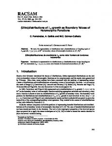
real and/or reactive power that can be added before the system experiences voltage collapse, with the distance to the SNBP being a quick indicator of stability margin. The phenomenon of the SNBP can be explained using an example of a two-bus dc system, consisting of a constant voltage source V0 (1 pu) connected to a real-power load P, by a branch of resistance R = 0.1 pu. The power-balance equation at the load bus is given by, V0 V P R V
(2.1)
where V is the voltage at the load bus. The two solutions of (2.1) are plotted against the real-power load in the system in Figure 2.1. It is seen that for all P < 2.5 pu, two voltage solutions exist for the system, of which the higher solution is the operable solution and the lower solution is the inoperable solution. At the SNBP when P = 2.5, the two solutions coalesce and finally beyond the SNBP (P>2.5), no solution exists for the problem.
Figure 2.1 Solutions of a two-bus dc system vs. load 11
Thus, the SNBP of a system is the point at which the operable and the inoperable solutions coalesce and beyond that point no solution exists for the given problem [41]. For a power system, the SNBP can be denoted by the maximum load-scaling parameter λ, for which the power-flow problem has a stable operating point. It is not necessary to scale all loads uniformly when determining the SNBP, a certain pre-defined direction of change can be chosen. It has been shown that no dynamics are required to be modeled in order to obtain the SNBP of a system and that the small signal voltage stability limit depends only on the steady-state characteristics of the system [47] - [49]. It has been shown that the right eigenvector of the Jacobian matrix at the SNBP gives the initial direction of dynamic voltage collapse while the left eigenvector can be used for monitoring of voltage collapse and taking corrective actions to avoid it [50]. When the loadscaling parameter is at its SNBP value, one of the eigenvalues of the Jacobian matrix becomes zero and thus the Jacobian matrix becomes singular. Since the NewtonRaphson power-flow method requires the inversion of the Jacobian in order to solve the problem, adaptations such as continuation methods have been used as stabilizers [42]. Some well-researched methods of estimating the SNBP will be discussed in this section.
2.1.1
Continuation power flow
The method used in most PF applications to estimate the SNBP is the continuation power flow (CPF), which is a NR-based method [43], [44]. The idea of the CPF is to 12
follow the characteristic power-voltage (PV) curve of the power system. Starting from a known solution on the PV curve, the load in the system is increased and a continuum of power flow solutions is found until the SNBP is reached [44]. The primary advantage of the CPF is that it slightly reformulates the power-flow problem using an additional parameter that models the load increase, such that the modified Jacobian in the problem is not singular even at the SNBP. The known solution is used to estimate a subsequent solution corresponding to a different value of the continuation parameter using a tangent predictor. The estimate is then corrected in the “corrector” step to obtain the accurate solution using Newton-Raphson. The details of the CPF are described in this section. The power-balance equations corresponding to the ith bus are originally given by (2.2), n
0 PGi PLi ViVk y ik cos( i k vik ) k 1
n
0 QGi QLi ViVk y ik sin( i k vik )
(2.2)
k 1
where Viejδi, Vkejδk are the voltages at bus i and bus k, respectively, yikejvik is the (i,k)th element of the bus admittance matrix, PLi and QLi are the real and reactive loads and PGi and QGi are the real and reactive generations at bus i respectively. These equations can be modified to (2.4) using a load increment parameter defined by (2.3),
0 critical
(2.3)
13
n
0 PGi 0 (1 k Gi ) PLi0 k Li S base cos i ViVk y ik cos( i k vik ) k 1
n
0 QGi QLi0 k Li S base sin i ViVk y ik sin( i k vik )
(2.4)
k 1
where PLi0 and QLi0 are the original real and reactive loads at bus i, PGi0 is the original real generation at bus i, kLi and kGi denote the rate of load change and generation change at bus i respectively as λ changes, ψi represents the power factor of the load change at bus i and SΔbase is the apparent power that provides an appropriate scaling of λ. The different kLi, kGi and ψi allow the power at each bus to be changed independently. The base solution is used to predict the next solution by obtaining a suitable step along the tangent to the solution path. The tangent is calculated by taking a derivative of (2.4) along with an additional equation to choose the magnitude, typically 1.0, of one of the tangent vector components. Thus the tangent vector is obtained as given by (2.5), F d FV dV F d 0 F
FV ek
d F 0 dV 1 d
(2.5)
where δ denotes the N x 1 (N is the number of buses in the system) vector of bus voltage angles, V denotes the N x 1 vector of bus voltage magnitudes, 0 denotes a 2N x 1 vector of zeros. The variable Fδ is a 2N x N matrix of the partial derivatives of (2.4) with respect to the bus voltage angles i.e. δ. The variable FV is a 2N x N matrix of the partial derivatives of (2.4) with respect to the bus voltage magnitudes i.e. V. The combined matrix [Fδ FV], a square matrix of dimension 2N x 2N, is the same as the Jacobian
14
matrix of the original power-flow equations (given by (2.2)). The variable Fλ is a 2N x1 vector of the partial derivatives of (2.4) with respect to λ. The variable ek is a 1 x (2N+1) row vector, with only the kth element being one and all others being zero. The tangent vector obtained by solving (2.5) is a (2N+1) x 1 column vector. The matrix in (2.5) is guaranteed to be non-singular even at the SNBP due to the additional λ parameter. When the high voltage path of the P-V curve is being traced (i.e. the load is increasing), +1.0 should be used in (2.5), while -1.0 should be used when tracing the low-voltage solution path. The prediction of the next solution is then made using (2.6) where σ indicates the step size which can be varied as the continuation process progresses and the ‘*’ terms are the predicted solution for the next step.
* d * V V dV * d
(2.6)
x V
The corrector step then involves solving (2.4) (using Newton-Raphson method) such that xk, the continuation parameter has the value xk* obtained from step (2.6). The load parameter λ is the typical choice for the continuation parameter in the CPF at normal loading conditions when the voltages are relatively slow-changing, whereas at heavily loaded conditions, the voltage magnitudes and angles experience a faster change and hence can be better continuation parameters. The SNBP is then detected
15
when dλ from (2.5) becomes zero while traversing the stable P-V curve and it becomes negative after the SNBP. Weak buses can also be determined based on the buses with the highest change in voltage as the load parameter changes. One of the important uses of the CPF is to estimate the available transfer capabilities (ATCs) for critical interfaces. ATC is the available capacity to transfer power over a given interface over and above the existing power flow across the interface, while obeying the restriction that there are no voltage limit violations, thermal overloads, voltage collapse or transient stability issues for a set of faults [60], [61]. As per the Federal Energy Regulatory Commission (FERC) requirements, the ATCs for key interfaces has to be made available on a publicly accessible Open Access Same-time Information System (OASIS) [59]. Hence the CPF is a key part of the reliability studies conducted by all independent system operators (ISOs). For example, PJM Interconnection conducts voltage stability studies on key interfaces every day after the day-ahead scheduling is completed [62]. It also runs a “transfer limit calculator” every 4-5 minutes using the state estimator snapshot to establish the safe operating limits of critical interfaces [62]. Likewise, CAISO also performs day-ahead PV analysis for critical interfaces along with a real-time voltage stability analysis run every five minutes [63]. The computational complexity of the CPF is much higher than a simple NR PF since it requires solving a new PF problem at each step as one moves along the P-V
16
curve toward the SNBP [44]. This increase in the execution time may became problematic when the system size becomes large. 2.1.1.1 Further improvements and modifications to the CPF Significant research has been done in order to study and improve the accuracy and speed of the CPF. The CPF with an adaptive step size control using a convergence monitor was proposed in [53]. In this approach, the step-size calculated using the convergence monitor is compared with the step size obtained using the sensitivity of the reactive power generations and the voltages with respect to the continuation parameter and the smallest step size is chosen. Global geometric parameterization was used in [54] for the CPF without change of the continuation parameter. Further, the process was made faster by updating the Jacobian only after significant changes in the system are seen such as boundary conditions or topology changes. A local geometric parameter approach was used for the CPF in [55] which could be used to trace the entire P-V curve with a fixed step length. Amongst many other publications on the parameterization of the CPF, are [56] which proposed the use of arc length as a parameter, and [57] which proposed the use of real-power losses across one of the branches as a parameter. The drawbacks of global parameters such as arc length were demonstrated in [58]. Another approach to speeding up the CPF was proposed [66] using a system reduction technique where the largest elements of the tangent vector at a known operating point is used to determine the critical load clusters that are “strongly” connected to
17
generate independent systems. Furthermore, variables that suffer little change during any continuation step of the CPF are eliminated by fixing them at the last equilibrium value. However the partitioning techniques used for generating independent subsystems were shown to be inadequate, as the independent systems obtained at a particular loading level were not able to capture the system behavior for broad load variations [66]. The clustering technique could however be useful in identifying the critical area with respect to voltage stability. If the cluster does contain the critical bus, an index called Tangent Vector Index (TVI) which is the reciprocal of the largest entry in the tangent vector can be used to modify the predictor step-size and the process is continued until the TVI is lower than a certain threshold in order to quickly estimate the SNBP with a speed-up of about three times over the conventional CPF [66]. While the above proposed improvements still require multiple power-flow problems to be solved, it will be shown in chapter 3 that the HEPF-based methods proposed in this document can estimate the SNBP, as well as trace the P-V curve, by solving a single power-flow problem.
2.1.2
Other methods for SNBP estimation
Approaches other than the continuation method have also been investigated in order to estimate the SNBP, some of which will be briefly noted here. A summary of the point of collapse (POC) method of estimating the SNBP which calculates the point at which the Jacobian has a single zero eigenvalue with non-zero left and right eigenvectors is 18
presented in [67] where the corresponding right eigenvector can be used to detect the areas prone to voltage collapse and the left eigenvector can be used to compute an optimal control strategy to extend the SNBP. A predictor-corrector method was proposed in [65] in order to estimate the reactive power limit points with the maximum reactive power from any generator being voltagedependent. The predictor step was based on the sensitivities of the reactive power generation at points of VAr support to change in the loading parameter while the corrector step finds the point at which both the voltage is constrained to its specified value as well as the reactive power is constrained to its limit. Since the above methods do not involve solving multiple power-flow problems, they are expected to be faster than the CPF, however they do not trace the PV curve and hence convey less information. Optimization algorithms such as the genetic algorithm, particle swarm optimization and their variants have been used to detect the closest SNBP in [68] - [74] amongst others. These Optimal Power Flow (OPF) based methods maximize the loading parameter such that the power flow equations, generator reactive power limits are satisfied. In the standard form, the voltage magnitude and reactive power generation at the generator buses are allowed to vary between certain bounds in order to obtain the optimal solution, as opposed to the CPF where the voltage magnitude at the generator buses is kept fixed as long as the generator VARs are within limits. The equivalency of the OPF-
19
based methods and the CPF when certain optimality conditions are met is shown in [70], [75]. The optimization-based approaches are also computationally expensive as they involve solving nonlinear, non-convex optimization problems. Wide-area-measurement-based voltage stability analysis using modified coupled single-port models has been examined in [81]; while physical constraints such as VAr limits are not considered in that work, they are shown to be important. Many research papers focused on measurement-based voltage stability studies have been published, of which [64], [81] - [84] are only a few. Artificial neural network based methods of assessing voltage stability have been proposed in [76] - [80] amongst others. There are numerous ways to train the artificial neural network, while some focus on ensuring that the probability of failure is less than a certain value, others use the neural network to obtain certain stability indices to determine the proximity of the system to voltage collapse. One of the primary goals of these alternatives to continuation-based methods of assessing the steady-state voltage stability of a system is to reduce the computation time involved in the CPF. Trying to find efficient ways of estimating the maximum loading point of systems continues to remain a topic of interest. Additionally, the model-based approaches mentioned, use numerical techniques such as Newton-Raphson which can have convergence issues. The work presented in this document will use the HEPF to estimate the SNBP since it is theoretically guaranteed to obtain the operable solution to
20
the given nonlinear power-flow problem, if one exists [16], [17]. Another goal is to reduce the computational effort required in performing this analysis. 2.2 Network reduction methods A second focus of this research has been the application of the holomorphic embedding method to the network reduction problem. Because of network size and/or model/problem complexity, it is often necessary to obtain a reduced-order network model of a large, complicated systems in order to limit the computational effort needed to perform planning studies and make investment decisions. To this end, a variety of network reduction techniques have been developed in the past, of which the Ward reduction and its variants are the most widely used. With the available computation capacity, transmission networks are modelled in detail in most power system analysis studies; however the distribution systems are often represented at the point of interconnections as an aggregated injection obtained using Ward reduction (or one of its variants) or by estimation of the demand at that point from historical data. A short review of Ward-reduction methods is discussed next. Note: In the rest of this document, the terms “external buses/ external system/ external network” refer to the portion of the original system that was eliminated during the reduction and is not a part of the reduced network; while the term “internal buses” refers to the portion of the original system that was retained in the reduced network.
21
2.2.1
Ward reduction
In the traditional Ward reduction method, the nonlinear generation/load models at external buses are linearized as current injections at each external bus based on the given operating condition [85], [86]. The eliminated portion of the original network is then modeled as equivalent constant current injections at the boundary buses of the reduced network. The current injections at the external, boundary and internal buses calculated in the previous step, can be used to obtain the bus voltages as shown in (2.7).
I e Yee I Y b be I i
Yeb Ybb Yib
Ve Ybi Vb Yii Vi
(2.7)
By performing partial LU factorization, (2.7) can be modified to (2.8).
I e Lee I L b be I i
I
I Y Y Y 1Y bb be ee eb I Yib
U ee Ybi Yii
U eb I
Ve V b I Vi
(2.8)
Thus the boundary bus equivalent currents can be calculated by multiplying the LHS of (2.8) with the inverse of L as given in (2.9).
I b Lbe Lee1 I e I b' Ybb YbeYee1Yeb Ybi Vb Ii Yib Yii Vi Ii
(2.9)
Finally, the equivalent currents are converted to complex power injections using the voltages at the given operating condition.
22
The Ward-injection method, converts the external shunts to current injections prior to the procedure described above, so that only the series elements1 of the external network are used to obtain the branch parameters of the reduced network, thus representing only the base-case effects of the shunts [90]. The Ward-admittance method (or Kron reduction) on the other hand, models all external injections as shunts so that the current injections at the external buses are zero [90]. This approach however has the drawback that the shunts in the reduced network can become very large and these unusual values can affect the convergence of power-flow algorithms, particularly the decoupled algorithms [90]. Thus, the Ward-injection reduction method is preferable. Ward reduction assumes that the loads and generation in the external network remain at a fixed schedule of real and reactive power and that the voltage profile remains the same as in the base-case condition. Hence for operating conditions different from the base-case, the Ward reduction fails to model the change in losses accurately and fails to model the reactive power support (bus voltage control) from the external network accurately.
2.2.2
Other methods of network reduction
As an improvement, the extended Ward method accounts for reactive power support from the external network by creating a fictitious generator buses attached to each
1
The term “series elements” in this document refers to the non-shunt part of the network.
23
boundary bus, generators which do not generate any real power but instead provide reactive power support [87]. Another way to model the external reactive power support was proposed in the Radial Equivalent Independent (REI) method which aggregates the injection of the external buses to a fictitious REI node which is connected to the boundary buses by fictitious branches [88], [89]. A critical analysis of the above-mentioned reduction methods and their variants is described in [90] where the heavy dependency of these methods on the operating condition is pointed out. Kron reduction is another method used to analyze power systems with a focus on the voltage profiles of a few selected buses [91]. Buses with non-zero current injections which are not of interest are converted to shunt admittances and all these buses with zero current injections are then eliminated using Kron reduction. A comparison of the commonly used network reduction methods such as Ward reduction, Kron reduction and REI reduction is provided in [91] where it is shown that the performance of the methods varies with the extent of the change in operating condition, and is also system dependent. A novel method to improve the REI method has been proposed in [92] to better model the change in operating condition. It updates the REI equivalent obtained using the base-case operating condition by running a state estimation on the internal network and finding the mismatch on the boundary buses and thus can also account for topology changes in the network.
24
Bus aggregation techniques have also been used to produce reduced-order dc networks, such as [93] which divides the given system into zones and then uses power transfer distribution factors (PTDFs) in an overdetermined problem formulation to calculate equivalent-branch-susceptance parameters that best match the base-case interzonal power flows. The method was shown to have more accurate results for inter-zonal power flows than the Ward and REI equivalents even for operating conditions different from the base-case, along with being computationally more efficient. Bus aggregation technique is also used in [94] which uses the congestion profile of the original network to assign flow limits on to the reduced-order dc network. The results of an optimal power flow (OPF) performed on the reduced network show that while the congestion profile of the original network is retained, the LMPs obtained can have up to a 15% error for some of the cases examined [142]. Thus developing network equivalents which can more accurately model changes in operating conditions of the original network remains an area of interest, an issue we address in this work, particularly for developing more accurate representations of the distribution systems connected to an HV transmission system.
25
3 HEPF-BASED METHODS OF ESTIMATING THE SADDLE-NODE BIFURCATION POINT OF A SYSTEM Estimating the saddle-node bifurcation points of power systems and available transfer capabilities across critical interfaces is an important study performed during planning as well as in the operational realm. Predicting the SNBP of a power system has become more critical as the power-system loading has increased in many places without a concomitant increase in transmission resources. Since a Newton-Raphson power-flow method is inherently unstable near the SNBP, adaptations such as continuation methods have been used as stabilizers. Since the power-flow problem lies at the heart of the SNBP-estimation, HEPF can be used to advantage for this purpose as it is theoretically guaranteed to find the high-voltage solution to the power-flow problem, if one exists, up to the SNBP, provided sufficient precision is used and the conditions of Stahl’s theorem are satisfied by the equation set. In this chapter, four different HEPF-based methods to estimate the saddle-node bifurcation point of a power system, are proposed and compared in terms of accuracy as well as computational efficiency. The first step in developing a proper HEPF formulation is to render the PBE’s (originally non-holomorphic due to the presence of the complex conjugate operator) holomorphic. While there are an infinite number of ways of embedding the nonlinear nonholomorphic power-flow equations, three different formulations are explored for SNBP estimation: 26
a. Non-scalable formulation: This formulation represents the original PBE’s only at (embedding parameter) α = 1.0 and V(α) evaluated any other value of α is meaningless [40]. b. Uniform scaling formulation: The advantage of using this formulation [95] over previously published formulations ([16], [17], and [40]) is that the solution V(α), evaluated at any value of α = αk short of the SNBP, represents the bus voltages when all the loads and generation in the system are uniformly scaled. c. Direction-of-change scaling formulation: For most studies, it may not be desirable to scale all loads uniformly, but rather in a pre-defined direction of change. Using this formulation [95], the solution V(α), evaluated at any value of α = αk short of the SNBP, represents the bus voltages when the change in the loads and generation in the system are scaled in a uniform manner that is similar to the CPF. The last two formulations can be used to an advantage to estimate the SNBP without solving multiple power-flow problems. It can also be used to trace the high voltage path of PV curves by simply substituting different values of α in the solution V(α), without solving multiple nonlinear problems. 3.1 Formulation to scale all loads and generations uniformly Consider a general (N)-bus system consisting of a slack bus, called slack, a set m consisting of PQ buses, a set p consisting of PV buses which are not on VAr limits and 27
a set q consisting of PV buses that are on maximum/minimum VAr limits. The PBE for a PQ bus with a constant power load is given by,
S i* YikVk * Vi k 1 N
,i m
(3.1)
where Yik is the (i, k) element of the bus admittance matrix, and Si and Vi are the complex power injection and voltage at bus i, respectively. The traditional defining equations for a PV bus are given by (3.2) and (3.3).
N * * Pi ReVi Yik Vk , i p k 1
(3.2)
Vi Vi sp , i p
(3.3)
where Pi denotes the real power injection and Visp is the specified voltage magnitude at bus i. PV buses on VAr limits are treated similar to PQ buses with their reactive power generation fixed at the appropriate limit and the real power generation given by (3.2). It is possible to embed (3.1) - (3.3) in such a way that the solution obtained at different values of real α, represents the solution (if it exists) when the complex power injections at the load buses and real power at generation buses are scaled by a factor of α. It is necessary to have such a formulation in order to be able to estimate the SNBP of the system without having to solve a new PF problem at different loading conditions. The HEPF formulations published in the past, do not allow one to scale the load by a factor of α, since they solve the given power-flow problem only at α=1.0, because they are consistent with the power system equations only at α=1.0. Consider
28
the following set of holomorphically embedded equations, where (3.4) represents the PBE for PQ buses, (3.5) represents the voltage magnitude constraint for the slack bus, (3.6) represents the PBE for the PV buses, (3.7) represents the voltage magnitude constraint for the PV buses and (3.8) represents the PBE for PV buses on VAr limits, N
YikVk ( ) k 1
S i * , i m * Vi ( * )
(3.4)
Vi ( ) Vi sp , i slack N
Y V k 1
ik
k
( )
(3.5)
Pgi Pli j Qgi ( ) Qli Vi ( * ) *
, i p
2
Vi ( ).Vi ( * ) Vi sp , i p *
N
Y V k 1
ik
k
( )
(3.6) (3.7)
Pgi Pli j Qgi _ lt Qli Vi ( * ) *
, iq
(3.8)
where Pgi denotes the real-power generation, Pli denotes the real-power load, Qgi(α) denotes the reactive-power generation, Qli denotes the reactive-power load at bus i and Qgi_lt denotes the respective maximum/minimum VAr limit for a generator bus on maximum/minimum VAr limits. The real and reactive power injections at bus i are given by:
Pi Pgi Pli , i p
(3.9)
Qi Qgi ( ) Qli , i p
(3.10)
Using (3.9), (3.6) and (3.8) can be written as: N
Y k 1
ik
Vk ( )
Pi jQli jQgi ( ) Vi ( * ) *
, i p
29
(3.11)
N
Y V k 1
ik
k
( )
Pi jQli jQgi _ lt Vi ( * ) *
, i q
(3.12)
Since V(α) and Qgi (α) are holomorphic functions of the parameter α, they can be expressed as Maclaurin series given by:
V ( ) V [0] V [1] V [n]
n
Qgi ( ) Qgi [0] Qgi [1] Qgi [n]
n
(3.13)
where Qgi (α) is a real-valued series. Note that the variable V* in (3.4), (3.7), (3.11) and (3.12) is embedded with α* instead of α in order to ensure that the Cauchy-Riemann conditions are satisfied, thereby retaining the holomorphicity of the function. For this reason, it is important to keep in mind, that (3.4), (3.7), (3.11) and (3.12) represent the given power system only for real values of α [96]. The Maclaurin series for V*(α*) is given by:
V * ( * ) V *[0] V *[1] V *[n]
n
(3.14)
The proof that the series given by (3.13) is the Maclaurin series for the given formulation is derived in Appendix D. Equations (3.4), (3.5), (3.7), (3.11) and (3.12), represent a new formulation that allows the loads at all buses, and the real-power generation at PV buses, to be scaled by a factor of α. Note that in (3.11), only the reactive-power generation Qgi is written as a function of α instead of the net reactive-power injection Qi. This allows the reactive-power load to be scaled by a factor of α, while the variable value of reactivepower generation needed to maintain bus voltage control, is calculated from the power series. Also, in (3.12), Qgi_lt is not multiplied by α, since this is fixed for a bus on VAr limits
30
and the reactive power cannot be scaled with α. This is the only difference between the equation for PQ buses and that for PV buses on VAr limits. By substituting the series V(α), V*(α*) and Q(α) given by (3.13) and (3.14) into (3.4), (3.5), (3.7) (3.11) and (3.12), we obtain:
N
Yik Vk [0] Vk [1] Vk [2] 2 k 1
V [0] V [1] V [2] i
i
2
i
Vi sp , i slack
Y V [0] V [1] V [2] N
ik
k 1
k
k
S i * , i m Vi* [0] Vi* [1] Vi* [2] 2
k
2
(3.16)
Pi jQli j Qgi [0] Qgi [1] Qgi [2] 2 , i p Vi*[0] Vi* [1] Vi*[2] 2
V [0] V [1] V [2] i
i
Vi
sp 2
2
i
k 1
(3.18)
,i p
Y V [0] V [1] V [2] ik
(3.17)
. Vi* [0] Vi* [1] Vi* [2] 2
N
k
k
k
2
(3.15)
V
i
Pi jQli jQgi _ lt *
[0] Vi* [1] Vi* [2] 2
,iq
(3.19)
Since it is required that (3.15) - (3.19) hold true for any value of α, the coefficients of the respective powers of α on both sides of the equations must be equal. In order to find the series coefficients that satisfy these equations, the inverse of the voltage power series on the RHS has to be represented as a power series. To achieve this, let the inverse of the voltage function V(α), be represented by another power series, W(α), defined by W(α)=W[0]+W[1]α+W[2]α2+… where the relationship between W(α) and V(α) is given by (3.20).
W ( )
1 V ( )
(3.20) 31
Thus equations (3.15)-(3.19) are now modified to:
Y V [0] V N
ik
k 1
k
k
[1] Vk [2] 2
(3.21)
S i Wi [0] Wi [1] Wi [2] , i m *
*
*
*
V [0] V [1] V [2] i
i
Y V N
ik
k 1
k
2
i
2
Vi sp , i slack
(3.22)
[0] V k [1] V k [2] 2
(3.23)
Pi jQli j Q gi [0] Q gi [1] Q gi [2] 2
W [0] W [1] W [2] , i p V [0] V [1] V [2] . V [0] V *
*
i
*
i
2
i
2
i
i
*
i
i
i
*
[1] Vi*[2] 2
2
Vi sp , i p
Y V [0] V [1] V [2] N
k 1
ik
k
k
k
2
(Pi jQli jQgi _ kt ). Wi [0] Wi [1] Wi [2] , i q *
*
*
(3.24)
(3.25)
2
In order to guarantee that the HEPF can find an operable solution (if one exists), it is critical to have the correct germ [17], [16], [20]. The germ is the solution obtained by solving the holomorphically embedded equations representing the PF problem at α=0. This extrapolation-capable formulation presented above, however, poses some challenges when calculating the germ. The system of equations to be solved for the germ is given by (3.26.a)-(3.26.d).
32
N
Y k 1
ik
N
Y k 1
ik
Vk [0] 0 , i m Vk [0]
(a)
jQ gi [0] *
Vi [0]
, i p
(b)
2 V [0] V * [0] Vi sp , i p i i Vi [0] Vi sp , i slack N
Y k 1
ik
Vk [0]
jQ gi _ lt *
Vi [0]
(c )
(3.26)
(d )
, iq
( e)
Note that (3.26.b) and (3.26.c), representing the PBE and the voltage magnitude constraints for PV buses and (3.26.e) representing the PBE for PV buses on VAr limits, cause the system of equations that need to be solved to obtain the germ to be nonlinear. Since the NR is known to have good convergence properties for lightly loaded systems and the germ represents the solution for a no-load, no-real-power-generation scenario, this germ can be obtained by using the NR for this special case, and it may be a better choice in order to minimize the computational time required in finding the germ. However, it is possible, that NR might not give the right germ; it could converge to the lowvoltage solution for this lightly-loaded problem (the only loads are the shunts). However, if one wants an algorithm that is guaranteed to find the correct germ, the HEPF can be applied to solve (3.26) as explained in the following sub-section 3.1.1.
3.1.1
Calculating the germ using HEPF
The nonlinear problem given by (3.26) can be solved using the HEPF, wherein the voltages and reactive powers at α=0 can be represented as different Maclaurin series of the complex embedding parameter β, given by (3.27) - (3.31), 33
N
Y
V
ik trans k _ 0
k 1
( ) Yi shuntVi _ 0 ( ) , i m
(3.27)
Vi _ 0 ( ) 1 (Vi sp 1) , i slack N
Y k 1
V
ik trans k _ 0
( )
jQgi _ 0 ( ) Vi _ 0 ( * ) *
* Vi _ 0 ( )Vi _ 0 ( * ) 1 Vi sp N
Y k 1
Vk _ 0 ( )
ik trans
(3.28)
2
1 , i p
j Qgi _ lt Vi _ 0 ( * ) *
Yi shuntVi _ 0 ( ) , i p
(3.29) (3.30)
Yi shuntVi _ 0 ( ) , i q
(3.31)
where Yik trans corresponds to the “non-shunt-branch” part of the admittance matrix, shunt
Yi
corresponds to the shunt part of the admittance matrix, Vi_0(=1) and Qgi_0(=1),
represent the voltage and PV-bus-reactive-power injections under no-load conditions, respectively. The set of equations to obtain the germ for the above formulation is given by (3.32). N
Y
ik trans
Vk _ 0 [0] 0 , i m, q
ik trans
Vk _ 0 [0]
k 1 N
Y k 1
jQi _ 0 [0] *
Vi _ 0 [0]
(a) ,i p
(b)
Vi _ 0 [0].Vi *_ 0 [0] 1, i p
(3.32)
(c )
Vi _ 0 [0] 1, i slack
(d )
Since only the non-shunt branches are included in Yik trans, the sum of all off-diagonal elements in any row is equal to the negative of the diagonal element. Thus a voltage magnitude of 1.0 pu and a voltage angle of 0° for all of the PQ buses is consistent with (3.32.a). Equations (3.32.c) and (3.32.d), are likewise satisfied when voltage germs for the PV buses and the slack bus are assumed to be 1.0 pu. Finally, (3.32.b) must be 34
solved for the generator reactive power injection at = 0. From inspection, we see that the reactive-power germ is 0.0. Thus, the germ for this formulation can be obtained through observation rather than calculation. Using this germ, a recursive relation can be developed to find the remaining terms of the power series by equating the coefficients of the same powers of β on both sides of (3.27) - (3.31). Equating the coefficients of the same powers of β on both sides of (3.27), (3.28), (3.29) and (3.31), we obtain (3.33), (3.34), (3.36) and (3.37). N
Y
Vk _ 0 [n] Yi shuntVi _ 0 [n 1], i m
ik trans
k 1
Vi _ 0 [n] n 0 n1 (Vi sp 1), i slack
(3.33) (3.34)
where δni is the Kronecker delta, defined by (3.35).
1 , if n i ni 0 , otherwise N
Y k 1
ik trans
(3.35)
Vk _ 0 [n] jQgi _ 0 [n]
n 1 * j Qgi _ 0 [k ]Wi _ 0 [n k ] Yi shuntVi _ 0 [n 1], i p k 1 N
Y k 1
ik trans
Vk _ 0 [n] jQgi _ ltWi*_ 0 [n 1] Yi shuntVi _ 0 [n 1], i q
(3.36)
(3.37)
Equating the coefficients of the powers of β on both sides of (3.30) yields (3.39), where Vi re[n] represents nth coefficient of the real part of the voltage power series from the voltage-magnitude constraint. The notation δni, as defined in (3.35), may be used to write a generalized expression to evaluate Vi re[n]. The derivation of Vi re[n], ip, for an arbitrary value of n is given in (3.38). 35
Vi _ 0 [0]Vi _ 0 [0] 1 Vi _ 0 [0] 1 ( germ ) *
2
Vi _ 0 [0]Vi _ 0 [1] Vi _ 0 [1]Vi _ 0 [0] Vi sp_ 0 1 *
*
2
Vi _ 0 [1] Vi _ 0 [1] 2Vi _ 0 re [1] Vi sp_ 0 1 *
(3.38)
Vi _ 0 [0]Vi _ 0 [n ] Vi _ 0 [1]Vi _ 0 [n 1] Vi _ 0 [n 1]Vi _ 0 [1] Vi _ 0 [n]Vi _ 0 [0 ] 0 *
*
*
n 1
*
Vi _ 0 [n ] Vi _ 0 [n] 2Vi _ 0 re [n] Vi _ 0 [k ]Vi _ 0 [n k ] *
*
k 1
2
Vi _ 0 re [n] n 0 n1
Vi sp_ 0 1 2
1 n 1 Vi _ 0 [k ]Vi*_ 0 [n k ] 2 k 1
(3.39)
Equations (3.33), (3.34), (3.36), (3.37) and (3.39) are solved to obtain the remaining terms of the power series. Once a sufficient number of terms are obtained to meet the desired convergence tolerance, Padé approximants can be used to obtain the converged voltages and PV-bus-generated reactive powers for the germ.
3.1.2
Recurrence relations for the scalable form
Once the germ is obtained, the recursive relations to find the remaining terms of the power series, are obtained by equating the coefficients of same powers of α on both sides of equations (3.4), (3.5), (3.7), (3.11) and (3.12). Equations (3.40) and (3.41) provide the recurrence relations for the PQ buses and the slack bus respectively. N
Y k 1
ik
Vk [n] S i*Wi* [n 1], i m
Vi [n] 0, n 0
(3.40)
i slack
(3.41)
The recurrence relation for the PBE of PV buses is obtained as: 36
n * * Y V [ n ] ( P jQ ) W [ n 1 ] j Qgi [k ]Wi [n k ] ik k i li i k 1 k 0 N
(3.42)
Equation (3.42) can be further simplified to: N
Y k 1
Vk [n] ( Pi jQli )Wi [n 1] *
ik
n 1 * * * j Qgi [k ]Wi [n k ] Qgi [n]Wi [0] Qgi [0]Wi [n] k 1
(3.43)
The unknowns Qgi[n] and Wi[n] can be moved to the LHS, leaving all known quantities on the RHS to obtain: N
Y k 1
ik
Vk [n] jQgi [n]Wi [0] jQgi [0]Wi [n] *
*
(3.44)
n 1 * ( Pi jQli )Wi [n 1] j Qgi [k ]Wi [n k ] k 1 *
Notice that in the above equation, a new unknown, W[n], is introduced. In order to calculate the coefficients of the inverse power series, W[n], both sides of (3.20) are multiplied by V(α).
W ( )V ( ) 1
W [0] W [1] W [2]
2
V [0] V [1] V [2] 2 1
(3.45)
By equating the coefficients of the same powers of α on both sides of (3.45) a relation between W[n] and V[n] is obtained as given in (3.46). 1 V [0] W [1]V [0] W [0]V [1] 0 W [0]
(3.46) n 1
W [0]V [n] V [0]W [n] W [k ]V [n k ], n 1 k 1
37
Equating the coefficients of same powers of α, on both sides of the embedded voltage magnitude constraint equation given by (3.18), we obtain:
Vi [0]Vi [n ] Vi [n]Vi [0 ] Vi [1]Vi [n 1] ... Vi [n 1]Vi [1] *
*
*
n 1
*
Vi [k ]Vi [n k ], *
n 1
(3.47)
k 1
Note that all the quantities on the RHS of (3.47) are known. The recurrence relation for PV buses on VAr limits is obtained as: N
Y
ik
k 1
N
Vk [n] ( Pi jQli )Wi [n 1] jQgi _ lt .Wi [n] *
*
Yik Vk [n] jQgi _ lt .Wi [n] ( Pi jQli )Wi [n 1] *
*
(3.48)
k 1
Note that in (3.48) also, there is an extra unknown W[n], and thus an additional equation given by (3.46) needs to be added to the system of equations for PV buses on VAr limits in order to ensure that the problem is not under-determined. The system of linear equations (3.40), (3.41), (3.44), and (3.46)-(3.48) represent the recurrence relations for the formulation given by (3.4), (3.5), (3.7), (3.11) and (3.12). It is important to keep in mind that Qgi(α) is a purely real series. In order to obtain the power series coefficients using a single linear matrix equation, the unknowns need to be split into real and imaginary parts. Since the power series resulting from solving these recurrence relationships will only converge within its radius of convergence, Padé approximants are used to evaluate these series everywhere in the function’s domain, including where the series is non-
38
convergent. A Padé approximant is a rational-function (ratio of two polynomials) approximation to a power series that can yield a more accurate approximation to the defining function than the truncated series of the same length. A common Padé approximant notation to indicate that the degree of the numerator polynomial is L and the degree of the denominator polynomial is M, is [L/M]f(α), given in (3.49).
f ( ) [ L/M ] f ( )
a0 a1 aL L b0 b1 bM M
(3.49)
The matrix method used in this work for finding the rational approximant [22] is straight forward and involves solving a dense set of linear equations of dimension M and then a forward substitution through a dense lower triangular matrix of dimension L+1. The procedure for calculation and some key properties are described in detail in section 5.1 of this work. A diagonal Padé approximant for a series with a finite number of terms can be taken to be a rational approximant whose numerator and denominator polynomial degrees are equal (i.e., L=M). If the difference between the degree of the numerator and denominator polynomial is 1, (i.e., |L-M|=1), it is said to be a near-diagonal Padé approximant. Since the diagonal or near-diagonal Padé approximant is the maximal analytic continuation of the given power series [20], its value for any α within the function’s domain is guaranteed to be the HV solution for the above embedding with the germ defined above, provided the conditions of Stahl’s theorem are satisfied [20], [21]. Note that once the Padé approximants for the voltages are obtained, the SNBP may be found by varying α in the Padé approximants (not re-solving the PF 39
problem), using a binary search approach, until the boundary is reached at which the Padé approximant no longer obeys the PBE’s, provide a sufficient number of power series terms has been calculated. This point is the boundary of the function’s domain. Thus, this method may be viewed as a curve-tracing of the P-V curve for a system. It is important to point out that it is not necessary to evaluate the Padé approximants for all buses in order to check for convergence, but need be done only for a few arbitrarily chosen buses. The sequence of diagonal Padé approximants will have converged when the solution is reached; however, if there is no solution to the given problem, the Padé approximants will oscillate. If the given loading on the system is too low, the solution at α=1.0 may converge with very few terms in the power series. However, care must be taken to ensure that a sufficient number of terms is included so that an accurate solution is obtained at higher values of α, especially near the SNBP. 3.2 Non-scalable formulation While the germ calculation for the formulation presented in Section 3.1 requires solving a nonlinear problem, this section will present a non-extrapolating formulation whose germ may be found by inspection. One of the ways to holomorphically embed (3.1) - (3.3) is given by (3.49) - (3.53) where Yik trans corresponds to the “non-shuntbranch” part of the admittance matrix and Yi shunt corresponds to the shunt part of the admittance matrix [17], [40]. Since this formulation is non-extrapolating and is valid at 40
only α=1.0, (3.50) can be used to represent PV buses on VAr limits as well, by setting the reactive power generation to be at its appropriate limit. S i * Yik transVk ( ) * * Yi shuntVi ( ) , i m Vi ( ) k 1
(3.50)
Vi ( ) 1 (Vi sp 1) , i slack
(3.51)
N
N
Y k 1
V ( )
ik trans k
Pi jQi ( ) Yi shuntVi ( ) , i p * Vi ( * )
* Vi ( ) Vi ( * ) 1 Vi sp
2
1, i p
(3.52) (3.53)
The germ for this method is 1.0 for all the voltage series and zero for the reactive power series. Once the germ is obtained, the approach for obtaining the solution for this formulation is very similar to that presented in Section 3.1.1. It should be mentioned that this formulation not only provides an obvious germ, but also is in general a bit more advantageous in terms of numerical stability and precision [106]. This is because by not including the shunts in the no-load case, the magnitudes of the voltages do not vary as much when going from α=0 to α=1.0, and thus the Padé approximants behave slightly better numerically in general [96]. A drawback of the above formulation is that it represents the given power system only at α=1.0 and has no meaningful interpretation at any other value of α. Since Yi shunt is also multiplied by α, at any value of α≠1, the solution corresponds to a network whose shunt-branch parameters differ from those of the original network. Also, the voltage magnitude constraints, embedded as given in (3.51) and (3.53) will hold true only at α=1.0. For any other value of α, the voltage magnitude constraints for the PV buses and the slack
41
bus will not be obeyed. However, because the HEPF is theoretically guaranteed to converge to the HV solution (provided sufficient precision is used), this formulation can be used to calculate the SNBP using a binary search approach. This involves solving multiple PF problems and is of the order of complexity of the CPF, where complexity here is taken as the number of PF’s that must be solved. The computational complexity of the method proposed in Section 3.1 is much less than that of the repeated solution approach proposed here, since for that method, only the Padé approximants for the voltages must be evaluated until the function’s domain boundary is reached, which is indicated by high bus-power mismatches. 3.3 Using the roots of Padé approximants to estimate the SNBP The power series obtained may or may not converge depending on the value of α, i.e., for various loading conditions, even though a solution for the PF problem exists. The radius of convergence of the power series is determined by the closest singularity of the function to the origin [97]. Since the full solution V(α) is an algebraic curve, it has no poles; therefore the only singularities are its branch points on the α-plane (i.e., points where one or more branches coincide) [98]. The first singularity encountered along the real axis is precisely the bifurcation point that we seek [96]. However, in general, other branch points on the complex α-plane may be closer to α=0 [99]. In that case, the power series has a reduced convergence radius, and that is why Padé approximants are needed. If the point of interest (given the loading condition) is outside the radius of convergence, then the voltage series will diverge. The series therefore needs 42
to be ‘redefined’ such that a converged solution is obtained for all loading levels where a solution exists. The sequence of near-diagonal Padé approximants, proven to be the maximal analytic continuation of the power series by Stahl’s theorem [20], can be used to extend the convergence region of the power series over the domain of the function. There are several ways to calculate the Padé approximant and one commonly used is the matrix method, which is well-described in [22] and has been summarized in Section 5.1 of this report. A common Padé approximant notation is to use L as the degree of the numerator polynomial and M as the degree of the denominator polynomial. Though the matrix method described in [22] allows the calculation of a rational approximant of an arbitrary degree, Stahl’s theory [100] indicates that the close-to-diagonal Padé approximants yields the best accuracy when evaluating the power series outside its radius of convergence. Stahl’s work ([20], [21]), originated from Nuttall’s work [98], which proved that the poles of the close-to-diagonal Padé approximant accumulate on Stahl’s compact set. When a scaling formulation is used, the distance from the origin to the closest realvalued pole of the Padé approximant of the voltage power series gives the load-scaling value at the SNBP. The zeros of the Padé approximant accumulate in a manner similar to that of the poles; therefore the smallest real-valued zero or the smallest real-valued pole of the Padé approximant can be used to determine the proximity of the system to its SNBP. Some interesting results on the complexity of these poles and zeros have been
43
shown in [99]. While the SNBP can only be precisely obtained if computing the power series with an infinite number of terms and infinite precision, promising numerical results, given in sections 3.5, 3.6 and 3.8, show that the method works well for predicting the SNBP with a reasonable number of terms and finite precision. 3.4 The sigma methods The method described in this section to calculate the SNBP of a system is based on calculating a set of complex-valued ‘σ’ indices proposed in [101]. The idea behind the method is to develop a two-bus equivalent system for each node of the power system spanning that node and the slack bus, an equivalent that preserves only the slack bus voltage and the voltage at the retained bus. It is a local nonlinear equivalent at each node. The parameters for this proposed reduced equivalent are calculated to be consistent with the simple two-bus system comprised of a slack bus and a PQ bus as shown in Figure 3.1, where Z is the line impedance, S is the complex-power injection at the PQ bus (and hence P will be negative for real-power loads), V0 is the slack bus voltage and V is the PQ bus voltage. This section will describe the derivation of the σ indices, starting with a two-bus example [101].
Figure 3.1 Two-bus system diagram The power balance equation for the PQ bus in Figure 3.1, given by (3.54), can be 44
re-arranged to obtain (3.55), V V0 S* * Z V
(3.54)
U*
(3.55)
U 1
where U=V/V0 is the normalized voltage and σ is defined as:
ZS * V0
(3.56)
2
The roots of (3.55) which is a quadratic equation, are,
U
1 1 R I2 j I 2 4
(3.57)
where σI and σR are the imaginary and real parts of σ, respectively. If the slack bus voltage magnitude is assumed to be controlled at 1.0 pu, the two roots represent the high- and low-voltage solutions for the given two-bus network. The two solutions meet at the point at which the radicand becomes zero, the SNBP. For the high-voltage solution to exist in a two-bus system, it is necessary that the radicand in (3.57) be positive. Thus the condition to ensure that the two-bus system is short of or at its static voltage collapse point, called the ‘σ condition’, is given by: 1 R I2 0 4
(3.58)
For a multi-bus system, [101] proposed to find, for all system buses, two-bus equivalents spanning the slack bus and bus of interest, structurally equivalent to Figure 3.1, where the PQ bus power injection is the native injection at this bus in the full network. One immediately sees a problem when trying to map a voltage-preserving two-bus 45
equivalent (described below) onto the structure of Figure 3.1: In a realistic system model, normalized bus voltages with real parts less than 0.5 are common, but cannot occur for the high voltage solution in a two-bus system (assuming the slack bus voltage angle is 0°) as shown in (3.57). (In fact, the low voltage solution for the two-bus equivalent constructed below (low voltage solution from (3.57)) corresponds to the high voltage solution of the full network for cases when the real part of the normalized voltage is below 0.5.) Because [101] does not appear to recognize this incompatibility, nor recognize that taking the low voltage solution would have resolved this incompatibility, their theory leads to erroneous predictions. Two different ways of extending the σ equivalent to calculate the equivalent parameters of this two-bus equivalent and the proximity to voltage collapse for a general (N+1)-bus system are proposed in sub-sections 3.4.1 and 3.4.2 respectively. The ‘σ condition’ can be used to reasonably estimate the SNBP for multi-bus systems, but not in the straightforward way published in [101], as will be discussed at the end of this section.
3.4.1
Non-extrapolating sigma method
The method, given in [101], to estimate the voltage stability margin for a system, is an extension of the two-bus derivation to a general (N+1)-bus system. The normalized voltages at all buses in a full system model solution can be calculated using HEM, as power series of the embedding parameter ‘α’, given by U(α). A two-bus equivalent may 46
be constructed, and the σ index may then be obtained as a series of α, using (3.59) (which is structurally identical to (3.55)). U i ( ) 1
i ( ) U i* ( * )
(3.59)
V ( ) where U i ( ) i sp Vslack
and where Vi() represents the bus i voltage series and i() is the two-bus-model equivalent parameter to be determined. Multiplying both sides of (3.59) by Ui*(α*) yields:
U i ( )U i* ( * ) U i* ( * ) i ( )
(3.60)
Solving this for the power series σi(α) yields,
i ( ) U i ( )U i* ( * ) U i* ( * )
(3.61)
where σi(α)= σi[0]+ σi[1]α+ σi[2]α2 + …. By equating the constant terms on both sides of (3.61), we obtain, U i [0]U i*[0] U i*[0]
(3.62)
U i*[0](U i [0] 1) 0
Thus the germ corresponding to the high-voltage solution, must be Ui[0]=1.0, i.e., Vi[0]=Vslack. Equating higher powers of α on both sides of (3.61), the terms can be obtained as: n
i [n 1] U i [k ]U i*[n k ] U i*[n], n 1
(3.63)
k 0
Note that (3.62) implies that (3.61) in its given form, is valid only if the voltage germ for the PF problem is Vslack for the high voltage solution, which is not generally true for the extrapolation formulation given in Section 3.1. Such a germ is obtained for 47
the formulation given by (3.49) - (3.53); however this formulation cannot be used for extrapolation, which is problematic for the purposes here since the objective when using (3.61) is to increase (extrapolate) until the condition of (3.58) is violated. A modification to (3.61), which would allow extrapolation of α, is given in Section 3.4.2.
3.4.2
Extrapolating sigma method
If (3.59) is viewed as the mathematical analog of a two-bus equivalent of the original system reduced to a slack bus and bus of interest, then such an approximate equivalent might be used to predict the SNBP by scaling α until the sigma condition is violated [101]; however (3.59), in its present embedding, is valid for extrapolation to the SNBP only for voltage series obtained from HE formulations that allow α extrapolation and where the germ for the voltages is 1.0. For the formulation presented in Section 3.1 which allows extrapolation of α, the voltage germs are not necessarily 1.0 pu for practical systems. Hence (3.59) is only strictly valid for = 1.0 and extrapolation is approximate. We can modify (3.59) for use with the proposed extrapolation formulation, where the voltage germ is not 1.0. This can be done by eliminating α from the second term on the RHS of (3.59) as follows: U i ( ) 1
i ( ) U i* ( * )
(3.64)
Thus the equation for σi(α) can be obtained as:
48
U i ( )U i* ( * ) U i* ( * ) i ( )
(3.65)
i ( ) U i ( )U i* ( * ) U i* ( * ) The value of [0] for this formulation is obtained as:
i [0] Ui [0]Ui*[0] U i*[0]
(3.66)
The [n] terms in the modified formulation are given by: n
i [n] U i [k ]U i*[n k ] U i*[n]
(3.67)
k 0
Thus σi(α) can now be used as the parameter of an approximate two-bus equivalent network at different values of α, up to the SNBP. It is stated in [101] that the σ indices for all buses can be plotted to obtain a graphical measure of the proximity to voltage collapse as well as to identify the weak nodes. In other words, if a parabola is plotted as defined by the expression in (3.58), the distance from the σ indices in the plane to the surface of the parabola, can be used to estimate the distance from the SNBP, and the buses whose σ indices are closer to the surface are the weak buses. Typically, modal analysis is performed to determine the weak buses of a system. Modal analysis involves calculating the eigenvalues of the portion of the reduced Jacobian that retains only the Q-V relationships and determining the buses that have the highest participation factors in the critical modes with smallest eigenvalues [114] and is described in more detail in section 3.4.3. However, it will be shown that the sigma condition proposed in [101] will not produce reliable results and that a modified requirement can be used to produce a tight upper bound on the SNBP. Further,
49
theoretically there is no relationship between the buses judged to be weak using σ indices and the weak buses obtained using traditional modal analysis. Equation (3.65) can be split into real and imaginary parts to obtain: ( ) U ( )U * ( * ) U * ( * )
R ( ) U R ( )
U 2
I
( )
2
(3.68)
U R ( )
I ( ) U I ( )
where UR and UI are the real and imaginary parts of the normalized bus voltages, respectively, obtained using the full-model. The expression for σR(α) and σI(α) from (3.68) can be substituted into the expression given by (3.58), to obtain (3.69)
0.25 U ( ) U ( ) 0.25 U ( ) U ( ) U ( ) 0.5
0.25 R ( ) I ( )
2
2
R
2
I
U R ( ) U I ( )
2
R
2
(3.69)
R
2
R
Thus, it is seen from (3.69), the proximity of the ‘σ condition’ to zero, is equivalent to the proximity of the real part of the normalized bus voltage to 0.5. For a simple twobus (non-equivalent) system, indeed the real part of the normalized voltage is 0.5 at the SNBP and hence the proximity of the σ condition to zero is an indicator of the proximity to SNBP. However, for a multi-bus system (and hence its proper two-bus equivalent), this is not true and consequently, the magnitude of the σ condition is not a measure of closeness to the SNBP, but measures closeness to the point where the alternative root of (3.57) should be selected. Nor is the radicand of (3.57) approaching zero a reliable indicator of a weak bus as claimed in [101]; however, the buses whose σ condition first
50
approach zero as the system load is increased, have larger phase angles, which cause the real part of the normalized voltage to drop below 0.5. Consequently, the radicand approaching zero is not a measure of closeness to the SNBP, with a caveat described at the end of this section. Further, given this physical interpretation of the σ condition, and numerical results (from [140]), the buses closest to violating the σ condition do not necessarily correspond to the weak bus(es) of the system as determined in [114]. Hence, it is not clear that this approach can be used to obtain insights about the strength of a bus as claimed in [101], [95] without further research. The inadequacy of the proposed approach for estimating the SNBP when the system loading is lower than that at the SNBP loading, will be demonstrated numerically using the IEEE 118-bus system. The SNBP of this system occurs when all injections are multiplied by 3.18, i.e., at α = 3.18 (provided a scalable formulation is used), as obtained from MATPOWER [102]. The complex σ indices at α = 1.88 are plotted for all the buses on a two-dimensional plane as recommended in [101], and shown in the left plot of Figure 3.2. At α = 1.88 which corresponds to 60% of the maximum allowable loadscaling factor, some of the σ indices are very close to the surface of the parabola, i.e., limit imposed by the σ condition as shown in Figure 3.2. This occurs because some of the normalized bus voltages have real parts very close to 0.5, which causes the expressions in (3.58) and (3.69) to have very small numerical values for these buses.
51
Figure 3.2 Plot of σI vs. σR at α = 1.88 and α = 3.1 for the IEEE-118 bus system As the system loading increases further, the real part of the normalized voltage for the buses that were close to the surface at α = 1.88, decreases below 0.5, and hence the numerical value of the expression in (3.58) increases, causing the σ indices for these buses to move away from the surface of the parabola. This behavior is shown in the right plot of Figure 3.2, where the σ indices are plotted at α = 3.1, a point much closer to the SNBP. This behavior is further confirmed by plotting the σ condition expression against α as shown in Figure 3.3 for the first 10 buses (based on the native bus numbering) of the 118-bus system. It is seen that some of the buses come very close to violating the σ condition as α increases, far before the SNBP is reached, and then start increasing in value again, which is in agreement with the behavior shown in Figure 3.2. Such behavior, where the σ indices for some of the buses approach the parabola surface as the load
52
increases and then move away from the surface with further increase in the system load, has also been observed in radial systems with only PQ loads and thus it is not an effect of the complexity of the system.
Figure 3.3 Plot of σ condition vs. α for the IEEE-118 bus system If one searches for the point at which the σ condition is nearly satisfied (near zero), one will find that to occur for different buses at loading conditions well below the SNBP, and using the proximity of the σ condition to zero to estimate closeness to the SNBP would yield misleading and inconsistent conclusions; however, if one searches for the point where the σ condition becomes negative (which is theoretically impossible for voltage values short of the SNBP loading) using the Padé approximant of σ(α), one will obtain a reasonable estimate of the SNBP for the following reasons.
53
The Padé approximants of the bus voltages are found to be largely monotonic up to the SNBP, beyond which the voltage function no longer exists, and the evaluation of Padé approximants begins to oscillate wildly due to the poles and zeros of the approximants. The location of closest real-valued pole/zero when surveyed over all system bus voltages has been found to be a tight upper bound on the true SNBP [95]. Beyond the SNBP, the oscillations in the bus voltages (which have no physical interpretation) also appear as oscillations in the σ index. These oscillations inevitably lead to a σ condition which becomes negative just beyond the SNBP. Thus, the lowest load at which a negative value occurs in the σ condition, when surveyed over all buses in the system, is a good indicator of the location of the SNBP [95]. The search method proposed, can be thought of as being analogous (not equivalent) to solving multiple power-flow problems, at increasing load levels, while searching for the point at which the power-balance equations are not satisfied. When the modeled operating condition is even infinitesimally beyond the SNBP, the voltage functions do not exist but the Padé approximants of those voltage functions contain information that can be used to advantage. Beyond the SNBP the high power-balance mismatches are an indication that the system is now modeled to be beyond the SNBP. While it is true that the voltage function does not exist at that point, the unacceptable power-balance mismatches can nevertheless be used as an indirect indication of this non-existence. This will be demonstrated using the IEEE-14 bus system. The SNBP of the IEEE-14 bus system occurs when all loads and real-power
54
generations are scaled by 4.06, obtained using MATPOWER [102]. The Padé approximants of the voltage series with 41 terms in the series, if evaluated beyond α = 4.075 are seen to oscillate and do not represent the true voltages of the system. This is seen in Figure 3.4, in which the real part of the Padé approximants of voltage series are plotted against α, for the IEEE 14-bus system. The real parts of the near-real poles and zeros with the smallest real parts, which are the cause of these oscillations in the voltage Padé approximants, are listed in Table 3.1 for the non-slack buses in the system. It is seen that the magnitude of the oscillations in the real part of the voltages are smaller for a few of the buses (plotted using dashed lines) than others. This occurs because of the following reason: Since the HEPF is valid only for real α, the voltages are evaluated only for real α and the smallest real poles/zeros are indicative of the SNBP. However, the zeros of the 20th order complex-valued polynomials, have some small imaginary parts, whether these imaginary parts are expected theoretically or occur because of approximations in the calculation process is unclear. The criterion we used (selected somewhat arbitrarily) to estimate the SNBP using the smallest “real” poles/zeros is that the pole/zero of the polynomial must fall within an arc of +/- 1° originating at the origin of the complex α plane and centered on the real axis. It was observed that the buses with smaller magnitude oscillations, had poles/zeros located closer to the boundary of this arc than other buses (though still less than 1°) i.e., the imaginary parts were relatively larger and hence the
55
point of evaluation along the real axis was somewhat farther from these complex-valued poles/zeros. Five poles and zeros with smallest real parts for bus number five (that has the smallest magnitude oscillation as seen in Figure 3.4) are listed in Table 3.2. The smallest “real” pole at bus five had the largest imaginary part of any SNBP-predicting pole for the 14-bus system: α = 4.0794 - 0.0037i. (Since the real part of this pole was 4.07, the largest allowable value for the imaginary part was 0.07.)
Figure 3.4 Plot of VR(α) vs. α for the IEEE-14 bus system
56
Table 3.1 Smallest “real” poles and zeros of voltage Padé approximants for the IEEE 14-bus system Zeros
Poles
Zeros
Poles
2
4.0851
4.0851
9
4.0800
4.0816
3
4.0779
4.0783
10
4.0805
4.0818
4
4.0754
4.0770
11
4.0806
4.0813
5
4.0774
4.0794
12
4.0822
4.0825
6
4.0814
4.0814
13
4.0818
4.0822
7
4.0794
4.0805
14
4.0813
4.0827
8
4.0806
4.0805
Bus number
Bus number
Table 3.2 Five complex-valued poles and zeros with smallest real-parts for bus number five in the IEEE 14-bus system
Serial number
Zeros of Padé approximants
Poles of Padé approximants
1
4.0773 - 0.0052i
4.0794 - 0.0037i
2
4.1813 - 0.0202i
4.1896 - 0.0135i
3
4.3628 - 0.0418i
4.3819 - 0.0240i
4
4.6422 - 0.0671i
4.6787 - 0.0272i
5
5.0574 - 0.0984i
5.1224 - 0.0169i
Since the σ’s are obtained using the full-system bus voltages, these oscillations in the voltages also occur in the radicand of (3.57), and therefore the ‘σ condition’ given 57
by (3.58), beyond α =4.075, as shown in Figure 3.5. It is seen that at α = 4.079, the ‘σ condition’ is violated for one of the buses in the system, i.e. the radicand in (3.57) becomes negative. The downward-zero crossing at α=4.079 indicates, not that the real part of the true normalized voltage in the full system is 0.5; but that the Padé approximants of the normalized voltages (which no longer represent the true voltage of the system) have real parts close to 0.5. Thus, the radicands become negative, which is physically impossible as (3.69) shows, but that occurs due to poles and zeros of the Padé approximants that produce wild oscillations which occur when using V(α) beyond the SNBP. Note that for two of the buses (plotted using dashed lines), the σ series has a pole/zero close to α = 4.05, causing the oscillations for these series to begin at α = 4.05 as seen from Figure 3.5. Since the σ series is obtained by convolutions of the voltage series as given by (3.65), it is not surprising that the numerics cause the poles/zeros of the σ Padé approximants to be slightly different that the poles/zeros of the voltage Padé approximants for the corresponding buses. The radicands for these two buses do not have large-magnitude oscillations due to the imaginary part of the poles of their σ Padé approximants. Hence, for these two buses, the radicand of the σ condition becomes negative only after α = 4.13, as seen from Figure 3.6. Hence it is important to check the radicands of all the buses if the σ condition is to be used to estimate the SNBP.
58
Figure 3.5 Plot of Radicand of (3.57) vs. α for the IEEE-14 bus system
Figure 3.6 Plot of radicand of (3.57) vs. α for buses with smaller poles/zeros in the IEEE-14 bus system
59
Hence, the σ condition can be used to reasonably estimate the SNBP, because there are high-magnitude oscillations (excursion to positive and negative infinity if infinite precision were used) in the evaluation of Padé approximants of the voltages that cause the radicand of (3.57) to become negative when α is increased beyond the SNBP. The SNBP of the system can be estimated by evaluating the σi(α) at escalating values of α, using its Padé approximant, until the σ condition is no longer satisfied. The value of α thus obtained is the scaling factor of the loads and real-power generation corresponding to the SNBP. Since it relies on detecting the oscillations in evaluations of Padé approximants that occur beyond the SNBP, it has been observed in our numerical tests that the SNBP estimated by the σ condition is always a little higher than the value of α at which HEPF fails to converge (within the desired level of tolerance), which is expected. In summary, a simple modification of σ condition (search for negative radicand rather than proximity to zero) can be used to estimate a tight upper bound on the SNBP with reasonable accuracy. This condition is satisfied only when the modeled load is such that the U and σ series no longer have a physical interpretation. At loadings short of the SNBP, the σ indices cannot give reliable information about the proximity to the SNBP. Also, tight correspondence does not exist between the weak buses determined by the σ condition as described in [101] and the weak buses determined by modal analysis.
60
The Extrapolating Sigma Method has complexity advantages over the Non-Extrapolating Sigma Method of section 3.4.1 when used to estimate the SNBP. The non-extrapolating form needs a binary search, requiring multiple PF solutions to be performed and a sigma series generated for each PF solution in order to home in on the SNBP. However, with the extrapolating form one does not need to solve multiple power-flow problems but only needs the sigma series at the base-case PF solution (obtained using a reasonable number of terms that can converge near the SNBP) to be evaluated at different values of α and thus needs many fewer computations.
3.4.3
Traditional modal analysis to determine the weak buses in a system
The most well-known method of determining the weak buses of a system is modal analysis [114], which will be briefly reviewed in this section. At any given operating point, the Jacobian matrix (evaluated at that operating point) can be used to perform sensitivity analysis using the following linearized equation: P J P Q J Q
J PV J QV
V
(3.70)
where ΔP, ΔQ, Δθ, ΔV represent the incremental change in real power injection, reactive power injection, bus voltage angle and bus voltage magnitude, respectively. The matrix on the right-hand side of (3.70) is the Jacobian matrix. The modal analysis method is based on the relation between the incremental bus voltage magnitudes and their respective incremental reactive power injections. Hence the change in real power is assumed 61
to be zero at a given operating point, which gives the following relation between Δθ and ΔV: 0 J P J PV V
(3.71)
J P1 J PV V
By substituting the expression for Δθ from (3.71) into the equation for ΔQ, we get:
Q J QV J Q J P1 J PV V
(3.72)
J R V
where JR is the reduced Jacobian matrix. Thus ΔV can be expressed as a function of ΔQ, given by:
V J R1Q
(3.73)
The matrix JR -1 thus describes the V-Q relations of the buses. One can perform an eigen decomposition of JR, to get:
J R
(3.74)
where ξ is the right eigenvector matrix (each column is an eigenvector), η is the left eigenvector matrix (each row is an eigenvector), and Λ is a diagonal matrix of the eigenvalues of JR. By substituting (3.74) into (3.73) and expanding the resultant expression one gets:
V Q 1
(3.75)
11 1 Q Since ξ and η are eigenvector matrices, ξ -1 = η, which results in:
V 1 Q
(3.76)
The above expression can also be written as: 62
V i
i i Q i
(3.77)
where λi denotes the ith eigenvalue, ξi denotes the ith column right eigenvector, and ηi denotes the ith row left eigenvector. From the above equation one can see that the eigenvalues of the reduced Jacobian matrix must be positive in order to ensure that at each bus, additional reactive power support will lead to an increase in the voltage magnitude. The smaller the magnitude of the smallest eigenvalue, the higher is the sensitivity of the voltage magnitude to any change in the reactive power injection and the closer is the system to steady-state voltage collapse. If the ΔQ in (3.77) is assumed to be a vector ek which has all elements to be zero except the kth element, then the change in all of the bus voltage magnitudes is given by:
V i
ik i i
(3.78)
The sensitivity of voltage magnitude at bus k to the reactive power injection at bus k is given by:
Vk ki ik Qk i i
(3.79)
The bus participation factor from modal analysis of a given bus k in mode i is given by:
Pki ki ik
(3.80)
Thus the bus participation factor of bus k corresponding to the ith eigenvalue, indicates the contribution of the ith eigenvalue to the V-Q sensitivity at the kth bus. Buses with higher participation factors for the smallest eigenvalue are determined to be the weak 63
buses in the system. By looking at its bus participation factors, one can determine if a given mode is a local in nature or has system-wide impacts (i.e., are the buses with higher participation factors in one localized area or spread throughout the system). Typically, one calculates the smallest 5-10 eigenvalues of the reduced Jacobian matrix in such analysis in order to minimize the computational cost. Since this approach is based on linearization at the given operating point, the order of the buses with the largest participation factors in the weakest mode can change slightly as the operating condition changes. One can see from the above description of modal analysis, that theoretically there is no analogy between the modal analysis method of determining weak buses and the sigma method of determining weak buses. Hence it is not surprising that tight correspondence was not observed between weak buses obtained using these two methods (based on numerical results from [140]). 3.5 Numerical results for scaling all loads uniformly Given in this section are the results of some numerical experiments conducted to obtain the SNBP’s of different systems, estimated by different HEPF-based methods and compared with the results obtained from different NR-based applications. It is difficult to assess SNBP accuracy as well-accepted industry applications often do not agree among themselves. The SNBP using the NR-based method is obtained from VSAT [103], MATPOWER [102] and PSAT [104]. While using these methods, 64
the loads at all the buses and the real-power-generation at the PV buses are scaled uniformly until the SNBP is reached, except VSAT which does not allow the generation to be scaled uniformly with the load, but instead splits the net incremental load in the system among the participating generators in proportion to their existing output. In order to assess the accuracy of the HEPF methods in predicting the SNBP, without having the added complexity of bus-type switching, generator VAr limits were ignored but will be considered in a later section. The ratios of the loads at the SNBP to the base-case loads is reported as the load-scaling factor, , corresponding to the SNBP. A discussion about the execution time is provided at the end of this section using the 6057-bus ERCOT system as an example. The primary advantage of the HEPF-based methods is that they can eliminate the non-convergence issues of the traditional iterative methods, upon which the CPF and other methods of obtaining the SNBP are based. For instance, the authors have observed that for a 6057-bus model of the ERCOT system, the NR fails to converge to an operable solution if a flat-start is used, whereas it was possible to find the solution using the HEPF using the algorithm described here [40]. The guarantee that HEPF finds the highvoltage solution, if one exists, is usually more important than execution time when illconditioned cases arise. Further, HEPF-based methods provide an analytical approximation (which can be made as accurate as desired) of the solution over a range of loads, which other methods do not.
65
To compare the performance of HEPF and NR-based methods which are used to calculate the SNBP, the load scaling factor at the SNBP was estimated using four different HEPF-based methods: i.
Power-Flow Search Method (PFSM)—In this approach, a binary search is per-
formed with the non-extrapolating formulation given by (3.50) - (3.53) until the SNBP is reached. This method is computationally the most expensive method and requires a power-flow problem to be solved for each scaled-load value, a process which is similar to the CPF. ii.
Padé Approximant Search (PAS): In this approach, using the extrapolation for-
mulation given by (3.4), (3.5), (3.7), (3.11) and (3.12) the Padé approximants are calculated for each bus voltage once and then a binary search is conducted using α as the search parameter, until the SNBP is reached. This involves solving the PF problem only once and evaluating the Padé approximants for the voltage series at all buses for various α values until the binary search criteria for accuracy is satisfied. Note that it is necessary to calculate the bus power-mismatches to determine the point at which the Padé approximant breaks down. Additionally, if a sufficient number of terms to make accurate predictions near the SNBP are not included in the series, the bus-power-mismatch test will fail prematurely and this method will under-predict the actual SNBP. iii.
Roots Method—In the Roots Method, the scaling formulation given by (3.4),
(3.5), (3.7), (3.11) and (3.12), is used to obtain the SNBP using
66
a. The zeros of the Padé approximants. b. The poles of the Padé approximants. The zeros/poles for the voltage series of an arbitrary bus are calculated and the smallest real zero/pole is taken as the load-scaling factor at the SNBP. Note that this requires a single PF solution and the calculation of the roots of the Padé approximant for only one bus. Unlike (i) and (ii), it is unnecessary to check if the bus mismatches are being satisfied. Like (i) and (ii), the requirement exists that a sufficient number of terms in the series is needed to guarantee accuracy. Computationally, this is the most efficient of all of the HEPF methods. iv.
Extrapolating Sigma Method (ESM)—In the ESM, a binary search, with α as
the search parameter, is conducted until the SNBP is reached using the Extrapolating Sigma Method. The value of α reported corresponds to the load-scaling factor at the SNBP. Here, the PF problem is solved only once and the Padé approximants for all the σi(α) are evaluated for multiple values of α until the σ condition is violated. Note that checking for the σ condition takes fewer computations than checking for the mismatch, as required in (i) and (ii). Figure 3.7 provides the results for the predicted SNBP for the IEEE 14-bus, IEEE 118-bus and the IEEE 300-bus systems, when the loads at all buses and the real-power generation are scaled uniformly and the VAr limits are ignored. Note that the results from VSAT differ slightly from the other NR-based methods because VSAT does not
67
allow the generation to be scaled uniformly with the load, but instead adds an incremental amount to the generation, which leads to the difference being observed. A total of 41 terms were used in the power series for the methods based on the HEPF. It can be seen from the results that the four methods of predicting the SNBP using HEPF, compare fairly well with the NR-based methods. One of the biggest advantages of the HEPF methods based on extrapolation is that the PF problem needs to be solved only once, and then only the Padé approximants have to be evaluated at different values of α.
Figure 3.7 SNBP obtained using different methods In order to determine the SNBP using the ESM, for the IEEE 118-bus system, the sigma series for all the buses were evaluated at increasing values of α until the sigma condition was violated. It was observed that bus number 9 was the first bus to violate 68
the sigma condition described in Section 3.4. The absolute value of the radicand for sigma given by (3.58) was plotted on a log scale for bus number 9 for all the values of α at which bus 9 violated the σ condition (the radicand became negative), and is shown in Figure 3.8. It can be seen that, although the first instance of violation occurs at α=3.12, the value of the radicand’s small excursion into negative territory may be attributed to numerical roundoff error. The value of the radicand suddenly increased in magnitude at α=3.2 and beyond that the magnitude remained large. Thus, in order to have more accurate predictions of the SNBP, the value of α at which the value of the radicand decreases below -0.01 is taken as the SNBP. Based on this criterion, a load-scaling factor of 3.2 is estimated as the SNBP for the 118-bus system. Using this same approach for the IEEE 300-bus system, 1.43 is calculated as the α corresponding to the SNBP.
Figure 3.8 Magnitude of the radicand of (3.57) for bus 9 vs. number of terms in the series Figure 3.9 shows the behavior of the SNBP predicted by the zeros of the Padé approximants as the number of terms in the series is increased for the IEEE 118-bus system. It can be seen that after nearly 33 terms, not much is gained from adding more terms to the series. 69
For the systems tested in this work, it was found that the SNBP estimated using the roots method with 41 terms in the series matched the SNBP from the different NR-based software applications reasonably well.
Figure 3.9 Predicted SNBP using roots of the numerator vs. number of terms in the series The scalable HEPF algorithm was used to solve the power-flow problem for a 6057bus ERCOT system, and the Roots Methods was used to estimate the SNBP, using a dual-core (clock speed 1.9 GHz each), 8GB Intel i3 processor with a 64-bit Microsoft Windows operating system. Once the germ was obtained, the time required to solve the PF problem using the scalable formulation was 16.54 seconds. If the germ itself were to be obtained using HEPF as explained in section 3.1.1 (solved using the non-scalable formulation), the total time to solve the power-flow problem using a scalable formulation would be 33.09 seconds. It was observed that the time required to obtain the roots of the numerator or denominator polynomial of the Padé approximants at any bus using 70
MATLAB, is of the order of 10-3 seconds. All other extrapolatable HEPF-based methods would require repeated evaluations of the Padé approximants of all the buses at different values of α. Thus, the roots method requires the minimum amount of time of all the HEPF-based methods to estimate the SNBP. MATPOWER required 226.1 seconds using the same processor that was used for the HEPF results, in order to estimate the SNBP. Thus the scalable formulation can be used to advantage to estimate the SNBP relatively quickly (for a given set of bus-types). Note that if the germ was calculated using the NR method, it took only 0.52 seconds. Additionally, of the 16.54 seconds to solve this power-flow problem with a known germ, the time taken to obtain the voltage series (41 terms) for the ERCOT system was approximately 4.53 seconds, while the rest of the computation time was spent in calculating the Padé approximants. Since the Padé approximants of the individual voltage series are independent, the calculation of Padé approximants can be easily parallelized and thus the computation time for the HEPF method can be reduced further. The average time required for the calculation of the Padé approximant coefficients for a series with 41 terms, is of the order of 10-3 seconds. The α at the SNBP was estimated as 1.32 by the Roots Method with 41 terms in the series, and that obtained from MATPOWER using the CPF was 1.299. The loadscaling factor at the SNBP was estimated to be 1.303 using PowerWorld [115]. Of all the HE methods for determining the SNBP discussed in this paper, the roots method is computationally the least expensive and hence only the roots method will be used in
71
subsequent sections of this chapter. The roots method was also tested on the 74-bus NORDIC 32 test system 0 which has two operating conditions: condition A which is a highly stressed system and is unstable for some contingencies; and condition B which is N-1 secure. For NORDIC 32A (the highly stressed operating condition), α at the SNBP was estimated as 1.075 by the Roots Method, and that obtained from MATPOWER using the CPF was 1.0683. If the base-case loads in a system are modeled to be beyond the SNBP, the SNBP from the roots method will yield a value less than 1.0, which tells the user how much load needs to reduced in order to ensure that the modeled system has a valid operating point. This can be demonstrated using a simple two-bus system, where the base-case load is modeled to be 1.5 times the load corresponding to the SNBP. As shown in Figure 3.10, the smallest real-valued pole and zero for such a system occur at α = 0.6683 which is close to the true SNBP for this system (α = 0.6667). While more terms were used to generate the plot shown in Figure 3.10, this was done to give a graphical picture of the poles and zeros (obtained using double precision) and one does not need so many terms to actually estimate the SNBP. As mentioned earlier, it was found empirically that the SNBP estimated using the roots method with 41 terms in the series matched the SNBP from the different NR-based software applications reasonably well.
72
Figure 3.10 Poles/zeros of a two-bus system, modeled to be beyond the SNBP 3.6 Incorporating VAr limits in the SNBP Estimation Since lack of reactive power support can lead to voltage collapse, it is important to account for generator VAr limits while estimating the SNBP. Note that among the HEPF methods discussed earlier to estimate the SNBP, VAr limits can be incorporated in PFSM and PAS methods by performing bus-type switching while solving each powerflow problem as is done in the CPF. Currently, the reactive power limits on generators are handled in the HEPF developed for this research as follows. Let QGi MIN, QGi MAX represent the minimum and maximum reactive-power limits, respectively, on a generator at bus i. The bus voltages are obtained using the algorithm presented with 41 terms in the series. Any reactive power load at bus i is added to the calculated net reactive power injection at that bus to obtain the net reactive power generated, QGi. If the reactive power limits are violated (QGi > QGi MAX or QGi < QGiMIN), the 73
bus type is changed from a PV bus to PQ bus with appropriate limits. For PV buses on VAr limits, if by reacquiring voltage control the net reactive power generated is brought within reactive power limits, then the generator bus model is switched back to a PV bus model. For the roots method however, an iterative approach has to be adopted to account for VAr limits which is as follows: The base-case problem (α =1.0) is solved using HEPF while ensuring that VAr limits are obeyed and then the roots of the Padé approximants are used to estimate the SNBP, say SNBP 1. At this loading condition given by the load scaling parameter α = SNBP1, the generator VAr injections are calculated and a bus-type switching iteration is performed. Using these new bus-type assignments, a new HEPF-based series is obtained and the roots method is used to estimate the SNBP. This process is continued until no additional bus type switching is required. In some cases, oscillations in bus-types were observed during the iterations, in which case the bus-types that resulted in the most conservative estimate of the SNBP based on the roots method, was chosen to obtain the final estimate of the SNBP. An improved bus-type switching algorithm is required to avoid such bus-type oscillations, which will be looked at in the future. The results of this approach for the scalable form given in section 3.1 were compared with the results from PSAT when all loads and real-power generations were uniformly scaled. It was observed, for these test systems, that the HEPF bus-types at the
74
estimated SNBP differed from the PSAT bus-types at the SNBP for one or two buses, which is expected to occur since bus type switching is an ad hoc process and it is not uncommon for well accepted algorithms to lead to different sets of generators on VAr limits. Hence, in order to make the SNBP prediction comparable, the same set of buses on VAr limits at the SNBP—taken from the PSAT solution—was used for the roots method. It can be seen in Table 3.3 that the results of the roots method (using 41 terms) are consistent with the PSAT results for the IEEE 118-bus and 300-bus systems. Table 3.3 Comparison of SNBP predicted by PSAT and the roots method with active VAr limits Zeros
of
Poles
of
System PSAT
Padé approxi- Padé approxi-
name mants
mants
IEEE-118
2.08
2.1
2.1
IEEE-300
1.058
1.03
1.03
For the ERCOT system with active VAr limits, the α at the SNBP from MATPOWER using the CPF was 1.12 and that obtained by the Roots Method (Zeros of Padé approximants) was 1.15 (using the same bus-types as the MATPOWER solution). Similarly for the NORDIC 32A (heavily stressed) system with active VAr limits, the α at the SNBP from MATPOWER using the CPF was 1.01 and that obtained by the Roots Method (Zeros of Padé approximants) was 1.018 (using the same bus-types as the MATPOWER solution). 75
3.7 Direction-of-change scaling formulation The formulation described in Section 3.1 allows the loads at all buses and the realpower-generation at the PV buses to be scaled by a factor of α. However, scaling all loads uniformly is an unacceptable limitation in some cases. In voltage stability studies, it is often desired to analyze cases when the loads at only a few buses are increased and by different amounts, for instance, the loads increase only in one load pocket. Methods to estimate the direction for which the scaling yields the worst-case scenario are discussed in [51] and [52]. In such situations, a formulation based on that described in Section 3.1 can be derived. Consider the formulation given by, N
YikVk ( )
S i S i *
Vi ( * ) *
k 1
*
, i m
(3.81)
Vi [0] Vi sp , i slack N
Y V k 1
ik
k
( )
(3.82)
( Pi jQli ) (Pi jQli ) jQgi ( ) Vi ( * ) *
, i p
2
Vi ( ) Vi ( * ) Vi sp , i p *
N
Y V k 1
ik
k
( )
(3.83) (3.84)
( Pi jQli ) (Pi jQli ) jQgi _ lt Vi ( * ) *
, i q
(3.85)
where ΔSi denotes the incremental complex-power injection at the PQ buses, ΔPi denotes the incremental real-power injection at the PV buses and ΔQli represents the incremental reactive-power load at the PV buses. At α = 0, (3.81) - (3.85) reduce to: N
Y V [0] V k 1
ik
Si
k
* i
*
[0]
,i m
(3.86)
76
Vi [0] Vi sp , i slack N
Y
ik
k 1
Vk [0]
( Pi jQli ) jQgi [0] *
Vi [0]
Vi [0]Vi [0] Vi sp *
N
Y k 1
ik V k [0]
(3.87)
2
, i p
,i p
( Pi jQli ) jQ gi _ lt *
Vi [0]
(3.88) (3.89)
, i q
(3.90)
Notice that the solution to (3.86) - (3.90) represents the voltages and reactive-power generation at the buses for the power system with its given loading level. It is clear that (3.86) - (3.90), is a system of nonlinear equations. This nonlinear problem can be handled in the same way suggested in Section 3.1.1, i.e., holomorphically embed the system of equations representing the germ solution, with the unknown germ voltages and reactive powers expressed as Maclaurin series and solve it using the formulation given by (3.50) - (3.53). The converged solution to this new HEPF problem represents the germ. Once the germ is obtained, the remaining terms of the series can be obtained by equating the coefficients of α on both sides of (3.81) - (3.85). Since the procedure is the same as that derived in Section 3.1, the details of the derivation will not be presented. The recurrence relations for this formulation are given by: N
Y k 1
ik
Vk [n] Si*Wi*[n] Si*Wi*[n 1], i m , n 1
Vi [n] 0, n 0
i slack
(3.91) (3.92)
77
N
Y k 1
ik
Vk [n] ( Pi jQli )Wi [n] jQgi [n]Wi [0] jQgi [0]Wi [n] *
*
n 1 * (Pi jQli )Wi [n 1] j Qgi [k ]Wi [n k ] , k 1 *
*
(3.93)
i p
n 1
W [0]V [n] V [0]W [n] W [k ]V [n k ], n 1
(3.94)
k 1
n 1
Vi [0]Vi [n ] Vi [n]Vi [0 ] Vi [k ]Vi [n k ], n 1, i p *
*
*
(3.95)
k 1
N
Y k 1
ik
Vk [n] ( Pi jQli )Wi [n] jQgi _ ltWi [n] *
(Pi jQli )Wi [n 1], *
*
(3.96)
iq
These equations will have to be split into real and imaginary parts as in Section 3.1. Once the required number of terms of the power series is obtained, Padé approximants can be used to obtain the converged voltages.
3.7.1
Using the direction-of-change scaling formulation to determine the weak buses in the system
It was seen from (3.79) that the bus participation factor of the kth bus in the ith mode obtained from modal analysis, represents the contribution of the ith eigenvalue to the VQ sensitivity at the kth bus. One can use the HEPF direction-of-change scaling formulation to estimate the weak buses (without needing to perform the eigenvalue analysis required in [114]) by scaling only the incremental reactive power injection of one bus at a time and calculating the sensitivity of its voltage magnitude at that bus with respect to its incremental reactive power injection, given by (3.97) (for PQ buses). Note that it
78
is necessary that the incremental reactive power injection be the same for all buses, in order to ensure a fair comparison, and in this work it is assumed to be 1 MVAr (1.0 pu on a 1 MVA base). Since the reactive power injection Qi(α) for PQ buses is given by (Qi+α), its derivative w.r.t. α is given by 1.0.
Vi
Vi
Vi , i m Qi Qi
(3.97)
The sensitivity of the voltage magnitude with respect to the reactive power injection for the ith bus at the given operating point is obtained by evaluating (3.97) at α = 0 (since α = 0 corresponds to the base-case in the direction-of-change scaling formulation). This process is repeated for all buses, with a new direction-of-change for each bus that scales only the incremental reactive power injection at that bus in order to obtain the sensitivities. One does not always expect a perfect one-to-one correspondence between the order of weakest to strongest buses from modal analysis and the buses with the highest to lowest V-Q sensitivities, since the modal analysis method does not provide the order of the buses with highest to lowest sensitivity but it provides the order of buses for which the lowest eigenvalue has the largest contribution to its V-Q sensitivity. However as the smallest eigenvalue decreases (i.e., as the system load increases), the V-Q sensitivities at the buses with higher participation factors for this weakest mode depends to a greater extent on this smallest eigenvalue. Hence near the SNBP, and when the smallest eigenvalue is significantly numerically smaller than the next greatest eigenvalue, one can
79
expect a strong correlation between the buses with high V-Q sensitivities and those with high participation factors in the weakest mode. For the 14-bus system modified to contain only PQ buses, the top five weakest buses (in decreasing order of “weakness”) obtained using modal analysis (using bus participation factors for the smallest eigenvalue) and the top five buses with highest V-Q sensitivities (in decreasing order of sensitivity) obtained using the HEPF direction-of-change scaling formulation are listed in Table 3.4 at different operating conditions varying from the base-case to very close to the SNBP (which occurs when all reactive power injections are scaled by 3.9351 obtained using CPF [102]). Note that for the HEPF method, the buses with positive reactive power injections (i.e. with local VAr support) are not considered, since they are unlikely to be the weak buses of the system from a steady-state voltage stability perspective. It is seen that the order of the buses changes with the system operating condition, which is expected since both methods are linearized about the given operating point. Also note that the order of the top five weakest buses obtained using modal analysis and top five buses with highest V-Q sensitivities obtained using the HEPF is identical at all operating conditions. As a part of future work, it is important to perform such a comparison between these two approaches for larger systems in order to confirm the correspondence.
80
Table 3.4 Weak bus determination using direction-of-change scaling formulation Loading level
Five weakest buses us-
Five buses with high-
Smallest ei-
ing modal analysis
est sensitivity at α=0
genvalue
using direction-ofchange scaling formulation Base-case
14, 12, 13, 11, 10
14, 12, 13, 11, 10
0.31847
All reactive power injections
14, 12, 13, 11, 10
14, 12, 13, 11, 10
0.293434
14, 12, 13, 11, 10
14, 12, 13, 11, 10
0.262989
14, 12, 13, 11, 10
14, 12, 13, 11, 10
0.226320
14, 12, 13, 11, 10
14, 12, 13, 11, 10
0.187934
14, 12, 13, 10, 11
14, 12, 13, 10, 11
0.120354
14, 10, 13, 9, 11
14, 10, 13, 9, 11
0.017966
multiplied by 1.5 All reactive power injections multiplied by 2.0 All reactive power injections multiplied by 2.5 All reactive power injections multiplied by 2.93 All reactive power injections multiplied by 3.5 All reactive power injections multiplied by 3.93
At this point, some remarks about the relative complexity of the HEM versus modal analysis approaches are warranted. When using HEM to determine the bus sensitivity at a given operating point, one needs to calculate only the germ of the power series for
Vi
Qi
(since it is evaluated at α = 0). In order to do this, one needs to calculate only
two terms in the voltage power series, since at α = 0, the derivative 81
Vi
depends
only on the α1 term in Vi(α). This is done for all the buses with a different direction-ofchange for each bus, however calculations are simple and the computation for different buses is completely parallelizable. Note that the germ of Vi(α) would be the same for all direction-of-change cases since it depends only on the base-case operating condition, which is the same irrespective of the direction-of-change of the scaling. Also in order to get the second term in each case, only a linear system of equations is solved. Additionally, since only the constant term of
Vi
Qi
is used, Padé approximants are not needed.
By comparison, in modal analysis, one needs to calculate the smallest five to ten eigenvalues and the corresponding eigenvectors for the reduced Jacobian matrix, since the mode associated with the minimum eigenvalue at a given operating condition, may not be the most troublesome mode at all operating conditions. Note that there are many methods to selectively calculate the smallest few eigenvalues of a matrix efficiently [114]. However, the HEPF direction-of-change scaling formulation has the advantage that one does not need to necessarily assume that the real-power remains constant. In fact, one can calculate the V-Q sensitivities for any desired direction-of-change scaling (such as determining the sensitivity of the voltage magnitudes of all buses when the injections at a given set of buses changes) if one so desires at all operating conditions through to the SNBP (with more series terms and using Padé approximants). 3.8 Numerical results for direction-of-change scaling formulation This section presents results of experiments designed to study the accuracy of the 82
SNBP, obtained from the formulation described in Section 3.7. Since this method is intended to obtain the SNBP when the loads on only certain buses are increased, for instance in studying the behavior of unusually heavy loads in a load pocket, this method was tested by increasing loads on five buses of the IEEE 118-bus and 300-bus systems. For this experiment, the PF problem was solved for the base-case scenario. Next, five buses were chosen at random of which three buses were topologically close to each other. Incremental loads were then added to these buses with the increment being proportional to the existing load at the respective buses. Generators in the vicinity of these buses (largely) supplied the incremental load by assigning an incremental generation variable to these generators. To check the accuracy of this approach, the same increments were used in VSAT and these incremental powers were scaled until the SNBP was reached. The SNBPs obtained from VSAT and the roots of Padé approximants described in Section 3.3 were then compared. Table 3.5 provides the results for the comparison of the load-scaling factors corresponding to the SNBP obtained from VSAT and from the HEPF-based methods, for the described experiment. It can be seen that the prediction of the SNBP by all the three methods is very consistent for the 300-bus system whereas for the 118-bus system, VSAT predicts a SNBP at a somewhat higher loading level as compared to the HEPF methods.
83
Table 3.5 Comparison of SNBP predictions using VSAT and the roots method for direction-of-change scaling Zeros of Padé System name
Poles of Padé
VSAT approximants
approximants
IEEE-118
27.74
26.06
26.06
IEEE-300
10.24
10.26
10.28
The NORDIC 32A system, has four areas: North, Equiv., Central and South; the central area is a load center and a lot of power is shipped from the North area to the Central area 0. When only the loads in the Central area were scaled, the α at the SNBP from MATPOWER using the CPF was 0.0389 and that obtained by the Roots Method (Zeros of Padé approximants) was 0.0393. Note that CPF solved a number of PF problems (based on the step-size) of incremental power to reach its predicted SNBP, whereas the HEPF-based methods were able to estimate the SNBP fairly accurately, by solving only one PF problem with 41 terms in the power series, for the systems tested. From a computational complexity standpoint, the extra computational expense of the HEPF is partially offset by the repetitive PF solutions required by VSAT. 3.9 Proposed ZIP-load model for HEPF It is often desirable to use ZIP load models in power system analysis, instead of constant P/Q loads, in order to better represent the load behavior. This section provides a HEPF formulation that incorporates polynomial ZIP load models. Consider a load bus with a ZIP load given by, 84
Pli Pli ( p1 Vi Qli Qli (q1 Vi
2 2
p 2 Vi p3 ) , i m
(3.98)
q 2 Vi q3 ) , i m
where p1, p2 and p3 are the constant impedance, constant current and constant power components of the real load Pli and q1, q2 and q3 are the constant impedance, constant current and constant power components of the reactive load Qli, respectively, at the bus i. The PBE for this load model is given by: N
Y
ik
k 0
Vk
Pli ( p1 Vi
p 2 Vi p 3 )
2
Vi *
j Qli (q1 Vi
2
q 2 Vi q 3 )
Vi
*
,im
(3.99)
p 2 Vi p 3 Yik V k Pli p1Vi Vi * k 0 q 2 Vi q 3 jQli q1Vi * V i N
Equation (3.99) can be holomorphically embedded as follows,
p Y V P p V N
k 0
ik
k
li
1 i
2
Vi p3 Vi* *
q 2 Vi q3 , jQli q1Vi Vi* *
(3.100)
im
where |Vi| (α) denotes the power series for the voltage magnitude at the bus given by (3.101).
Vi .Vi Vi .Vi* * , i m
(3.101)
Note that any fixed shunt impedances (such as fixed capacitor banks) will be appropriately accounted for in the admittance matrix. The constant-impedance part of ZIP loads that is allowed to change with the operating condition (increase in admittance as
85
the load increases) is included in right-hand expression of (3.100). Equation (3.45) can then be substituted to obtain:
Y V P p V p V p W jQ q V q V q W , im N
*
k 0
ik
k
li
1 i
2
i
3
*
li
1 i
2
i
3
*
i
(3.102)
*
i
The recurrence relations can be obtained by equating the powers of α on both sides of (3.101) and (3.102), given by (3.103) and (3.104). Note that V[n] depends on lowerindexed terms of |V|(α) and W(α). Once, V[n] is obtained, |V|[n] can be obtained using (3.104). N
Y V [ n] k 0
ik
k
n 1 * * Pli p1Vi [n 1] p 2 Vi [k ]Wi [n 1 k ] p3Wi [n 1] k 0 n 1 * * jQli q1Vi [n 1] q 2 Vi [k ]Wi [n 1 k ] q3Wi [n 1] , i m k 0
(3.103)
n 1
Vi [0]Vi [n ]
Vi [k ] Vi [n k ] k 1
2 n
Vi [k ]Vi [n k ]
(3.104)
*
k 0
2
This ZIP model was tested on the IEEE 118-bus and 300-bus cases, assuming the constant impedance, constant current and constant power portions of the load to be equal. Successful convergence that satisfied the mismatch tolerance was obtained using 14 terms for the 118-bus system and 31 terms for the 300-bus system. 3.10
Conclusions
In this chapter, two HEPF-based full PF formulations were proposed for identifying 86
the SNBP. One of the proposed formulations scales all loads and real-power generation across the system uniformly, while the other formulation allows the loads at different buses to be scaled along different directions. Using these formulations, four methods were proposed to estimate the SNBP, of which, three methods did not require solving multiple power-flow problems. Numerical results were shown that demonstrated the accuracy with which these methods predicted the SNBP, both with and without VAr limits. The Roots Method is considered to be the most effective HEPF-based method to estimate the SNBP and the additional time required over the single power-flow problem in order to estimate the SNBP is of the order of 10-3 seconds (for a series with 41 terms when checking one bus) using MATLAB. The biggest advantage of the HEPF methods is that convergence is guaranteed, even at the SNBP, provided sufficient precision is used, and the conditions of Stahl’s theorem are satisfied [20], [21]. An HEPF formulation was proposed for incorporating ZIP-load models and that formulation was tested successfully on the 118-bus and 300-bus systems.
87
4 NETWORK EQUIVALENCING FOR DISTRIBUTION SYSTEMS USING HEPF In chapter 3, it was shown that HEPF based methods have the advantage of providing the voltage solution as an analytical expression of the embedding parameter α, and this analytical solution can be used for various purposes such as estimating the SNBP without solving multiple power-flow problems. In this chapter, use of the analytical solution obtained using HEPF to generate network equivalents, that are accurate even when the loading conditions are changed, will be explored. The primary application of such equivalents is visualized to be in stability analyses or ACOPF studies where only the high-voltage transmission system is modelled in detail and the distribution system is represented as aggregated at the point of interconnection to the transmission system. The nonlinear equivalents proposed in this chapter provide the advantage of better capturing the losses that occur in the distribution system, as the system’s operating condition changes. The proposed method will thus be advantageous in the planning timeframe or the day-ahead studies when the updated injections from state-estimators are not available. This chapter proposes three different methods for developing network equivalents using a scalable form of the HEPF. The resultant reduced-order network models are exact within the given precision even when the loads and the real generations are scaled. The approach is applied to reduce a radial distribution network to a two-bus equivalent 88
which can be used in the transmission network model as the distribution load model represented as a single-bus radial spur connected to the transmission system model. Note: In the rest of this chapter, the terms “external buses/external system/external network” refer to the portion of the original system that was eliminated during the reduction and is not a part of the reduced network; while the term “internal” refers to the portion of the original system that was retained in the reduced network. 4.1
Three HEPF-Based Network Reduction Methods
Presented in this section are three different methods for reducing a radial power system model to a two-bus equivalent consisting of a single bus (that is adjacent to the slack bus) connected to the slack bus. The first step for all these reduction methods is to solve the power-flow problem for the full network using a HEPF formulation which is scalable, that is, a formulation for which the solution at different values of the embedding parameter α represents the solution to the power-flow problem when the loads and real-power generations are scaled by α as described in section 3.1. Once the voltage series for the bus adjacent to the slack bus is obtained, the following approaches can be used to obtain two-bus equivalents for the full network.
4.1.1
Obtaining the series branch as a function of α
This approach develops a two-bus equivalent for a given network, consisting of the slack bus connected to its adjacent bus with a branch whose admittance is a function of the operat-
89
ing condition given by Y(α) as shown in Figure 4.1. The complex power injection S2 represents the injection at bus 2 in the original network. V1 AC
V2 Y(
Slack
S2=P2+jQ2
Figure 4.1 Two-bus equivalent with series branch as function of α The embedded PBE for the equivalent network is given by,
Y ( )V1 ( ) Y ( )V2 ( ) S 2*W2* ( * )
(4.1)
where V1(α), V2(α) and W2(α) are the series obtained for the full network using (3.40). The terms of Y(α) are obtained by equating the coefficients of equal powers of α on both sides of (4.1). Note that V1(α) has only the constant term and all higher order terms are zero. The recurrence relation is obtained as: n 1
Y [n].V1[0] Y [n].V2 [0] Y [k ].V2 [n k ] S 2*W2*[n 1] k 0
n 1
If
V1[0] V2 [0] Y [k ].V2 [n k ] S 2*W2*[n 1] k 0
n2
Y [n 1]
S W [n 1] Y [k ].V2 [n k ] * 2
* 2
(4.2)
k 0
V2 [1] n 1
If
V1[0] V2 [0] Y [n]
S 2*W2*[n 1] Y [k ].V2 [n k ] k 0
V2 [0 ] V1 [0 ]
Once the series Y(α) is obtained, a Padé approximant can be used to obtain a converged rational approximant, even if the Y(α) series is not convergent. The Padé approx-
90
imant can then be evaluated at any desired value of α say α1. The resulting reduced network is then used to represent the original network when the base-case loads are scaled by α1. This reduced network can be solved using the HEPF method to obtain the voltage at bus 2 and the slack bus power injection. Note that it is also possible to use the Y(α) series-branch equivalent model while solving the power-flow problem for the reduced network, however some extra computational cost will be added due to the extra convolutions needed by the algorithm.
4.1.2
Obtaining the shunt admittance as a function of α
This approach develops a two-bus equivalent for a given network, consisting of the slack bus connected to its adjacent bus by a branch of the same impedance as that in the original network. An equivalent shunt admittance accounting for any scaling of the base-case load in the external network is modeled at bus 2, given by Y3(α) as shown in Figure 4.2, where Z1 is the branch impedance spanning the slack bus and bus 2. The complex power injection S2 represents the injection at bus 2 in the original network.
V1
V2 Y3 (
AC
Z1
Slack
S2=P2+jQ2
Figure 4.2 Two-bus equivalent with shunt admittance as a function of α
91
The embedded PBE for the equivalent network is given by,
y1V1 ( ) ( y1 Y3 ( ))V2 ( ) S2 W2 ( * ) *
*
(4.3)
where V1(α), V2(α) and W2(α) are the series obtained for the full network using (3.40) and y1 is the admittance of the original branch in the network. The recurrence relation to obtain the terms of Y3(α) is obtained as:
y1V1[0] ( y1 Y3 [0])V2 [0] 0 y1 (V1[0] V2 [0]) V2 [0]
Y3 [0]
(4.4)
n 1
Y3 [n ]
S W [n 1] y1V2 [n] Y3[k ].V2 [n k ] * 2
* 2
k 0
,
V2 [0]
n0
Once the series Y3(α) is obtained, a Padé approximant can be used to obtain a converged rational approximant and then the approximant can be evaluated at any desired value of α say α1. The resulting reduced network will exactly represent the original network (given computing engine precision) when the base-case loads are scaled by α1. Note that it is also possible to retain the Y3(α) series while solving the power-flow problem for the reduced network, however some extra computational cost will be added due to the extra convolutions needed by the algorithm.
4.1.3
Obtaining the complex power injection as a function of α
This approach develops a two-bus equivalent for a given network, consisting of the slack bus connected to its adjacent bus with a branch of the same impedance as that in the original network. An equivalent complex power injection accounting for any scaling of the base-case 92
load in the external network is modeled at bus 2, given by S3(α) as shown in Figure 4.3. The constant complex-power injection S2 represents the injection at bus 2 in the original network. V1 AC
V2 S3 (
y1
Slack
S2=P2+jQ 2
Figure 4.3 Two-bus equivalent with power injection as function of α The embedded PBE for the equivalent network is given by,
y1V1 ( ) y1V2 ( ) S 2 S 3 ( * ) W2 ( * ) *
*
*
(4.5)
where V1(α), V2(α) and W2(α) are the series obtained for the full network using (3.40). The recurrence relation to obtain the terms of S3(α) is derived as follows: S 3* [0]
y1V1 [0] y1 V2 [0] W2* [0] n 1
S 3* [n]
(4.6)
y1 V2 [n ] S 2*W2* [n 1] S 3* [k ]W2* [n k ] k 0
,
* 2
W [0]
n0
Once the series S3(α) is obtained, a Padé approximant can be used to obtain a converged rational approximant and then the approximant can be evaluated at any desired value of α say α1, and the resulting reduced network will exactly represent the original network when the base-case loads are scaled by α1, provided sufficient computation precision is used. Note that it is also possible to retain the S3(α) series while solving the power-flow problem for the reduced network, however some extra computational cost will be added due to the extra convolutions need by the algorithm.
93
Note that the external system can also be represented as a constant current injection at bus 2. The derivation is relatively straightforward and similar to the S3(α) and Y3(α) reductions. 4.2
Numerical results For Uniform Load Scaling
According to the theory developed in the previous section, the methods discussed in Section 4.1 should yield the voltages identical to those obtained for the full model, given available computational precision, when all loads are scaled uniformly, that is, along the so-called real α line. In order to test these reduction methods, the IEEE-14 bus system was converted to a radial network with a structure as shown in Figure 4.4.
V1
V2
V3
V4
V5
V6
AC
V7
V9
V8
V10
V14
V11
V13
V12
Figure 4.4 Radial 14-bus network The given system was solved at the base-case using the scalable HEPF formulation described in the beginning of section 4.1, using 61 terms in the voltage series. Two-bus network equivalents, based on the three methods presented in the previous section, were
94
then generated using the voltage series obtained from the full network solution. The parameters (series admittance, shunt admittance and the complex power injection) for the HEPF-based reduced equivalents were calculated at different values of α and the powerflow problem for each two-bus equivalent was solved. The voltage magnitude error and the percent error in slack bus power were calculated using (4.7) and (4.8) for the three HEPF-based reduction methods, error Vmagnitude Vreduced V full _ system p.u. % error S slackbus
S
slack _ reduced
S slack _ full _ system 100
S slack _ full _ system
(4.7) %
(4.8)
where Vreduced and Sslack_reduced are the complex voltage at bus 2 and the slack bus power obtained from the solution of the reduced network while Vfull_system and Sslack_full_system are the complex voltage at bus 2 and the slack bus power obtained from the solution of the original 14-bus network. These errors were compared with those produced using a traditional Ward reduction method in which any change in external system load was modeled as added load at bus 2. The voltage magnitude error for bus 2 and the percentage error in slack bus power are shown in Figure 4.6 and Figure 4.7 respectively. The system is at its SNBP at α=2.6, since the original network does not have a solution beyond this point. It can be seen that all three of the HEPF-based network reduction methods can better preserve the voltage up to the SNBP as compared to Ward reduction. The HEPF equivalent with the series branch as a function of α however, does not preserve the slack bus power, and hence 95
cannot be used for developing reduced-order network equivalents. This occurs because the nonlinear series-branch model changes the impedance between the slack bus and bus 2 to preserve the voltage at bus 2, and thus the injection from the external network is not accounted for. This is further corroborated by comparing the Y(α) at different values of α in the reduced network with a nonlinear series-branch, with the admittance of the branch y12 from the original network, as shown in Figure 4.5. It is clearly seen that there is a dramatic difference between the branch parameter in the original network and the reduced network (even at the base-case). Since the voltage at buses 1 and 2 is preserved at all values of α, if the series branch parameter is dramatically different from that in the original network, it is not surprising that the slack bus power is not preserved in this reducednetwork.
96
Figure 4.5 Magnitude of Y(α), along the real α line The other HEPF-based methods, on the other hand, preserve the slack bus power accurately along the real α line, since the physical branch between the slack bus and bus 2 remains the same as it was in the original network, and only the external injection is modified for different loading conditions. Hence the series-branch reduction will not be considered in the rest of the chapter. It is interesting to note however, that the network equivalent obtained using the nonlinear series-branch model reduction method is the same as the two-bus equivalent used to obtain the sigma index for estimating the SNBP [95], [101]. The sigma index for a given bus is obtained from (4.9), U i ( ) 1
i ( ) U * ( * )
(4.9)
i
97
where σi(α) is the sigma index series and Ui(α) is the voltage series for that bus divided by the slack bus voltage. This sigma index may be viewed as representing a two-bus equivalent consisting of the bus i connected to the slack bus by a branch with impedance Z(α) given by:
i ( )
Z ( ) S i* Vslack
(4.10)
2
It has been observed that Z(α), when evaluated at any real α is equal to the reciprocal of the Y(α) obtained from the series admittance network equivalent at the same α value, up to the SNBP of the system.
Figure 4.6 Error in voltage magnitude, along the real α line
98
Figure 4.7 Percentage error in slack bus power, along the real α line The reason that the HE-reduced networks are accurate at different operating conditions is that they account for the nonlinear behavior of the losses. This is shown in Figure 4.8, in which the magnitude of S3(α) is plotted against α. It is seen that at α=0.5, magnitude of S3(α) is less than half of its magnitude at α=1.0. This is because the losses in the eliminated portion of the system are reduced by less than half when the loads in the system are halved. Similarly, at α=2.5, that magnitude of S3(α) is nearly 2.94 times its magnitude at the base-case which occurs because the loses in the external system have more than doubled.
99
Figure 4.8 Magnitude of S3(α), along the real α line 4.3
Different Methods of Estimating Alpha for Non-Uniform Load changes
Typically, a load increase/decrease in a system is accompanied by a change in the load shape, that is, the loads are usually not scaled uniformly across the system. The loads at different buses change in magnitude and power factor. Hence, practically it is not possible to remain on the real α line where the HEPF-based reduction methods are exact and it becomes important to estimate an α which would best represent the change from the base-case loading condition to the new loading condition in order to obtain reasonably accurate voltage and slack-bus power estimates from the HEPF-based network equivalents. Five different methods of estimating α for a non-uniform change in the loading condition are discussed in this section.
100
A. Projection of the vector of new loads on the α line
In this approach, we consider a vector PQold comprising of the real and imaginary parts of the base-case loads at the external buses and a corresponding vector PQnew for the new loading condition. An α estimate can be obtained by projecting PQnew onto PQold, as given by (4.11).
A
PQnew PQold PQold PQold
(4.11)
B. Ratio of the sum of apparent powers of all external buses
Another method to estimate α was taken as a ratio of the sum of the apparent powers of all the external buses at the new loading condition (with the new complex power for each bus given by Sinew), to the sum of the base-case apparent powers (with the basecase complex power for each bus given by Siold), as written in (4.12).
B
S S
3 new
S 4 new S Nnew
3old
S 4 old S Nold
(4.12)
C. Mean of projection of each external new load on its α line
In this method of estimating α, instead of projecting a multi-dimensional vector representing the loads at all external buses onto a multi-dimensional α line, an average of the projections of each (P,Q) vector for the new loading condition onto its two-dimensional α line is taken as given by (4.13).
101
C
Pinew Piold Qinew Qiold Mean , i External buses i Piold Piold Q Q iold iold
(4.13)
D. Ratio of net apparent power in the external system
The approximate α can also be estimated by taking a ratio of the magnitude of the net complex power injection from the external network at the two loading conditions as given by (4.14).
D
P3new jQ3new PNnew jQNnew P3old jQ3old PNold jQNold
(4.14)
E. Mean of ratios of apparent powers for all external buses
The approximate α can also be estimated by taking an average of the ratio of the apparent powers for each bus in the external network at the two loading conditions as given by (4.15).
S E Mean inew i S iold 4.4
, i External buses
(4.15)
Numerical results for non-uniform load changes
In order to test the performance of the HEPF-based reduction methods, the magnitudes of the loads were changed at all buses by different amounts, given by (4.16).
S inew S iold (1 W ri ) , i m
(4.16)
102
where ri is a random number between 0 and 1 and W is a scaling factor which changes the range of the random numbers. The random number scaling factor, W, was varied from 0 through 5.0 in steps of 0.5 i.e. 0-0.5, 0-1, …, 0-5. For each W, 1000 samples of random numbers were drawn for each bus. Ward equivalents and HEPF-based equivalents discussed in Sections 4.1.2 and 4.1.3 were generated using the estimated α’s in Section 4.3. The error in voltage magnitude and the percent error in slack-bus power were obtained using (4.7) and (4.8) and the mean of the 1000 errors for each W was recorded. The voltage-magnitude errors and the percent slackbus errors when using Ward reduction were compared with the errors of equivalents obtained using complex power injection as a function of α as shown in Figure 4.9 and Figure 4.10 respectively. The behavior of the equivalent obtained using shunt admittance as a function of α is similar to the S(α) reduction and hence the plots for Y3(α) reduction are not shown here. Since the power factors of the loads were not changed in this experiment, the results obtained when α was estimated using the methods described in Section C and E (yellow and dashed green curves) were the same. The results obtained when α was estimated using the method described in Section B and D were identical up to four decimal places and hence the two curves (red and dashed purple) coincide with each other. It can be seen that when α was estimated using the method described in Section B and D, the HEPFbased network reduction methods give the best performance which are remarkably better
103
than the performance of Ward reduction in terms of both voltage magnitude as well as slack bus power.
Figure 4.9 Error in voltage magnitude, using S(α) reduction
Figure 4.10 Percent error in slack bus power, using S(α) reduction
104
The experiment-setup was changed slightly by varying the random number scaling factor, W, from 0 through 1.6 in steps of 0.2 with the range of W being 0.2 i.e. 0-0.2, 0.20.4, …, 1.4-1.6. The voltage-magnitude errors and the percent slack-bus errors when using Ward reduction were compared with the errors of equivalents obtained using complex power injection as a function of α when α was estimated using the methods described in Section A and D, as shown in Figure 4.11 and Figure 4.12 respectively. It is seen that the HEPF-based network reduction methods give better performance than Ward reduction in terms of both voltage magnitude as well as slack bus power.
Figure 4.11 Error in voltage magnitude, using S(α) reduction
105
Figure 4.12 Percent error in slack bus power, using S(α) reduction Because of the random load-scaling used in (4.16), the power factors of all loads remained constant in the above experiment. Consequently, a second experiment was performed to test the behavior of the HEPF-based reduction methods when the powerfactors of the loads were changed. For this test, consider a three-bus radial system as shown in Figure 4.13 with a load only at bus 3 for which a reduced network is generated by eliminating bus 3. For this reduced system, and for different values of α varying from 0.0, in steps of 0.01, up to 4.0 which corresponds to the SNBP of the full system, voltage solutions were obtained for different loading conditions with load magnitude varying from +/- 50% of the magnitude of load at the base-case and along the perpendicular to the α line. The error in voltage magnitude using Ward reduction was compared with that using the S(α) reduction via the 3D voltage-magnitude error plots shown in Figure 4.14 and Figure 4.15 respectively. For the S(α) reduction, the α was estimated by taking a ratio of the apparent power at bus 3 at the 106
new loading conditions to that at the base-case. It can be seen that even when the power factor is changed, the HEPF reduction performs significantly better than Ward reduction. AC
Z2
Z1
Slack
S2=0
S3=P3+jQ 3
Figure 4.13 Three-bus test system
Figure 4.14 Voltage magnitude error for 3-bus system, Ward reduction
Figure 4.15 Voltage magnitude error for 3-bus system, S(α) reduction 107
4.5
Network reduction using direction-of-change scaling formulation
The results presented so far in this chapter were based on the formulation described in Section 3.1 which is an exact equivalent when all loads and real-power-generation are scaled uniformly across the entire system. It was shown that the HEPF-based reduction remained more accurate than Ward reduction even when the operating conditions change non-uniformly. Another way to further improve the accuracy of the HEPFbased reduction when the system load profile changes non-uniformly is to use a different ‘α line’ along which the HEPF-based reductions are exact such that the change in operating condition is closer to this new ‘α line’. If an approximate judgement can be made of the expected change in load profile for the study such as the areas in which the load will increase and the generators from which the incremental MWs be supplied, an approximate ΔS vector can be formed which would represent the direction in which the injections are expected to change. The formulation from Section 3.7 can then be used to obtain voltage that are exact when this ΔS vector is scaled. The HEPF-based reduction obtained using this formulation will result in more accurate voltages (with respect to the actual voltages in the full network) than the results presented in previous sections (which was exact when all injections were scaled uniformly), as the‘α line’ for this ΔS vector is expected to be closer to the actual direction of change than the previous ‘α line’ where all injections were scaled uniformly.
108
4.5.1
Obtaining the incremental complex power injection as a function of α
Once the power-flow problem has been solved for the full network using the formulation in Section 3.7, the voltages are obtained as a function of α where α scales the incremental injections at all buses, i.e., ΔS. This approach uses a two-bus equivalent for a given network, consisting of the slack bus connected to its adjacent bus with a branch of the same impedance as that in the original network. An equivalent complex power injection accounting for any scaling of ΔS in the external network is modeled at bus 2, given by ΔS(α) as shown in Figure 4.16. The constant complex-power injection Snet represents the sum of all the non-slack bus injections in the original network. V1
V2
AC
y1
Snet + ΔS (
Slack
Figure 4.16 Two-bus equivalent with incremental power injection as function of α The embedded PBE for the equivalent network is given by,
* y1V1 ( ) y1V2 ( ) S net S * ( * ) W2* ( * )
(4.17)
where V1(α), V2(α) and W2(α) are the series obtained for the full network using (3.81). The recurrence relation to obtain the terms of ΔS(α) is derived as follows:
S *[0]
y1V1[0] y1V2 [0] * S net * W2 [0] n 1
S *[n]
(4.18)
* y1V2 [n ] S net W2*[n] S *[k ]W2*[n k ] k 0
,
* 2
W [0]
109
n0
Once the series ΔS(α) is obtained, a Padé approximant can be used to obtain a converged rational approximant and then the approximant can be evaluated at any desired value of α say α1, and the resulting reduced network will exactly represent the original network when the elements of ΔS are scaled by α1, provided sufficient computation precision is used. This reduction will be referred to as the ΔS(α) reduction. In order to test the above-described formulation, the loads were increased at three buses for the radialized 14-bus system: bus numbers 5, 8 and 14. All of these three buses are connected to different radial branches of the network. By scaling the ΔS on these buses, the power-flow problem was solved for the full-network. The two-bus ΔS(α) reduction was generated and the change in the injection for the network was then evaluated by plugging the values of α in the Padé approximant for ΔS(α). The powerflow problem for the reduced network was solved using the new net injection at bus 2 and the reduced-network solution was compared with the full-network solution in terms of accuracies of the voltage at bus 2 and the slack bus power. The voltage magnitude errors and the slack bus power errors between the full network and the reduced network are shown in Figure 4.17 and Figure 4.18. It is seen that the ΔS(α) reduction provides a very accurate voltage solution (errors less than 10-5 pu as long as the loads are changed along this new ‘α line’) up to the SNBP, which occurs at α = 1.28.
110
Figure 4.17 Error in voltage magnitude along the ‘α line’ for the ΔS(α) reduction of the 14-bus system
Figure 4.18 Percent error in slack bus power along the ‘α line’ for the ΔS(α) reduction of the 14-bus system 111
It has been shown in section 4.4 that even for large deviations from the ‘α line’, the HEPF-based reductions are more accurate than Ward reduction. With the reduction based on a new ‘α line’ presented in this section, even more accurate reduced networks can be obtained than those discussed in section 4.1. 4.6
Conclusions
Three different HEPF-based network reduction methods are proposed in this work: using the series-branch admittance as a function of α, the shunt admittance as a function of α and the complex-power injection as a function of α. It is shown that when all loads are scaled uniformly, the network equivalents exactly represent the original network in terms of bus voltages, up to the SNBP, given computational precision limitations. While the slack bus power is also accurately preserved by the Y3(α) and the S(α) reduction methods along the real α line, the Y(α) reduction cannot preserve slack bus power. It is shown that the basic Ward-reduction method can have high errors in voltage and the slack bus power as the operating condition of a system is changed. Different methods of estimating α are discussed in order to have reasonably accurate network equivalents when there are non-uniform changes in loads. Using these different estimates, it is shown that even when the loads are not scaled uniformly, the S(α) reduction method can better preserve the voltage and slack-bus power when compared to a Ward reduction which retains the same set of boundary and internal buses. The authors have observed the Y3(α) reduction to have similar behavior to the S(α) reduction. Two different 112
α estimation methods which work well when the loads are randomly changed have been recognized. These two-bus equivalents can be useful when trying to accurately represent the distribution networks in the transmission network model. Further, reduced equivalents were developed which were exact along a pre-defined direction of change and did not require all injections to be scaled uniformly. If a reasonable estimate can be made for the direction of change for the load profile, this HEPF-based reduction can result in higher accuracies than the methods which are exact when all loads are scaled uniformly. Note that in this work of generating HEPF-based network equivalents, the point of interconnection between the transmission system and the distribution system is assumed to be fixed at a voltage of 1 pu, which may not necessarily be the case. However, the HE-reduction is still expected to outperform the traditional Ward reduction at operating conditions other than the base-case since it captures the nonlinear behavior of the original system. Additionally, one can use the open-circuit voltage or the base-case voltage at the point of interconnection to be the voltage at that point to obtain more accurate results.
113
5 THEORETICAL CONVERGENCE GUARANTEE VERSUS NUMERICAL CONVERGENCE BEHAVIOR OF THE HOLOMORPHICALLY EMBEDDED POWER FLOW METHOD It has been observed that, with limited precision, the HEPF method faces convergence issues for some ill-conditioned systems and heavily loaded systems that are close to SNBP. Higher precision (more than double precision) and a very high number of terms may be necessary in order to obtain convergence for some problems. From Chapter 3, it can be seen that one of the important steps involved in the HEPF method is analytic continuation using near-diagonal Padé approximants to evaluate the voltage series of all buses. Once the bus voltages are represented as Maclaurin series, they are evaluated using analytic continuation which can be used to represent the voltage functions outside the radius of convergence of their power series. Stahl’s theorem proves that a series of near-diagonal Padé approximants is guaranteed to converge to the original function in its domain, provided the precision of the computing engine is sufficient. Stahl’s theorem does not guarantee theoretical convergence with either limited precision or when a limited number of series terms is used. Further Stahl’s theorem is silent about whether other (non-Padé-approximant) convergence acceleration and analytic continuation techniques might also guarantee theoretical convergence. It will be shown here that, indeed, while theoretical convergence may be guaranteed when using Padé
114
approximants, numerical convergence is not guaranteed and is dependent on the numerical method chosen. A second objective is to assess whether other convergence acceleration techniques, which may or may not be the silent beneficiaries of an undiscovered theoretical convergence guarantee, have acceptable performance when applied to the power-flow problem. In the past, only two ways of obtaining Padé approximants have been applied to the power-flow problem: the matrix method and the Viskovatov method [16], [17] and [105]. It has been seen that the higher precision is required when the matrix method is used in solving power-flow problems that are considered “ill-conditioned” [105]. The primary loss of accuracy was shown to occur during the calculation of the Padé approximants, for the systems tested in [105]. This chapter explores various methods of accelerating the convergence of the power series. 5.1
Different methods of accelerating the convergence of HEPF series
This section examines eight different methods of accelerating the convergence of HEPF series as enumerated below. a) Matrix Method b) Aitken’s Δ2Algorithm c) Epsilon Algorithm d) Eta Algorithm e) Viskovatov Method (Continued Fractions and Three-term Recursion) 115
f) Van Wijngaarden Transformation g) Wynn’s Rho Algorithm h) Brezinski’s Theta Algorithm
5.1.1
Matrix Method
Consider the power series representation of an analytic function f(α):
f ( ) f 0 f1 f 2 f 3 f [n] n 2
3
(5.1)
n 0
where fn is the coefficient of αn in the power series. For a power series given by (5.1), the [L/M] Padé approximant is a rational function of α given by,
[L / M ]
a0 a1 a2 2 aL L b0 b1 b2 2 bM M
(5.2)
where L is the degree of the numerator polynomial and M is the degree of the denominator polynomial. The procedure to obtain the [L/M] Padé approximant from a truncated power series will be discussed first followed by some important observations and properties. The aim is to evaluate the [L/M] Padé approximant from (5.1) in the form shown below,
f ( ) f 0 f1 f 2 2 f L M L M O( L M 1 ) a a a 2 2 a L L a( ) 0 1 b0 b1 b2 2 bM M b( )
116
(5.3)
where the coefficients f0 through fL+M are known and O(αL+M+1) indicates the truncation error for the [L/M] Padé. Thus, there are L+M+1 known coefficients in the power series while there are L+M+2 unknowns in the Padé approximant. Hence, one of the coefficients in the Padé approximant can be chosen as a free variable to scale the entire equation. The constant term in the denominator polynomial b0 is chosen to be 1 [22]. Multiplying (5.3) by b(α) on both sides we get:
f
0
f1 f 2 2 f L M L M b0 b1 b2 2 bM M
a0 a1 a 2 a L 2
(5.4)
L
Equating the coefficients of αL+1 to αL+M on LHS to 0:
bM f L M 1 bM 1 f L M 2 b0 f L 1 0 bM f L M 2 bM 1 f L M 3 b0 f L 2 0
(5.5)
bM f L bM 1 f L 1 b0 f L M 0 This is a system of M linear equations; it can be expressed in a matrix form as shown in (5.6). Equation (5.6) can be solved using traditional LU factorization techniques to obtain the denominator polynomial coefficients.
f L M 1 f LM 2 f L M 3 f L
f LM 2 f L M 3 f LM 4 f L 1
f L M 3 f LM 4 f L M 5 f L2
f L bM f L 1 f f L 1 bM 1 L2 f L 2 bM 2 f L 3 f L M f L M 1 b1
(5.6)
By equating the coefficients of like powers of α on both sides from α 0 to α L, the numerator polynomial coefficients can be evaluated.
117
f 0 a0 b0 f1 b1 f 0 a1 b0 f 2 b1 f1 b2 f 0 a 2
(5.7)
L
f k 0
k
bL k a L
In (5.7), the coefficients of the f series are known from the given data while the b series coefficients are available from the solution of (5.6). Thus from equation (5.7) the numerator polynomial coefficients can be evaluated. Thus, both the numerator and denominator polynomials of the Padé approximant can be obtained. The matrix method described in [22] allows the calculation of rational approximant of any arbitrary degree. From Stahl’s convergence theory, the diagonal/near-diagonal Padé approximants yield the maximal analytic continuation and hence are of interest. A diagonal Padé approximant for a series with a finite number of terms can be taken to be a rational approximant whose numerator and denominator polynomial degrees are equal (i.e., L=M). If the difference between the degree of the numerator and denominator polynomial is 1, (i.e. |L-M|=1), it is said to be a near-diagonal Padé approximant. The advantage of this method is that the power series of α is approximated with a rational approximant as a function of α. This rational approximant may then be evaluated repeatedly for any value of α to find the value of f(α). As will be seen in the following sections, most other methods of accelerating the convergence of a series can be used only at a specific value of α.
118
The requirement of numerical accuracy is one of the main drawbacks of the matrix method. There can be ill-conditioned problems where small variations in the series coefficients can lead to larger variations of the Padé approximant’s coefficients. The most conservative guiding rule is to maintain M guarding decimal places for a [L/M] Padé approximant [22]. For the matrix method, the primary loss of accuracy is expected in the matrix operation to obtain the coefficients of the denominator polynomial, and no further loss of accuracy is expected in the calculation of the numerator polynomial [22]. It is also important to not use diagonal Padé approximants whose polynomial degree is too high. For instance, for a geometric series, all [L/2] Padé approximants are degenerate and a lower-degree denominator polynomial is needed. Other caveats of the matrix method of calculating Padé approximants such as defects (also known as Froissart doublets) when using a matrix method are discussed in [106]. Defects are spurious pole-zero pairs which are transient in nature, i.e. they appear and disappear when increasing or decreasing the degree of the approximant and are not indicators of the true singularities of a function [22]. It is advised to ignore the results obtained from Padé approximants with defects close to zero since it is nearly a degenerate Padé approximant [22]. Since the power-flow equations are algebraic equations, Stahl’s theorem [21] shows that Froissart doublets can occur only due to numerical round-off and not with exact arithmetic. Thus for the power-flow problem, spurious
119
pole-zero pairs can be avoided by increasing the Padé order [106] and using the behavior of the smallest roots of successive approximants to identify these anomalous pairs.
Aitken’s Δ2 Method
5.1.2
The Aitken’s Δ2 method is one of the best known and simplest techniques of accelerating the convergence of a sequence [22]. The details of the implementation and some rigorous proofs of the convergence properties of this method are presented in [22], [33], [35] and [36]. Consider a sequence of real or complex numbers,
{S n , n 0,1,2,}
(5.8)
such that Sn→S as n→∞. Aitken’s Δ2 method finds a new sequence that converges faster to S. Define the forward differences for the sequence defined in (5.8) as follows:
S n S n 1 S n ,
(5.9)
2 S n ( S n ) S n 2 2S n 1 S n Let the new sequence be defined as,
{Tn , n 0,1,2,}
(5.10)
where
Tn S n
(S n ) 2 2 S n
(5.11)
This new sequence converges to S, i.e., Tn→S as n→∞. If the terms of the series converge (up to roundoff error) i.e., Sn ≈ Sn+1, the terms in Tn become meaningless noise. Thus for a given sequence of real or complex numbers, the Aitken’s Δ2 method finds 120
a new sequence of forward differences that converges faster to the value of the function at α =1.0. To evaluate the series at any other value of α, one would need to multiply the series coefficients with the values of the non-unity α raised to the corresponding exponents and then use the Δ2method. Since it depends on the Δ2 term (forward differences of forward differences), it is called the Δ2 method. Aitken’s Δ2 method is ideally designed for sequences which have close-to-geometric convergence and the method does not converge well for sequences whose convergence is not nearly geometric, and thus is not very robust [22]. This can be demonstrated on the Maclaurin series for ln(1+x) as shown in Appendix B where the numerical results for the epsilon method for the same series are also provided. It can be shown that the Aitken’s Δ2 method is equivalent to using [L/1] Padé approximants [22] (Derivation of the proof is provided in Appendix A) and hence the guarantee of Stahl’s theorem does not apply to this approach. However when a large number of terms is present in the series, the method is computationally less intensive. Thus if the interest is only in the value of the function at a specific value of α, this approach can be more economical than the matrix method. Note that in order to apply Aitken’s Δ2 method to the power-flow problem, a new series of partial sums of the voltage series terms needs to be constructed since the Aitken’s Δ2 method assumes that the sequence/series itself eventually converges to the final value, and not the sum of the series.
121
5.1.3
Wynn’s Epsilon Method
As mentioned earlier, Aitken’s Δ2 method is useful if the function is to be evaluated only at a specific value of α. However it has also been shown that it is not a very robust method, with applicability to a very limited category of functions. Another method that gives the same computational advantage, but is more robust than Aitken’s Δ2 method, is the epsilon algorithm. The epsilon algorithm derived from Shank’s transformation developed in [23] involves the transformation of the power series into the epsilon table (ϵ table). The derivation of Shank’s transformation and further development of the epsilon method can be found in [26]. Shank’s transformation involves the calculation of two determinants for a given number of terms in the power series and is thus computationally expensive, particularly when the series contains a large number of terms. The epsilon algorithm eliminates the need to compute such determinants. The calculation procedure (constructing the ϵ table) and some rigorous proofs of the convergence properties of this method can be found in [22], [25] , [27], and [33] - [36]. The notation ϵk(j) is used to indicate the entries of the epsilon table as shown in Table 5.1. The subscript k denotes the column and the superscript j indicates the progression down the column.
122
Table 5.1 Structure of the ϵ table
(10 ) 0(0)
(11)
1( 0 ) 0(1)
2( 0 )
1(1)
(12 ) 0( 2)
(13)
The first column is ϵ-1(j) is defined to be zeros. The second column is defined as the partial sums of the series which is to be evaluated. The remaining elements are calculated from the epsilon algorithm which connects the elements in a rhombus pattern as shown in Table 5.2. Table 5.2 Rhombus pattern to evaluate entries of the ϵ table
k( j ) k( j 11)
( j) k 1
k( j 1) The entries of Table 5.1 are calculated using the relation shown in (5.12).
k( j 1) k( j11) k( j 1) k( j )
1
(5.12) 123
It is assumed that all the entries of the table exist. Since the epsilon algorithm uses the reciprocal differences of the power series coefficients, the trailing digits of the coefficients are more critical in accurately representing the function. It can be observed that when two successive elements of a column ϵk(j+1), ϵk(j) are equal, from (5.12) ϵk+1(j) is not defined. If all the elements of the ϵ table do not exist, the table is said to be degenerate. There seems to be no general theory regarding the root causes of such degeneracy. The relation between epsilon table and Padé approximants is given by (5.13) where ’s subscript 2k denotes the column index, the superscript j indicates the progression down the column and the right-hand-side expression is the [k+j/k] Padé approximant for the power series f(α) (indicated by f subscript), evaluated at α =1.0 [22]. The results of the epsilon algorithm presented in this report include the equivalent of the diagonal Padé approximant (j=0), since it is consistent with Stahl’s theoretical convergence guarantee, as well as the equivalent of an off-diagonal (j=2k) Padé approximant.
2( kj ) [k j / k ] f (1.0),
(5.13)
The epsilon algorithm is computationally appealing for calculating Padé approximants since it does not involve solving a matrix equation. It is a widely used method and is believed to be fairly robust.
124
5.1.4
Eta Method
One of the other methods that can be used if the interest is only in the value of the approximant at a specific value of α, is the eta algorithm [23]. Similar to the epsilon algorithm, the eta algorithm involves the transformation of the sequences into a two dimensional array called the η table and is also computationally more efficient than the matrix method since it does not involve solving a dense matrix equation. The calculation procedure in constructing the η table is provided in [22] and [32]. The structure of the η table is same as that of the ϵ table as seen from Table 5.3. The notation ηk(j) is used to indicate the entries of the eta table, where the subscript k denotes the column and the superscript j indicates the progression down the column. Table 5.3 Structure of the η table
(10) 0(0)
(11)
1(0) 0(1)
2(0)
1(1)
(12) 0( 2)
(31)
The elements of the first column is η-1(j) is defined to be infinity as follows: 125
(1i ) , i 0,1,2,
(5.14)
The second column contains the terms of the power series as follows:
0(i ) f i , i 0,1,2,
(5.15)
The remaining elements are calculated from the epsilon algorithm which connects the elements in two rhombus patterns as shown in Table 5.4. Table 5.4 The two rhombus patterns to evaluate entries of the η table
2( kj )
2( kj ) 1
2( kj 11)
2( kj )
2( kj 12)
2( kj ) 1
2( kj 1)
2( kj 11)
The entries of Table 5.4 are calculated using the relations shown in (5.16) and (5.17).
1
2(ik)1
1
2(ik11)
1
2(ik1)
1
(5.16)
2(ik)
2(ik) 2(ik12) 2(ik11) 2(ik)1
(5.17)
The summation of the first entries of all columns then gives the converged value of the series. It is proved in [22] that the epsilon and eta algorithms are related as given by (5.18) where r is the column number. 2k
2( 0k) r( 0)
(5.18)
r 0
From (5.13) and (5.18) it is seen that the eta algorithm will always yield diagonal Padé approximants and hence the algorithm is consistent with Stahl’s theorem. The eta 126
algorithm is also computationally more efficient than calculating Padé approximants, since it does not involve solving a matrix equation. A comparison of the convergence performance of the methods discussed so far for the Gregory’s pi series, which is known for its slow convergence, is provided in Appendix C.
5.1.5
Viskovatov Method (Continued Fraction and Three-Term Recursion)
The Viskovatov method involves two steps. The first step it to convert the given power series into a continued fraction. The second step is to convert the continued fraction into a rational function which, when evaluated at α = 1.0, gives the converged value of the series. For the Taylor’s series given in (5.1), obtaining the continued fraction involves recursively inverting partial series which requires that all the inverses of the partial series that are required, exist [22]. f ( ) f [0] f [1] f [2] 2 f [n] n f [0] ( f [1] f [2] f [n] n 1 ) f [0]
f [0]
1 f [1] f [2] f [n] n 1
(5.19)
f
(1)
( )
The quantity f(1)(α) in (5.19) is the reciprocal of another power series given by:
127
f (1) ( )
1 ( f [1] f [2] f [3] 2 f [n] n 1 )
f
(1)
[0] f
(1)
[1] f
(1)
[n 1]
n 1
(5.20)
Equation (5.20) can be written as (5.21) to obtain the coefficients of f(1)(α). ( f (1) [0] f (1) [1] f (1) [n 1] n 1 )
(5.21)
( f [1] f [2] f [n] n 1 ) 1
Equating the constant term in (5.21), we obtain:
f (1) [0]
1 f [1]
(5.22)
The coefficients of the remaining powers of α in (5.21) should be zero. Hence the coefficients, f [n], n 1, 2, 3, can be calculated using the relation given by (5.23). (1)
n 1
f
(1)
[ n]
f
1
[k ] f [n 1 k ]
(5.23)
k 0
f [1]
Applying the technique described above recursively to (5.19) yields:
f ( ) f [0] f (1) [0]
1
f (1) [1] f (1) [n 1] n 2 f ( ) f [0] f (1) [0] f ( 2) [0] (3) f [0]
(5.24)
(5.25)
A three-term recursion relationship can be used to find an equivalent rational function as given by (5.26). This is proved by the principle of mathematical induction in [22] and the iterative re-expansion of the continued fraction in [29].
128
A0 ( ) f [0], A1 ( ) f [0] f Ai ( ) f
(i )
(i )
[0]
[0] Ai 1 ( ) Ai 2 ( ), i 2, 3,
B0 ( ) 1, B1 ( ) f Bi ( ) f
(1)
(1)
(5.26)
[0]
[0]Bi 1 ( ) Bi 2 ( ), i 2, 3,
The relationship between the Viskovatov method and the diagonal Padé approximants is given by (5.27) where Ai and Bi are polynomials in α (not necessarily of degree i) [22].
[ M / M ] f ( )
A2 M ( ) B2 M ( )
and [ M 1 / M ] f ( )
A2 M 1 ( ) B2 M 1 ( )
(5.27)
One of the primary advantages of this method is that, like the matrix method, it can be used to evaluate the given series at different values of α. Since the Viskovatov method is equivalent to constructing a diagonal or near-diagonal Padé approximant, it is theoretically guaranteed to converge to the function’s value at the desired value of α (as long as the point-of-evaluation is within the function’s domain); however numerical results show that this method is not very efficient and can at times fail to converge numerically, as will be shown later.
5.1.6
Van Wijngaarden Transformation
This method is based on the Euler’s transformation which is used to accelerate the convergence of an alternating series [38]. Given a convergent alternating series with the sum:
S (1) k ak
(5.28)
k 0
129
A row of partial sums is computed as given by: k
s0,k (1) n an
(5.29)
n 0
Note that in the implementation of this method for the solution of the power-flow problem, actual complex voltages were used for an and thus the (-1)n term was not included. Rows of averages are formed between neighbors as given by the relation:
s j 1,k
s j ,k s j ,k 1
(5.30)
2
The last entry of the first column then represents the converged value. Van Wijngaarden’s contribution was to show that it is better to not carry out this procedure to the end but stop two-thirds of the way. For instance, s16,8 is a better approximation than s24,0. This method does not have a theoretical convergence guarantee and the numerical performance of this method for the power-flow problems will be discussed in later sections.
5.1.7
Wynn’s Rho Algorithm
Wynn’s ρ algorithm, similar to his ε algorithm, is used to evaluate a given Taylor series and has a smaller number of operations than most similar recursive algorithms [36], [37]. The details of implementation and the convergence properties of this method are presented in [36] and [37]. It follows a recursive scheme that is almost identical to that of the epsilon method. The recurrence relations are given by, 130
(1n ) 0, 0( n ) sn k( n1) k( n11)
k 1 k( n )
(5.31)
( n 1) k
where sn indicates the partial sums of the series with n terms in the series. This recurrence relation is used to complete the ρ rhombus which is similar to the ε structure and is shown in Table 5.5. Table 5.5 Structure of the ρ table
k(n) k( n11)
k(n)1
k( n1) As in the epsilon method, the even columns give the converged values. Depending on the implementation, the rho method can yield either diagonal or off-diagonal Padé approximants. The numerical performance of this method for the power-flow problems will be discussed in later sections.
5.1.8
Brezinski’s Theta Algorithm
While Wynn’s ε method accelerates the convergence of a linearly converging series [116] and even some wildly diverging series, it is not able to accelerate the convergence of a series with logarithmic convergence [36]. On the other hand, Wynn’s ρ method accelerates series with logarithmic convergence but fails to accelerate linear convergence and cannot sum wildly diverging series [36]. Brezinski’s ϑ algorithm is said to 131
combine the advantageous features of the ε and ρ algorithms. The details of implementation of this method are presented in [35], [36] and [37]. The recursive scheme for the ϑ algorithm is given by:
(1n ) 0, 0( n ) s n 2( kn) 1 2( kn11) 2( kn) 2 2( kn1)
(a)
1
(b)
2( kn ) [2( kn 1) ][ 2( kn11) ] 22( kn) 1
(5.32)
(c )
where sn indicates the partial sums of the series with n terms in the series. The above relations are used to obtain the entries of the ϑ table along a relatively complicated path which has the following patterns: Table 5.6 Structure of the ϑ table for relation (5.32b)
2(kn) 2(kn11)
2(kn) 1
2(kn1)
Table 5.7 Structure of the ϑ table for relation (5.32c)
2(kn) 1 2(kn1)
2(kn11)
2(kn2)
2(kn12)
2(kn) 2
This algorithm is based on some arbitrary choices and was purely experimental, however the experimental results were quite good on the problems tested in [36]. While its recursive scheme is known to be more complicated than most other such methods, 132
relatively little is known about the theoretical properties of this method [36] so this method does not provide a theoretical convergence guarantee. The numerical performance of this method for the power-flow problems will be discussed in the next section. 5.2
Comparison of the different methods of Analytic Continuation for The Power-Flow Problem
The above-described methods were applied to the IEEE 118-bus and IEEE 300-bus systems [107] using the HEPF formulation provided in Section 3.1 and the largest power balance equation (PBE) mismatches in pu were plotted on a log scale against the number of terms used in the voltage series as shown in Figure 5.1 and Figure 5.2. Double precision was used for the experiment and if the largest PBE mismatch using any method fell below 10-16 pu using a 100 MVA base, the corresponding plot was terminated at that point. For bulk-power transmission systems, typically an accuracy 0.1 MW which is 10-3 pu on a 100 MVA base, is considered to be a sufficient level of accuracy. Since the base-case of 118-bus system was not heavily loaded, the voltage series were fast-converging and the desired level of accuracy was achieved by simply taking a sum of the series terms (referred to as partial sums in the plots) with seven terms in the series. At this level of accuracy, the diagonal-Padé-approximant-equivalent epsilon method and Van Wijngaarden need 13 and 15 terms respectively to converge, while the others converged with seven to 11 series terms.
133
Figure 5.1 Convergence behavior of different algorithms to the power series of the 118-bus system For the IEEE 300-bus system, the matrix and the eta methods needed 14 to 15 terms, while the partial sum, Aitken’s Δ2 and epsilon (both diagonal and non-diagonal equivalents) methods needed 17 to 19 terms to converge within the desired accuracy level (0.1 MW) as shown in Figure 5.2. Note that while the eta method converges at a rate similar to the matrix method, it is computationally less expensive than the matrix method. The rho, theta and Van Wijngaarden methods need 21, 27 and 29 terms respectively to meet the desired convergence tolerance. The Viskovatov method is the slowest-converging of all methods, needing 101 terms to meet the desired tolerance and the power balance mismatches never decrease below 10-5.
134
Figure 5.2 Convergence behavior of different algorithms to the power series of the 300-bus system For a 6057-bus model of the ERCOT system, the Viskovatov method never attained the desired level of accuracy (despite its theoretical guarantee of convergence) and the theta method had unacceptable oscillatory behavior (reaching a maximum mismatch of 1031) until an excessive number of terms, 101, were included in the series, as shown in Figure 5.3. Summing the series, theta, rho and Van Wijngaarden methods resulted in a sufficient level of accuracy with 25, 27, 27 and 39 terms respectively. For the other methods, the number of terms needed to attain an acceptable level of accuracy were similar to those for the 300-bus system (mid-teens to low 20’s).
135
Figure 5.3 Convergence behavior of different algorithms to the power series of the 6057-bus ERCOT system It can be seen that in general the convergence rate was slower for all algorithms for the ERCOT and IEEE 300-bus systems as compared to the IEEE-118 bus system. This is because with the given operating conditions, the ERCOT and IEEE 300-bus systems were much closer to its SNBP as compared to the IEEE 118-bus system, and the voltage series were very slowly converging. In order to observe the performance of these algorithms on the IEEE 118-bus system when it is close to voltage collapse, the loads were scaled such that the system was loaded to 92% of its estimated SNBP (obtained from MATPOWER [102]) and the results are shown in Figure 5.4. It can be seen that the convergence rate fell for all methods due to the heavier loading. The theta algorithm performed unacceptably for this heavily-loaded system, despite the claim that it can sum even wildly diverging series [36]. The Viskovatov method needed 97 series terms to achieve the desired level of accuracy of 10-3 p.u. Of the other methods, the Van 136
Wijngaarden transformation, partial sum, rho and Δ2 methods (none of which are theoretically guaranteed to converge) had convergence floors with the highest PBE mismatches, (on the order of 10-4 p.u. with 101 terms in the series). The epsilon (both diagonal and off-diagonal Padé approximant equivalents), the eta and the matrix methods eventually achieved the best accuracy of all methods.
Figure 5.4 Convergence behavior of different algorithms to the bus voltage power series of the 118-bus system with the loading of the system close to its SNBP loading. Also, of the different methods investigated, only the matrix method, eta method, the diagonal epsilon method and Viskovatov method yield diagonal Padé approximants or their numerical equivalents and hence only these methods are consistent with Stahl’s theoretical convergence guarantee [20], [21]. The number of terms required to converge within a tolerance of 0.1MW for these four algorithms was plotted against the loadscaling factor (expressed as a percentage of the SNBP-loading) for the ERCOT system, in Figure 5.5.. It was seen that when the system load was less than 50% of the SNBP,
137
all four methods were competitive; however when the system was stressed beyond 50% of the SNBP-load, the Viskovatov method failed to converge with 60 series terms (indicated by the early termination of the plot). Beyond 90% of the SNBP-load, the eta and matrix methods needed fewer terms to converge than other methods, and all four methods needed more than 60 terms to achieve numerical convergence beyond 98-99% of the SNBP, with the matrix method converging at slightly higher loading levels than other methods.
Figure 5.5 Number of terms needed for convergence, ERCOT For the IEEE test systems, it was observed that the eta method converged at slightly higher loading levels than the matrix method (2.33% higher for the 118-bus system and 1.46% higher for the 300-bus system, assuming uniform scaling of injections). An example of the sensitivity of the Padé approximant calculation to even subtle algorithmic differences is demonstrated by comparing the diagonal [M/M] approximant, with the near-diagonal [M/M+1] and [M+1/M] approximants, when the matrix
138
method is used. The diagonal Padé-approximants suffered from oscillations in the solution accuracy for the first few terms, which were not seen in the near-diagonal Padéapproximants, as shown in Figure 5.6 for the ERCOT system. Observe that accuracy of the [M/M+1] and [M+1/M] approximants form an envelope enclosing the eta method results as seen in Figure 5.6. The minimum number of terms needed for convergence for the ERCOT system as it was stressed to be more than 90% of its SNBP-load was also observed to be higher for the diagonal-Padé-approximants than the near-diagonalPadé-approximants.
Figure 5.6 Diagonal vs. near-diagonal Padé-approximant using matrix method, ERCOT Note that all of the above results were generated using double precision. Hence beyond a certain number of terms, no benefit is gained from adding more series terms as seen from Figure 5.1 - Figure 5.3 where the plots flatten out after a certain number of series terms. One possible cause of the poor numerical performance of Viskovatov
139
could be the nested inversions of power series required in the continued fraction expansion, which necessitate nested convolutions, which in turn lead to significant compounding of the round-off errors, especially if the numerical values involved become extremely large or small, which are seen often. Of the methods discussed here, only the matrix method and Viskovatov method yield analytic expressions in α while others calculate the numerical value of the analytic continuation at a specific value of α. Of all of the Padé-approximant-based methods, the matrix method and the eta method of obtaining analytical and numerical diagonal Padé approximants respectively, converged at the fastest rate, for the systems tested here. However, the eta method is computationally less expensive than the matrix method, and it was observed that for a series with 41 terms, the eta method was about 4.94 times faster to execute using Matlab than the matrix method. Additionally, while the matrix and Viskovatov methods require the entire process to be re-started again from scratch whenever adding another term in the series, for Aitken’s Δ2, epsilon, rho, eta, theta and Van Wijngaarden methods, the previously computed tables can be appended to obtained updated values with additional series terms. The properties of all these different algorithms has been summarized in Table 5.8.
140
Table 5.8 Properties of different algorithms Yields analytic continuation (or numerical
Algorithm
equivalent) through Padé approximants?
Theoretically guaranteed to converge (with appropriate imple-
Yields an analytical expression as a solution?
mentational choice)?
Does not
Observed to
need re-
numerically
start as ad-
converge for
ditional se-
all systems
ries terms
tested with
are in-
double preci-
cluded?
sion?
Matrix
✓
✓
✓
✓
Epsilon
✓
✓
✓
✓
Eta
✓
✓
✓
✓
Viskovatov
✓
✓
✓
Rho
✓
✓
✓
✓
✓
✓
✓
✓
✓
✓
Aitken’s Δ
2
Van Wijngaarden Theta
5.3
Hermite-Padé approximants
The Hermite-Padé approximants are higher order approximants that are divided into two subtypes, algebraic Hermite-Padé approximants and integral Hermite-Padé approximants [22], [108] - [111] which will be briefly described in this section. Note that Hermite-Padé approximants can be used to calculate only the numerical value of the analytic continuation at a specific value of α and do not provide an analytic expression, with one caveat described below. None of the Hermite-Padé approximants have published theory stating whether or not theoretical convergence is guaranteed; however as the numerical results will show, in some cases these approximants converge at loading conditions where even the diagonal Padé approximants fail to converge (using double
141
precision), which indicates that the algebraic Hermite-Pade approximants are numerically more robust, at least in some cases.
5.3.1
Algebraic Hermite-Padé approximants
Consider a function represented by a finite power series given by (5.1). The converged value of the function can be obtained using algebraic Hermite-Padé approximants by solving: k
Q j 0
( ) f ( ) 0
(5.33)
j
j ,m j
where Qj,mj(α) are polynomials of degree mj. The functions (f(α))j can be computed by performing convolutions of the given f(α) series. The coefficients of Qj,mj(α) can then be calculated by equating the like powers of α on both sides of (5.33) and assuming the constant term of Qk,mk(α) to be 1.0. The matrix method of calculating a diagonal Padé approximant involves solving a (N/2)×(N/2) linear system of equations, where N is the number of terms in the truncated series, followed by N/2 convolutions of average length N/4 to get all the terms of the approximant. The Hermite-Padé approximants involve solving a dense N×N linear system of equations to obtain Qj,mj(α). For a quadratic approximant, i.e. k = 2, once the values of polynomials Qj,mj(α) are obtained at α = 1.0, a closed-form solution can then be obtained given by (5.34b), where the higher root is selected. Thus the amount of computation required for calculating the quadratic approximant of a given power series is comparable with the matrix method for obtaining Padé 142
approximants. If the analytic expression in (5.34b) is used, without evaluating the polynomials Qj,mj(α) at α = 1.0, an analytic expression is obtained, which is the caveat referred to above. Q0,m0 ( ) Q1,m1 ( ) * f ( ) Q2,m2 ( ) * f 2 ( ) 0 f ( )
Q1,m1 ( )
Q
1, m1
( ) 4 * Q2,m2 ( ) * Q0,m0 ( ) 2
(a)
(b)
(5.34)
2 * Q2,m2 ( )
For higher order algebraic Hermite-Padé approximants, the roots of (5.33) can be obtained using numerical methods. However, it might not be as straightforward to select the root that represents the operable voltage for higher-order algebraic approximants, as it is with the closed-form solution for quadratic approximants. If the wrong root is selected, a non-solution (not a low voltage solution) is obtained. In order to obtain a kth order approximant, k+∑mj terms are needed in f(α). Finally, there exists no proven theoretical convergence guarantee analogous to Stahl’s theorem for algebraic HermitePadé approximants.
5.3.2
Integral Hermite-Padé approximants
The converged value of the function given by (5.1) can be obtained using integral Hermite-Padé approximants by solving, k
Q1,m1 ( ) Q j ,m j ( ) f ( j ) ( ) 0
(5.35)
j 0
where f(j)(α) is the jth derivative of f(α) and Qj,mj(α) are polynomials of degree mj.
143
The coefficients of Qj,mj(α) are calculated by equating the like powers of α on both sides of (5.35) and assuming the constant term of Qk,mk (α) to be 1.0. With the knowledge of values of Qj,mj(α) known at α = 1.0, the converged value of the function can then be obtained by solving the ordinary differential equation given by (5.35) to obtain the value of f(α) at α = 1.0. From the authors’ experience, higher-order integral Hermite-Padé approximants are needed to converge to the solution even for moderately loaded systems and thus they are computationally more expensive. For instance, for a small three-bus system, even under very lightly loaded conditions, an integral approximant with k = 2 was required in order to obtain a solution within the convergence tolerance of 0.1 MW. A solution cannot be obtained using an integral approximant with k = 2 if the system load increases to more than 40% of the load at the SNBP, even with 201 terms in the voltage series. Hence only quadratic approximants will be considered in the remainder of this paper. 5.4
Relation of algebraic Hermite-Padé approximants to the HEPF solution
Consider a two-bus power system consisting of a slack bus connected to a PQ bus as shown in Figure 5.7.
Figure 5.7 Two-bus system diagram
144
The holomorphically embedded power balance equation for the above system is given by,
V0 V S * * * Z Z V
(5.36)
where V(α) is the unknown voltage represented by a power series whose value at α = 1.0 is to be determined. Equation (5.36) can be rewritten as (5.37). 1 U
ZS * V where U 2 * * V0 V0 U
(5.37)
By combining the known network parameters into a constant σ, (5.37) can be reduced to (5.38), which can be further reduced to (5.39) by separating the real and imaginary components.
U * * U U * *
where
ZS * V0 2
U R jU I U R2 U I2 R j I
U I I
(5.38)
(a) (b)
U R2 U R 2 I2 R 0
(5.39)
(c )
The functions UR (α) and UI (α) are the real and imaginary parts of the unknown voltage divided by the slack bus voltage. While, UI (α) can be directly determined using (5.39b), it is seen that the equation to obtain UR (α) is the same as (5.34a) with Q2,m2(α) = 1.0, Q1,m1(α) = -1.0 and Q0,m0(α) = α2σI2(α)- ασR. Thus if these three polynomials are known, i.e., if a quadratic approximant is obtained for the real part of the unknown voltage with m2 = 0, m1 = 0, and m0 = 2, the exact solution (if it exists) for the unknown voltage can be obtained using only four terms in its representative series. The fact that the quadratic
145
approximants can exactly model the power-flow solution for a two-bus system was discovered by the author and then subsequently published in [112]. In Figure 5.8, the number of terms needed for Padé approximants and quadratic approximants to converge to the solution for the two-bus system are plotted against the load (as a percentage of the load at the SNBP). Note that for a two-bus system, the actual voltage at the PQ bus and the load at the SNBP can be computed exactly. The number of terms needed for convergence of the diagonal Padé approximants increased as the system load increased and it failed to converge at the SNBP even with 201 terms in the series. However, the quadratic approximants with m2 = 0, m1 = 0, and m0 = 2 always converged to the solution using only four terms in the voltage series and it was observed that the differences between the actual solution and the quadratic approximants were of the order of 10-16.
Figure 5.8 Padé approximation vs. quadratic approximation for two-bus system 146
Similarly, if the PBEs for a three-bus system are split into real and imaginary parts and solved analytically in the software Maple [113], it can be seen that the exact voltages can be obtained using 6th order polynomials. Our conjecture is that for larger systems as well, higher-order algebraic Hermite-Padé approximants will accurately represent the voltages, and that the order of these algebraic approximants will increase exponentially with system size. However, it will be shown in the next section that with the correct choice of m2, m1 and m0, the quadratic approximants can obtain a solution within the desired tolerance using fewer terms than diagonal Padé approximants for the systems tested. 5.5
Numerical results for quadratic approximants
Three parameters m2, m1 and m0 are necessary in order to calculate the quadratic approximants for a given function. While it is clearly stated in Stahl’s theorem that the maximal analytic continuation of any function can be obtained using diagonal or neardiagonal Padé approximants, no such clear choice of m2, m1 and m0 can be made, to our knowledge. Thus, for the IEEE 14-bus and 118-bus systems, different combinations of m2, m1 and m0 were tried in order to obtain convergence (using a tolerance of 0.1 MW) using the minimum possible number of terms. The load was increased from zero until the diagonal Padé approximants did not converge using the HEPF formulation from section 3.1, with the number of series terms limited to 61 due to precision considerations. In Figure 5.9a and Figure 5.10a (on the left side of the page), the number of terms 147
needed for the best choice of quadratic approximants and diagonal Padé approximants are plotted against the load-scaling factor for the 14-bus and 118-bus systems respectively. As the system load increases, the percentage reduction obtained in number of terms by using quadratic approximants as opposed to using Padé approximants increases, with up to 32% reduction in number of terms being observed. In Figure 5.9b and Figure 5.10b (on the right side of the page), the best combinations of m2, m1 and m0 and N (total number of terms) needed for the quadratic approximants are plotted against the load-scaling factor for the 14-bus and 118-bus systems respectively.
Figure 5.9 Performance of quadratic approximation for the IEEE 14-bus system a Number of terms needed for Padé approximation vs. quadratic approximation b Best choice for m2, m1 and m0 for quadratic approximation
148
Figure 5.10 Performance of quadratic approximation for the IEEE 118-bus system a Number of terms needed for Padé approximation vs. quadratic approximation b Best choice for m2, m1 and m0 for quadratic approximation Since no clear pattern was seen for the best choice of m2, m1 and m0 that would work for all loading conditions for any system, a different experiment was performed for different loading conditions for five different systems, starting from approximately 10% of the SNBP (estimated using MATPOWER [102]) and increasing the load and real-power generation up to the SNBP. The ratios of m2 and m1 to the sum (m2 + m1 + m0), were varied from 0 to 1.0 in steps of 0.1 and quadratic approximants were calculated with a given ratio combination. Series terms were added for each combination until either the desired convergence tolerance was met or the maximum number of terms (61) was reached. The average number of terms needed for different loading conditions for each combination was calculated and the best proportions of m2, m1 and m0 were determined as the combination needing the minimum average number of terms, shown in Table 5.9. It was seen that, on average, a 20% reduction was obtained in the requisite number of terms to obtain convergence using quadratic approximants; however the best proportions of m2, m1 and m0 were system-dependent. It was observed that quadratic approximants 149
achieved convergence at slightly higher loading levels than diagonal Padé approximants, which can be useful for studies where the accuracy of the estimated SNBP is important; however, if the degrees of the polynomials are chosen poorly, the sequence of approximants may not converge (our experience is limited to double precision implementations) and there are no obvious rules for choosing wisely. Table 5.9 Best average ratios of m2/(m2 + m1 + m0) and m1/(m2 + m1 + m0) for different systems System size
3-bus system with
Best choice
Best choice
Average num-
Average number
Percent improve-
for m2/(m2 +
for m1/(m2
ber of terms us-
of terms using
ment in average
m1 + m0)
+ m1 + m0)
ing Quadratic
diagonal Padé
number of terms
approximants
approximants
0.1
0.4
9.0833
12.3333
26.35
0
0.4
7.3556
11.2667
34.71
IEEE 14-bus
0
0.5
8.3684
11.2105
25.35
IEEE 118-bus
0
0.7
18.2
18.2
0
0.8
0.1
17
19.4
12.37
two PQ buses 3-bus system with one PQ and one PV bus
6057-bus ERCOT
Further research is needed to determine a system-independent choice for the proportions of m2, m1 and m0 that require fewer terms than the Padé approximants on average. However, quadratic approximants can be used to advantage, especially where Padé approximants fail to converge. Like Padé approximants, quadratic approximants of different voltage series are parallelizable.
150
5.6
Conclusions
This chapter compared different rational approximants and acceleration schemes for obtaining converged values of voltage series for the holomorphically embedded power-flow problem. Of the methods discussed, only the matrix method, the eta method, appropriately chosen epsilon and rho methods and Viskovatov method are consistent with Stahl’s theoretical convergence guarantee. The matrix method of obtaining neardiagonal Padé approximants and the eta method have the best numerical convergence properties and are the most robust for the systems tested here. The eta method has the following beneficial properties: it is computationally more efficient (almost five times faster (with 41 series terms) than the matrix method), does not need to re-start the calculations when more series terms are added, and does not require matrix factorization to be performed. Interestingly, for heavily-loaded systems, the performance of the neardiagonal Padé approximants (as measure by number of series terms need for convergence) performed slightly better than the diagonal Padé approximants when using the matrix method. Of the other methods that have a theoretical convergence guarantee, the epsilon method was the third most numerically robust and the Viskovatov approach had almost universally unacceptable performance, not converging in many cases (when double precision is used). Of the methods that do not have any theoretical convergence guarantee, it was found that while most methods yielded sufficient accuracy with double precision (provided a
151
sufficient number of terms was used), Brezinski’s theta method performed unacceptably for heavily-loaded systems. None of these methods were observed to perform better than the matrix or eta methods in any of the cases. While the higher-order integral approximants are not competitive with Padé approximants, higher-order algebraic Hermite-Padé approximants are capable of providing the theoretically exact power-flow solution for a two-bus system without using an infinite number of series terms, and it is conjectured that this can be achieved for systems of arbitrary size, provided the problem of selecting the appropriate polynomial degree can be solved. Another significant caveat with algebraic approximants is that the order of the algebraic approximants which accurately represent the voltages is conjectured to increase exponentially with the system-size, which will impact complexity. When quadratic approximants are used with a suitable choice of m2, m1 and m0, they outperform Padé approximants for the limited test cases observed. While a search for a suitable choice of m2, m1 and m0 is needed to determine the best combination of polynomial degrees for quadratic approximants, results suggest they can be used to advantage for cases where Padé approximants fail to converge numerically, such as operating conditions that are very close to the system SNBP. Since Stahl’s theorem only guarantees that diagonal/near-diagonal Padé approximants will converge to the function’s value, quadratic approximants do not have any theoretical convergence guarantee.
152
The most important conclusion is that the important guarantee of theoretical convergence provided by Stahl’s theorem does not confer a guarantee of numerical convergence (as seen from the numerical results for the Viskovatov method). Numerical convergence is determined by the robustness and stability properties of the power-series convergence-acceleration/analytic-continuation algorithm chosen, some of which have been examined here. For the cases tested, the eta and matrix methods have the best numerical performance of all the algorithms studied.
153
6 LOCAL-MEASUREMENT-BASED METHODS OF STEADY-STATE VOLTAGE STABILITY ANLAYSIS 6.1 Local-measurement-based methods of estimating the steady-state voltage stability margin Local-measurement-based methods of estimating the steady-state voltage stability margin [117] - [127] use the load voltage and load current measurements at the bus-ofinterest to build a Thévenin equivalent network (assuming that the parameters of the Thévenin equivalent remain constant during the sampling period) as shown in Figure 6.1. Impedance matching is then used to estimate the steady-state voltage stability margin [117] - [127].
ETh AC
Vi ZTh -Ii
Figure 6.1 Thévenin equivalent at the bus of interest A minimum of two distinct measurements each, of the load voltage and the load current are needed to estimate the Thévenin network parameters. The equations used to estimate the Thévenin equivalent parameters are given by (6.1).
ETh I i Z Th Vi
(6.1)
where ETh is the Thévenin voltage, ZTh is the Thévenin impedance, Vi is the load voltage and Ii is the load current. If perfect measurements are used, two distinct measurements
154
are sufficient and the expression for the Thévenin equivalent parameters are given by (6.2) and (6.3) [119], [123].
ZTh (V1 V2 ) /(I 2 I1 )
(6.2)
ETh (V1 I 2 V2 I 1 ) /(I 2 I1 )
(6.3)
However, in the absence of perfect measurements, and with the changes in Thévenin parameters due to changing system conditions, a larger number of measurements are required to obtain a reasonable estimate of the Thévenin equivalent parameters, i.e. ETh = ERe+jEIm and ZTh = RTh+jXTh [117]. If one has K (K>2) number of measurements of the voltage at bus i (Vi = VRe+jVIm) and the load current at bus i, (Ii = IRe+jIIm), the estimation of ETh and ZTh may be performed by solving the overdetermined set of equations given by (6.4) which is a least-squares minimization of the error.
1 0 1 0
0 1 0 1
I 1 _ Re I 1 _ Im I K _ Re I K _ Im
I 1 _ Im V1 _ Re E Re I 1 _ Re V1 _ Im E Im R I K _ Im Th V K _ Re X I K _ Re Th VK _ Im
(6.4)
It is well known that if the voltage source is constant and the load power factor is allowed to vary, maximum real power is delivered to the load when ZL = ZTh*. For a load with a fixed power factor, the maximum power is transferred to the load when |ZTh|=|ZL| (where |.| refers to the magnitude operator), which can be derived as follows: Consider the load to be represented by an equivalent impedance ZL as shown in Figure 6.2.
155
ETh AC
Vi ZTh
ZL
Figure 6.2 Thévenin impedance and load impedance The real power delivered to the load is given by: PL I L RL 2
(6.5)
The load current in the Thévenin equivalent network is given by:
IL
ETh Z Th Z L
(6.6)
Using (6.5) and (6.6), we get: 2
2
ETh ETh PL RL R 2 Z Th Z L RTh RL X Th X L 2 L
(6.7)
Assuming the power factor angle of the load, Φ, is kept fixed, the load impedance can be written as:
Z L RL jX L RL jRL tan
(6.8)
Equation (6.7) can thus be written as: PL
RTh RL
2
ETh
2
RL
X Th RL tan
2
(6.9)
The derivative of PL with respect to RL is given by (keeping in mind that ETh and ZTh are assumed to be constant):
156
dPL dRL E Th
2
R R
Th
Th
E Th
2
R L X Th R L tan 2
R L X Th R L tan 2
2
(6.10)
2 2
R L 2RTh R L 2 X Th R L tan tan
R
R L X Th R L tan 2
Th
2 2
When the power delivered to the load is maximum, the derivative of PL with respect to RL is zero. Equating the right hand side expression (RHS) of (6.10) to zero, we get:
RTh RL 2 X Th RL tan 2 RL 2RTh RL 2 X Th RL tan tan
(6.11)
Equation (6.11) can be expanded as follows:
RTh2 R L2 2 RTh R L X Th2 R L2 tan 2 2 X Th R L tan 2 R L RTh 2 R L2 2 R L X Th tan 2 R L2 tan 2
(6.12)
Equation (6.12) can be further simplified to get the final impedance magnitude matching condition for a constant source connected to a fixed power factor load. 2 2 RTh X Th R L2 R L2 tan 2
Z Th
2
ZL
2
(6.13)
Z Th Z L Hence once the Thévenin equivalent parameters are obtained, assuming the powerfactor of the load remains constant, the steady-state voltage collapse occurs when |ZTh|=|ZL| [117], [120]. A common voltage stability index used is 1– |ZTh|/|ZL|. When this index is closer to 1.0, the system is in a stable operating region; whereas an index closer to 0 indicates that the system is close to steady-state voltage collapse. Some researchers use the fact that at the SNBP, the voltage drop across the Thévenin impedance
157
is the same as the load voltage, i.e. ETh – V = V and thus define the voltage stability index as |(ETh – V)/V| [129] or |V|/|ETh – V| [130], which when closer to 1.0. is indicative of the system’s proximity to voltage collapse. Some other indices (using the same underlying principle of maximum power transfer) such as power margin have been used in [119], [122]. Wide-area measurements have been proposed to be used wherein system-wide installed PMUs send their data to a central computer and Thévenin equivalents are built at all the monitored buses to estimate the voltage stability margin [125]. Multi-bus equivalent networks have been built using the measurements in a load area to estimate the voltage stability margin in order to better account for the different limits of individual tie-lines connecting the load area to the rest of the network [82], [124], [132] - [134]. Effort has been focused on accurately estimating the Thévenin equivalent parameters from measurements in [126], [135], [136]. A comparison of different methods using local measurements or wide-area measurements to estimate the voltage stability margin has been done, in terms of their computational costs and the PMU coverage required to be able to reliably estimate the SNBP using such measurement-based methods (including methods that involve building multi-bus equivalent networks), in [121], [118]. It can be shown that the Thévenin impedance obtained from (6.2) is actually the incremental source impedance (also known as differential impedance). The incremental
158
source impedance Zdiff is given by (6.14) where v is the voltage across the impedance and i is the current flowing through the impedance.
Z diff
dv v 2 v1 di i2 i1
(6.14)
The voltage across the impedance and the current flowing through it can be substituted into (6.14) to get:
Z diff
ETh V2 ETh V1 V1 V2 ( I 2 I1 )
( I 2 I1 )
(6.15)
It is seen from (6.2) and (6.15) that the measurement-based method calculates the incremental source impedance. However, since the Thévenin source is assumed to be linear, its impedance is the same as its incremental impedance. Additionally, the ETh calculated using (6.3) is not actually the open-circuit voltage at the bus-of-interest as obtained from the full network. It is obtained using only local measurements, without any information about the rest of the network and it will be shown that the behavior of ETh calculated using (6.3) as the load increases can be counter-intuitive in some cases wherein the |ETh| increases as the system load increases. Also the ZTh obtained using measurements is not the same as VOC/ISC, where VOC is the open-circuit voltage at the bus and ISC is the short-circuit current at the bus. In fact it is quite likely that in the presence of nonlinear injections, a power-flow problem will not have a solution if the bus-of-interest is short-circuited and hence it is not possible to calculate the ISC. Additionally, since only local load measurements are used in this method, the power supplied
159
by the Thévenin source is only sufficient to meet the local load and the losses due to ZTh, and hence the slack-bus power is not preserved in the Thévenin equivalent. It is observed that the behavior of the ETh and ZTh as the load increases depends on the bus-of-interest. For example, if the IEEE 14-bus system is modified, such that all non-slack buses are PQ buses with positive loads, the behavior of ZTh and ETh as the load increases, is different at different buses in the system. The two distinct pseudomeasurements necessary to calculate ZTh at each load-scaling factor λ, are obtained by solving two power-flow problems when (a) all injections are scaled by λ and (b) all injections (used for the first measurement) are perturbed by 1% of their respective basecase injections. The Newton-Raphson method (MATPOWER [102]) is used to solve both power-flow problems using a convergence tolerance of 10-6 MVA. At bus number 4, both |ZTh| and |ETh| increase as the load increases (not considering VAr limits) as shown in Figure 6.3. Contrary to the behavior expected from the “open-circuit voltage”, as the load in the network increases the magnitude of the ETh increases, as mentioned earlier. The increase in ETh and ZTh compensate each other such that the voltage at the retained bus (bus number 4 in this case) decreases as the load increases which is expected. However at bus number 13, both |ZTh| and |ETh| decrease as the load increases (not considering VAr limits) as shown in Figure 6.4.
160
Figure 6.3 |ZTh| and |ETh| at bus number 4 vs. the load-scaling factor when generator VAr limits are ignored
Figure 6.4 |ZTh| and |ETh| at bus number 13 vs. the load-scaling factor when generator VAr limits are ignored 161
The angle of ZTh does not necessarily increase/decrease uniformly with load as shown in Figure 6.5 where the angle of ZTh at bus number 13 is plotted against the loadscaling factor. This causes the real part of the ZTh to initially decrease as the load increases and then start increasing after a certain point as shown in Figure 6.6.
Figure 6.5 Angle of ZTh at bus number 13 vs. the load-scaling factor when generator VAr limits are ignored
162
Figure 6.6 RTh at bus number 13 vs. the load-scaling factor when generator VAr limits are ignored Thus, no general conclusions can be drawn about the behavior of ZTh and ETh as the system load increases, except that the behavior of ZTh and ETh are similar at a given bus. In order to estimate the steady-state voltage stability margin, the |ZL| and |ZTh| are plotted on the same graph as shown in Figure 6.7. It is seen that as the load-scaling factor increases, the |ZL| and |ZTh| approach each other and are very close to each other at the SNBP which occurs at λ= 1.2009 obtained using CPF. In order to ensure that the simulation was able to approach the SNBP as closely as possible, the step-size of the load-scaling factor λ was reduced from 0.01 to 0.001 after λ = 1.15. The |ZL| and |ZTh| at all buses are very close to each other at the SNBP and Figure 6.7 is a representative plot. 163
Figure 6.7 Magnitude of ZL and ZTh at bus number 13 vs. the load-scaling factor when generator VAr limits are ignored In the following section, the effect of discrete changes on the purely local-measurement-based methods of estimating the SNBP will be demonstrated. 6.2 Effect of discrete changes on local measurement-based methods of estimating the steady-state voltage stability margin In order to demonstrate the effect of discrete changes on local measurement-based methods of estimating the steady-state voltage stability margin, the IEEE 14-bus system as shown in Figure 6.8 is used.
164
Figure 6.8 IEEE 14-bus system [128] 6.2.1
Effect of generator VAr limits
The impact of generators being forced to be on their VAr limits, on the estimated ZTh for the 14-bus system, is shown in Figure 6.9 in which the magnitude of ZTh seen at bus number 4, is plotted against the load-scaling factor which scales all the loads and real-power-generation in the system. The two distinct pseudo-measurements necessary to calculate ZTh at each load-scaling factor λ, were obtained by solving two power-flow problems when (a) all injections were scaled by λ and (b) injections of the PQ buses (used for the first measurement) were perturbed by 0.01% of their respective base-case injections. The Newton-Raphson method (MATPOWER [102]) was used to solve both power-flow problems using a convergence tolerance of 10-6 MVA. It is seen from Figure 165
6.9 that the measurement-based Thévenin impedance increased in magnitude each time a generator was forced to be on its VAr limit, with the discrete increase becoming larger as the number of generators with available VAr capabilities reduced. For this system, up to a 11.65% increase was seen in |ZTh| when any one of the generators reached its respective VAr limit. The SNBP obtained using CPF (MATPOWER [102]) for this system occurs at a load-scaling factor of 1.7780. In order to ensure the simulated results were able to approach the SNBP as closely as possible, the step-size of the load-scaling factor λ was reduced from 0.01 to 0.0001 beyond λ = 1.7 and the perturbation added to get the second measurement was also reduced from -10-4 to -10-6. The last point at which two measurements were successfully obtained was at λ = 1.7779.
Figure 6.9 Magnitude of ZTh vs. the load-scaling factor when generator VAr limits are respected
166
It was observed that as the load-scaling factor increased, the ETh at bus number 4 had a similar behavior as that of ZTh. This is shown in Figure 6.10 where the magnitude of ETh is plotted along with the magnitude of ZTh (with the magnitude of ZTh being shifted such that |ETh|=|ZTh-shifted| at λ = 1.0).
Figure 6.10 Magnitude of ETh and the “shifted” ZTh vs. the load-scaling factor The proximity of the generator that reaches its VAr limit to the bus-of-interest is expected to play an important role in determining the extent of its impact on the |ZTh| obtained using local measurements at the bus. This can be seen from the percent increase in |ZTh| observed at buses 11, 12 and 13 when different generators reach their maximum VAr limits, tabulated in Table 6.1. For instance, the order of buses that are electrically closest to farthest from bus number 8 are buses 11, 13 and 12. Correspondingly, the order of buses that see the largest to smallest impact on the |ZTh| when the 167
generator at bus 8 reaches its maximum VAr limit is also 11, 13, 12. Similarly, the order of buses that are electrically closest to farthest from bus 6 are buses 13, 11 and 12 and this matches the order of the buses with the largest to smallest increase in |ZTh| when the generator at bus 6 reaches its maximum VAr limit. However one cannot expect a perfect one-to-one correspondence between the order of buses that are electrically closer to a generator and the order of buses that see the largest impact of that generator’s VAr limit being reached, in all meshed systems. However, buses that are electrically close to a generator reaching its VAr limit are generally expected to undergo a larger change in |ZTh| than those that are significantly farther. It is also observed that the following trend holds true at all buses: as more generators reach their VAr limits, the percent increase in |ZTh| caused by imposing these var limits increases. Table 6.1 Percent increase in |ZTh| due to VAr limits observed at different buses Bus number of genera-
Bus-of-inter-
Bus-of-in-
Bus-of-in-
tor going on VAr limit
est: 11
terest: 12
terest: 13
Bus 2
0.7%
0.86%
0.81%
Bus 3
0.77%
1.13%
1%
Bus 6
5.21%
4.65%
5.31%
Bus 8
5.9%
5.65%
5.68%
The impedance magnitude matching theorem is seen to hold true (as it should) even in the presence of VAr limits, as shown in Figure 6.11 where the |ZL| and |ZTh| are plotted on the same plot, with the bus-of-interest being bus number 4. It is seen that as the load168
scaling factor increases, the |ZL| and |ZTh| approach each other and are very close to each other at the SNBP. The small gap between the two at the last point can be attributed to the inability to obtain a converged power-flow solution at two loading conditions that are very close to the SNBP, and also to the approximation involved in assuming that the Thévenin source remains constant over the window of measurements.
Figure 6.11 Magnitude of ZL and ZTh at bus number 4 vs. the load-scaling factor when generator VAr limits are respected It is well-known that if the generator reactive power capabilities are not taken into consideration, the estimated SNBP can be very non-conservative. The |ZTh|, with and without VAr limits being considered, is plotted against the load-scaling factor (varying from the base-case through to the respective SNBPs) in Figure 6.12. It is seen that the net increase in the magnitude of the Thévenin impedance due to VAr limits is 154% and 169
that there is a growth factor of 2.2556 between the estimated SNBP without VAr limits over that with VAr limits. Thus, if purely local-measurement-based methods are used to estimate the steady-state voltage stability margin when none of the generators are on VAr limits (for example at λ = 1.0), the estimated margin will be very non-conservative as one cannot predict, based purely on only local measurements, if and when different generators will be forced to be on their respective VAr limits.
Figure 6.12 Magnitude of ZTh vs. the load-scaling factor with and without VAr limits Thus, using purely local measurements, one cannot predict all the changes in the magnitude of ZTh, which makes continuous monitoring and updating of local-measurement-based models necessary. More than just local measurements are necessary in order to foresee such discrete changes in the system. This thought is echoed in [131]
170
where information about generator field currents in the system is used to anticipate the activation of over-excitation limiters for generators.
6.2.2
Effect of other discrete changes
In order to judge the impact of other discrete changes in the system such as tap changes, the |ZTh|, |ZL| and |ETh| before and after the following discrete changes are noted: 1. Increasing tap of the transformer between buses 4 and 7 from 0.978 to 1.0. 2. Increasing phase-shift of the transformer between buses 4 and 7 from 0° to 5°. 3. Increasing phase-shift of the transformer between buses 4 and 7 from 0° to 30°. (While such a dramatic discrete change is not expected to occur in a short span of time under typical operating conditions, this change was simulated to observe the extent of the effect that phase-shifting transformers can have on |ZTh|.) 4. Switching off a 19 MVAr capacitor bank on bus 9. The percent change in |ZL| and |ZTh| caused by each of the above discrete changes is shown in Figure 6.13 and Figure 6.14 respectively. It is seen that in the case where the |ZL| increases due to a discrete change, |ZTh| also increases, with the increase in |ZTh| being slightly more than the increase in |ZL|. This causes the SNBP to be slightly reduced. Likewise, in the cases where |ZL| decreases, |ZTh| either increases slightly or also decreases but the decrease in the |ZL| is more pronounced than that in |ZTh|, which again leads to a reduction in the estimated SNBP. It is seen from Figure 6.15 that an increase/decrease in the |ZTh| is also accompanied by an increase/decrease, respectively, 171
in |ETh| (except at buses 4 and 7 when the phase-shift of the transformer is increased to 5°, in which case the percent change in |ZTh| is very small). The effect of the discrete changes on the estimated SNBP is shown in Figure 6.16, where it is clearly seen that the 30° phase shift of the transformer causes the highest reduction in SNBP, however this is a dramatic change which is not expected to occur in a single step in the field. The goal of this analysis was to determine which types of discrete changes had the greatest effect on the SNBP. It is seen that the effect of discrete changes such as tap changing and phase changing on the estimated SNBP is not as pronounced as the effect of bus-type switching, for the system tested.
Percent difference in |ZL|: IEEE 14-bus system 2 0 -2 -4 -6 -8 -10 Increase tap 4-7 from Change phase 4-7 Change phase 4-7 remove the 19 MVAr 0.978 to 1.0 from 0 to 5 degrees from 0 to 30 degrees cap bank at bus 9 Bus observed: 4
Bus observed: 7 (with a load added at the bus)
Bus observed: 9
Figure 6.13 Effect of other discrete changes on ZL
172
Percent difference in |ZTh|: IEEE 14bus system 2 0 -2 -4 -6 -8 -10 Increase tap 4-7 from Change phase 4-7 Change phase 4-7 remove the 19 MVAr 0.978 to 1.0 from 0 to 5 degrees from 0 to 30 degrees cap bank at bus 9 Bus observed: 4
Bus observed: 7 (with a load added at the bus)
Bus observed: 9
Figure 6.14 Effect of other discrete changes on ZTh
Percent difference in |ETh|: IEEE 14bus system 1 0 -1 -2 -3 -4 -5 Increase tap 4-7 from Change phase 4-7 Change phase 4-7 remove the 19 MVAr 0.978 to 1.0 from 0 to 5 degrees from 0 to 30 degrees cap bank at bus 9 Bus observed: 4
Bus observed: 7 (with a load added at the bus)
Bus observed: 9
Figure 6.15 Effect of other discrete changes on ETh
173
Percent reduction in SNBP
Percent reduction in SNBP 2.5 2.02
2 1.5 1 0.5
0.67 0.1
0.11
0 Increase tap 4- Increase Increase Switch off a 19 7 from 0.978 phase-shift of phase-shift of MVAr to 1.0 4-7 from 0 to 5 4-7 from 0 to capacitor bank 30
Figure 6.16 Effect of other discrete changes on estimated SNBP 6.2.3
Limit-induced bifurcation points
Another phenomenon that cannot be foreseen based on local measurements alone, is the occurrence of a limit-induced bifurcation point. A limit-induced bifurcation point occurs when a physical limit such as generator VAr limit is reached, and the system loses its steady-state stability despite the Jacobian being non-singular at the point [137]. In fact, the system changes such that one of the eigenvalues of the Jacobian has a positive real part when the limit is encountered, indicating that the operating point is unstable [137]. In other words, the equilibrium point obtained for the operating condition when a generator reaches its VAr limit, coincides with the unstable equilibrium point (low-voltage solution) for the system if the generator had been modeled as a PQ bus to begin with [75], [137], [138]. Due to the operating point being unstable at least mo-
174
mentarily, the likelihood of the system experiencing voltage collapse due to the inevitable small disturbances is at least as high as the possibility of the system converging to a nearby stable equilibrium point [137]. If only local measurements are used, one cannot foresee the occurrence of limit-induced bifurcation points. It is important to note here, that in the numerical experiments reported in [67], with test systems of sizes varying from 14 buses to 2158 buses, the limit induced bifurcation points occurred very close to the SNBP and thus the differences between the loadability limits with or without limit-induced bifurcation points were negligible for all systems tested. Since power systems are not allowed to operate at such high load levels such that the system is very close to its SNBP, limit-induced bifurcations are possibly not a concern for system operators and this may be more of a theoretical concern than a practical one. However, the results from [67] do not preclude the possibility of such a phenomenon occurring at lower loading levels i.e., theoretically there is no guarantee that a limit-induced bifurcation will always occur only at higher loading levels [137]. If they occur at moderate loading levels, not accounting for them could lead to a larger difference in the loadability margin. In short, in the presence of discrete changes in the system (which indeed occur in all power systems), voltage stability margin predictions should use both system-based models and local-measurement-based models: the local-measurement-based models should be used to inform and correct the system based models.
175
6.3 Validation of pseudo-measurements obtained using HEPF It has already been shown that HEPF can be used to solve power-flow problems and that the solution obtained using HEPF for a given power-flow problem matches that obtained using NR, with the extent of the difference between the two solutions depending on the convergence tolerance used for NR and the number of terms used for HEPF. Since the measurement-based methods calculate the Thévenin voltage and impedance using the voltage and current measurements at the load bus, it naturally follows that the Thévenin voltage and impedance obtained using pseudo-measurements calculated using HEPF (by solving two power-flow problems as explained in section 6.1) will match those obtained when NR is used to obtain the pseudo-measurements. This is shown in Figure 6.17 where the |ZL| and |ZTh| obtained using NR and HEPF are plotted against the load-scaling factor for the 14-bus system, with the bus-of-interest being bus number 4. It is seen that the |ZL| and |ZTh| obtained using HEPF match those obtained using NR. A total of 61 terms were used for the HEPF method and a convergence tolerance of 10-6 MW was used for the NR method. Generator VAr limits were not considered for this test, however, as long as the same set of buses are on maximum and minimum VAr limits respectively, the ZL and ZTh obtained using pseudo-measurements using HEPF are expected to match those obtained using NR.
176
Figure 6.17 Validation of HEPF pseudo-measurements 6.4 Developing a Thévenin-like network using HE reduction Two-bus equivalent networks for distribution systems that preserve the bus voltage at the retained bus theoretically exactly as long as the load changes along a pre-defined direction have been demonstrated in chapter 4. Multi-bus reduced-order networks for larger meshed systems have been developed in [139], which preserve the voltages at all the retained buses, and the system SNBP as long as the load changes along a pre-defined direction. Similar to the HE reduction for distribution systems, the HE reduction for meshed systems also involves solving the full-network power-flow problem using HEPF before proceeding with the network reduction. HE reduction is essentially a nonlinear variation of Ward reduction wherein the injections at the boundary buses are nonlinear functions of α instead of being obtained using linearization at the base case. 177
The topology of the reduced network and the network parameters of the reduced network are the same as those obtained from Ward reduction. HE reduction for meshed systems has been demonstrated on the 14-bus and 118-bus IEEE test systems and a 6057-bus ERCOT system, with approximately a 50% reduction in the network size [139]. Using HE reduction, reduced-order networks can also be built that are structurally similar to the Thévenin networks described in section 6.1, but are nonlinear i.e. a nonlinear voltage source connected to the load through a constant series impedance, i.e., a series impedance that is not a function of loading level. How would one build such nonlinear Thévenin-like networks and use them to estimate the SNBP will be investigated in the rest of this section. The advantage of building such a nonlinear network would be that if measurements are eventually used to build the Thévenin-like network, it may better capture the nonlinear behavior of the original system. Fitting a polynomial function for the voltage at the bus-of-interest using measurements, can also give more information about the expected voltage at that bus under different operating conditions.
6.4.1
Steps involved in obtaining the Thévenin-like network
Consider a simple four-bus system as shown in Figure 6.18 with the bus-of-interest being bus number 3 (i.e. the farthest bus from the slack bus). The parameters for this system are provided in Table 6.2.
178
AC
Zsource Slack
V3(α)
V2(α)
V1(α)
V0
Z1
Z2
αS2=αP2+jαQ2
αS3=αP3+jαQ3
Figure 6.18 Four-bus system Table 6.2 System parameters for four-bus system Parameter Value
Parameter name
Value
name S2
50.0 + 10.0j (MVA)
ZSource
0.01j (Ω-pu)
S3
10.0 + 5.0j (MVA)
V0
1.0 pu
Z1
0.01 + 0.1j (Ω-pu)
MVABase
100 MVA
Z2
0.02 + 0.2j (Ω-pu)
The first step to obtain the Thévenin-like network is to reduce the original system to a three-bus network as shown in Figure 6.19, obtained by eliminating bus number 2 using HE reduction. The current injection at bus number 2, I2(α) is given by:
S 2* I 2 * * V2
(6.16)
The functions I1_2(α) and I3_2(α) represent the parts of the external (nonlinear) current injections (i.e., I2(α)), that are moved to the boundary buses, i.e., bus 1 and bus 3, respectively, for this system. Note that at this stage, the slack bus power in the reduced network is the same as that in the original full network.
179
V1(α)
V0
V3(α)
AC
Zsource
ZWard αS3=αP3+jαQ3
Slack I3_2(α)
I1_2(α)
Figure 6.19 HE-reduced network Once a network with a structure as shown in Figure 6.19 is obtained (and this topology is what we will obtain even for more complex network reductions), we need to transform it into a Thévenin-like network. The first step in doing this is to convert the voltage source at the slack bus to a Norton source as shown in Figure 6.20.
V1(α) Zsource
V3(α) ZWard αS3=αP3+jαQ3
I3_2(α)
V0/Zsource I1_2(α)
Figure 6.20 Step1 of getting a Thévenin-like network from the HE-reduced network Though Thévenin-Norton conversions have been shown to be strictly valid for only linear systems, one can show that the conversion shown in Figure 6.20, preserves the load voltage and current profiles. The net current flowing into bus 1 in the reduced network shown in Figure 6.19 should be zero and is given by Iin_1:
I in _ 1
V0 V1 V V1 I 1 _ 2 3 Z Source Z Ward
The current flowing into bus 1 in the network shown in Figure 6.20 is:
180
(6.17)
I in _ 1 _ step1
V V V1 V1 0 I1 _ 2 3 Z Source Z Source Z Ward
(6.18)
Note that the current injection into bus 1 is the same in both networks as seen from (6.17) and (6.18). Clearly the net injection into bus 3 is also the same in both networks. Hence the load voltage and load current are preserved in this Thévenin-Norton conversion. Given that the roots of the voltage Padé approximants provide a tight upper bound on the SNBP, and that the voltage series in the two networks is the same, it follows that the SNBP of the network is preserved after such a Thévenin-Norton conversion. The net current injection at bus 1 in Figure 6.20 can then be converted to a voltage source using a Norton-to-Thévenin conversion, as shown in Figure 6.21. V0+I1_2(α)Zsource
V1(α)
V3(α)
AC
Zsource
ZWard αS3=αP3+jαQ3 I3_2(α)
Figure 6.21 Step-2 of getting a Thévenin-like network from the HE-reduced network It can be shown that this Norton-Thévenin conversion preserves the load voltage and current despite the nonlinear nature of the source. The current flowing into bus 1 in Figure 6.21 is given by:
I in _ 1 _ step 2
V0 I1 _ 2 Z Source V1 V3 V1 Z Source ZWard
(6.19)
Note that the current injection into bus 1 is the same in the networks shown in Figure
181
6.20 and Figure 6.21 as seen from (6.18) and (6.19). Hence the load voltage, load current as well as the system SNBP are preserved through the Norton-Thévenin conversion. The voltage source can then be converted again to a current source (again while preserving the load characteristics and the system SNBP as shown earlier) as shown in Figure 6.22.
V3(α) (Zsource +ZWard) αS3=αP3+jαQ3 (V0+I1_2(α)Zsource)/(Zsource +ZWard)
I3_2(α)
Figure 6.22 Step-3 of getting a Thévenin-like network from the HE-reduced network The net current injection at bus 3 can then be converted back to a voltage source, as shown in Figure 6.23, which is the Thévenin-like network consisting of a variable voltage source Vsource(α), connected to the bus-of-interest through a constant impedance.
V3(α)
V0+I1_2(α)Zsource +I3_2(α)(Zsource +ZWard) AC
(Zsource +ZWard) αS3=αP3+jαQ3 Figure 6.23 Final step of getting a Thévenin-like network from the HE-reduced network Note that when such Thévenin-Norton conversions are performed, the slack bus power is no longer preserved, i.e., it does not match the slack bus power from the full network. Additionally, similar to the measurement-based Thévenin equivalent, the 182
source voltage, Vsource(α), is not the open-circuit voltage at the bus-of-interest (if the uniform scaling HEPF formulation is used). If evaluated at α=0, it represents the voltage the bus-of-interest when all the buses in the network are open-circuited. One can use the direction-of-change scaling formulation to scale the load only at the bus-of-interest, in which case Vsource(α) evaluated at α=0, represents the open-circuit voltage at the busof-interest. The formulation that one uses to solve the power-flow problem for the whole network depends on the study one wants to perform with the reduced model. Hence depending on the assumptions one makes about the full-model load behavior, one should choose an appropriate scaling formulation. The series impedance of the nonlinear Thévenin-like network is not the same as VOC/ISC either, it is simply the series combination of Zsource and the impedance obtained from Ward reduction i.e. ZWard. Since the loads are modeled as nonlinear current injections, it is not surprising that the series impedance is a constant that is independent of the system loading condition. Instead, it is Vsource that is a function of α since it is dependent on the external current injections. While a simple radial 4-bus system was used to explain the approach for arriving at the Thévenin-like network, no inherent assumptions are made that would restrict this approach to radial systems. Results will be demonstrated on the meshed 14-bus system in the following sections. Numerically validating the foregoing approach is an important component of the
183
research approach. In order to validate the foregoing Thévenin-like network with a nonlinear voltage source, obtained using HE reduction, the power-flow problem is solved for this reduced network to obtain the voltage at the retained bus. The voltage solution obtained from the reduced network is compared with the full network solution for the four-bus system at different load-scaling factors up to the SNBP (estimated at loadscaling factor = 5.0243, using CPF). It was seen that the voltage solution from the Thévenin-like network matched that obtained from the full network at all loading levels as shown in Figure 6.24 and Figure 6.25 in which the voltage magnitudes and voltage angles for the full and reduced networks are plotted against the load-scaling factor. The magnitude of the difference between the voltage at the retained bus obtained from the full network and that obtained from the Thévenin-like network is plotted against the load-scaling factor in Figure 6.26. It is seen that the difference is on the order of 10-15 pu at load levels that are not too close to the SNBP.
184
Figure 6.24 Voltage magnitude from Thévenin-like network and full network, 4-bus system
Figure 6.25 Voltage angle from Thévenin-like network and full network, 4-bus system
185
Figure 6.26 Difference between the voltage magnitudes obtained from the Thévenin-like network and the full network, 4-bus system For a second test case, the IEEE 14 bus system was used. Similarly, the voltage solution from the Thévenin-like network matched that obtained from the full network for the 14-bus system at all loading levels through to the SNBP (estimated to be at loadscaling factor = 4.012, using CPF) as shown in Figure 6.27 and Figure 6.28 in which the voltage magnitudes and voltage angles are plotted respectively for the full and reduced networks against the load-scaling factor, with the bus-of-interest being bus number 4. Note that an additional bus, ‘bus 0’ was added to the system and made the slack bus in the new system, connected to the original slack bus (bus number 1) in the IEEE 14-bus system via the series impedance Zsource (assumed to be 0.01j), thus making the total number of buses 15. This system will be referred to as the modified 14-bus system in the rest of the document. The magnitude of difference between the voltage at the 186
retained bus (bus number 4) obtained from the full network and that obtained from the Thévenin-like network for the modified 14-bus system is plotted against the load-scaling factor in Figure 6.29 and it is seen that the differences are very low. The gaps in the plot represent loading levels where the error was exactly zero, when using Matlab’s double precision arithmetic.
Figure 6.27 Voltage magnitude from Thévenin-like network and full network, modified 14-bus system
187
Figure 6.28 Voltage angle from Thévenin-like network and full network, modified 14-bus system
Figure 6.29 Difference between the voltage magnitudes obtained from the Thévenin-like network and the full network, modified 14-bus system
188
Since the voltage at the retained bus from the Thévenin-like network matches that obtained from the full network, it follows that the local-measurement-based Thévenin network parameters obtained using (6.2) from the reduced network would match that obtained from the full network. This is shown for the modified 14-bus network in Figure 6.30 where the |ZL| and |ZTh| obtained from the full system and the Thévenin-like network for bus number 4, are plotted against the load-scaling factor. It is seen that the |ZL| and |ZTh| obtained from the full network match those obtained from the Thévenin-like network.
Figure 6.30 Validation of pseudo-measurements from the Thévenin-like network One aspect of the Thévenin-like network obtained using HE reduction is the behavior of the voltage source as the system load increases. It was shown in section 6.1 that if the IEEE 14-bus system is modified, such that all non-slack buses are PQ buses with 189
positive loads, at some of the buses the ETh increases as the load increases, which is counter-intuitive. For the modified 14-bus system with an additional slack-bus ‘0’, if all possible (14) two-bus nonlinear Thévenin equivalents are generated, it is shown in Figure 6.31, that the magnitudes of the voltage sources in the nonlinear Thévenin-like networks decrease as the load increases. Similar decreasing behavior was also observed for the IEEE 14-bus system with PV buses.
Figure 6.31 Magnitude of Vsource(α) vs. α 6.4.2
Impact of modeling loads as nonlinear currents or nonlinear impedances
In the numerical results demonstrated in section 6.4.1, the loads were modeled as nonlinear current injections. However, it is possible to model the loads as nonlinear impedances as well. This can be shown by replacing I3_2(α) (the external current injection at bus 3) in 190
Figure 6.21 by an equivalent nonlinear impedance given by (6.20) as shown in Figure 6.32.
Z 3 _ 2
V3 I 3 _ 2
(6.20)
V3(α) (Zsource +ZWard) αS3=αP3+jαQ3 (V0+I1_2(α)Zsource)/(Zsource +ZWard)
Z3_2(α)
Figure 6.32 Load modeled as nonlinear impedance in step-3 of getting a Théveninlike network The effective series impedance in the resultant Thévenin-like network is then a parallel combination of Z3_2(α) with (Zsource+ZWard). The Thévenin-like network will appear as shown below. {(V0+I3_2(α)Zsource)/(Zsource +ZWard)}* {Z3_2(α)||(ZsourceAC+ZWard)}
V3(α) {Z3_2(α)||(Zsource +ZWard)}
αS3=αP3+jαQ3 Figure 6.33 Load modeled as nonlinear impedance in step-3 of getting a Théveninlike network Note that in the above network, the voltage source as well as the series impedance as nonlinear functions of α. The current flowing into bus 3 in the above network is given by: 191
I in _ 3 _ nonlinearZ
V
I 1 _ 2 Z Source Z Source Z Ward Z 3 _ 2 * V Z Source Z Ward Z Source Z Ward Z 3 _ 2 3 Z Source Z Ward Z 3 _ 2 Z Source Z Ward Z 3 _ 2 S 3* * * V3
0
(6.21)
By substituting the expression for Z3_2(α) from (6.20) into (6.21), one gets I in _ 3 _ nonlinearZ
V
0
I1 _ 2 Z Source
Z Source ZWard
V3
S3* V3* *
V3 Z Source ZWard I 3 _ 2 V3 Z ZWard Source I 3 _ 2
(6.22)
By further simplification of (6.22) as given below, one can show that the net current flowing into bus 3 in the network given by Figure 6.33 is the same as that in the network given by Figure 6.23. I in _ 3 _ nonlinearZ
V
0
I 1 _ 2 Z Source
Z Source Z Ward
V3
S 3* V3* *
Z Source Z Ward V3 Z Source Z Ward I 3 _ 2 V3 V0 I1 _ 2 Z Source Z Source ZWard I 3 _ 2 V3 S 3* * * Z Source Z Ward Z Source Z Ward V3
V
0
I 1 _ 2 Z Source V3
Z Source Z Ward
(6.23)
I 3 _ 2
S V3* * * 3
This was tested numerically on the modified 14-bus system by solving the powerflow problem for the network given by Figure 6.32 with a nonlinear impedance at the retained bus and it was observed that the voltage series at the bus-of-interest matched the voltage series of that bus from the full-network solution, with an accuracy of the
192
order of 10-14 and the system SNBP was preserved as well. This shows that it is not necessary to model the loads as nonlinear current injections that are functions of α but the loads can also be modeled as nonlinear shunt impedances. Given that both the models can be used, there is no obvious motivation to model the loads as impedances because that would make the admittance matrix a function of α, thus making the network reduction very complicated and computationally expensive. Additionally, since the source voltage as well as impedance are nonlinear in this case, if the Maclaurin series are to be estimated using local voltage and current measurements, one would need to fit two 40th degree polynomials (the degree of the polynomials would depend on the number of terms needed to accurately estimate the SNBP and 40 is an empirically obtained approximate number) instead of one polynomial. This would make the process more complicated and prone to inaccuracies, particularly in the presence of noisy measurements. Hence, while there is no compulsion to do so, it is recommended that the loads be modeled as nonlinear current injections for ease of computation.
6.4.3
Arbitrary Thévenin-like networks
As demonstrated in section 6.4.2, depending on how the loads are modeled (nonlinear current injections or nonlinear shunt impedances), one can get different Thévenin-like networks, while still preserving the voltage at the load bus and the system SNBP. In fact, one can even model some of the loads as nonlinear shunt impedances
193
and the rest as nonlinear currents. This flexibility can be extended to fixed shunt impedances as well. The traditional way of modeling fixed shunts is to keep them as constants in the admittance matrix while performing the reduction, which would result in fixed shunt impedances appearing in the reduced network. The other way of modeling fixed shunt impedances is to model them as nonlinear current injections given by YshuntV(α) before performing the reduction (keeping in mind that all the voltage series from the full network are available before performing the reduction). This would result in a reduced-order network that doesn’t have any shunt impedances. Thus there are an infinite number of ways in which some/all the shunt impedances (or even parts of the series impedances if one so desires) can be modeled as nonlinear current injections by suitably multiplying them by the voltage series before performing the HE-reduction. This implies that there are an infinite number of different Thévenin-like networks that can be obtained for any given system. The implication that this has on using measurements to build the Thévenin-like networks is that, one can arbitrarily choose a value for the series impedance and fit the series for the source voltage such that the load behavior at the bus-of-interest is preserved. In order to prove that this can be done, consider a three-bus network obtained using HE-reduction as shown in Figure 6.19, where only the series impedances were retained in the admittance matrix and the shunt impedances were modeled as nonlinear current sources to yield the model of Figure 6.19. The Thé-
194
venin-like network, would consequently not have any shunt impedances and would appear as shown in Figure 6.23. One can add a shunt impedance at bus 1 to the network shown in Figure 6.23 along with a compensatory current injection as shown in Figure 6.34.
V1(α)
V0
V3(α)
AC
Zsource
ZWard αS3=αP3+jαQ3
Slack Yadd
I1_2(α)+YaddV1(α)
I3_2(α)
Figure 6.34 Shunt impedance and compensatory shunt current added at bus 1. Note that since the additional shunt impedance is negated by an equivalent injected current, the bus voltages and current flows in the network are still preserved. The effective input impedance of the above network is then given by:
Zˆ series Z source || 1 / Yadd Z Ward
1 1 Z source
Yadd
Z Ward (6.24)
Z source Z Ward 1 Yadd Z source
Since the additional shunt impedance can be arbitrarily chosen, this implies that the effective source impedance Ẑseries can also be arbitrary and the nonlinear source voltage will then ensure that the load voltage and current characteristics are preserved. One can reverse engineer the above process to calculate the additional shunt impedance one 195
needs to add on to bus 1, Zadd =Yadd-1 given by (6.25), in order to get the desired value of effective source impedance, Zdesired.
Z add
Z source Z desired Z Ward Z source Z Ward Z desired
(6.25)
This was verified numerically on the four-bus and 14-bus systems where the source impedance was arbitrarily forced to be 0.01+0.1j and the necessary shunt impedance calculated from (6.27) and compensatory current was added at bus 1. The voltage series of the bus-of-interest obtained by solving the power-flow problem for this reducedorder network was the same as that from the full-network with an accuracy on the order of 10-14. Thus, one can arbitrarily choose a value for the series impedance and fit the series for the source voltage using measurements such that the voltage at the bus-ofinterest is preserved and such a model will perserve the system SNBP. Expectedly, if one chooses the series impedance value to be the measurement-based ZTh from section 6.1, that value of VS(α), evaluated at that particular loading-level, matches the measurement-based ETh with an accuracy of 10-15. This shows that the measurement-based Thévenin equivalent network, is obtained by linearizing one of the infinitely-many nonlinear Thévenin-like networks about the base-case operating point.
196
6.4.4
Maximum power-transfer condition in the presence of a variable voltage
source
It is known that if the voltage source and impedance are constant, the maximum power transfer to the load occurs when the magnitude of the load impedance is equal to the magnitude of the source impedance, i.e., |ZSource|=|ZL|. However, the Thévenin-like network developed in section 6.4 has a voltage source that is a function of the loadscaling factor α. Hence the assumption of a constant source is no longer valid, consequently the condition |ZSource|=|ZL| is no longer true at the maximum power transfer point. This is shown in Figure 6.35, in which the magnitude of the load impedance and the magnitude of the source impedance is plotted against the load-scaling factor, α. It is seen that there is a significant difference between the magnitude of the source impedance and the load impedance even at the SNBP which occurs at α = 4.012 obtained using CPF. Note that the source impedance remains constant as the system load increases, which is expected.
197
Figure 6.35 |ZL(α)| and |ZSource| vs. α for the modified 14-bus system Since the end goal is to use nonlinear HE-reduced networks to estimate the voltage stability margin, it is important to derive the condition at which maximum power transfer will occur. While one can use the roots (poles/zeros) of the voltage series, it is not clear as to which method would work the best when building the networks using actual noisy measurements. Hence it is important to have alternatives such as the maximum power transfer theorem for nonlinear networks. Using the same approach as that used for linear networks, i.e., equating to zero the derivative of the real-power transferred to the load w.r.t. to the load resistance, the appropriate condition can be derived as described below. The power delivered to the load in the Thévenin-like network shown in Figure 6.23, is given by (6.26) which is similar to (6.9), with the only difference being that ETh is 198
replaced by VS(α) which is the nonlinear voltage source in the Thévenin-like network and RTh ,XTh are replaced by RS, XS which are the resistive and reactive components of the net series impedance. VS ( ) R L ( ) 2
PL
R
RL ( )
S
X 2
S
X L ( )
(6.26)
2
Assuming that the power factor angle of the load, Φ, is kept fixed, the load impedance can be written as: Z L ( ) RL ( ) jX L ( ) RL ( ) jRL ( ) tan
(6.27)
Equation (6.26) can thus be written as: VS ( ) RL ( ) 2
PL
R
S
RL ( )
X 2
S
RL ( ) tan( )
(6.28)
2
The derivative of PL with respect to RL is given by: PL R L ( )
2 2 2 V S ( ) R ( ) V ( ) R S R L ( ) X S R L ( ) tan( ) L S R L ( )
R
V S ( )
2
2
(6.29)
R ( )2R R ( ) 2X R ( ) tan( ) tan( ) R R ( ) X R ( ) tan( ) R L ( ) X S R L ( ) tan( ) 2
S
L
S
L
S
L
2 2
2
S
2 2
L
S
L
When the power delivered to the load is maximum, the derivative of PL with respect to RL is zero. Equating (6.29) to zero, we get:
2 2 V S ( ) R ( ) V ( ) R S R L ( ) L S R L ( )
X 2
S
R L ( ) tan( )
V S ( ) R L ( ) 2 R S R L ( ) 2 X S R L ( ) tan( ) tan( ) 2
Equation (6.30) can be rearranged as follows: 199
2
(6.30)
2 2 VS ( ) RL ( ) Z S Z L ( ) RL ( )
VS ( ) RL ( )2RS RL ( ) 2X S RL ( ) tan( ) tan( ) 2
VS ( )
2
R
RL ( ) X S RL ( ) tan( ) 2
S
2
(6.31)
The terms of the right-hand side expression can be expanded to obtain:
2 2 VS ( ) R L ( ) Z S Z L ( ) R L ( ) 2 RS R L ( ) 2 R L2 ( ) 2 X S R L ( ) tan( ) 2 R L2 ( ) tan 2 ( ) 2 2 2 2 VS ( ) RS R L ( ) 2 RS R L ( ) X S 2 2 R L ( ) tan ( ) 2 X S R L ( ) tan( )
(6.32)
Equation (6.32) is reduced to:
2 2 VS ( ) RL ( ) Z S Z L ( ) RL ( )
(6.33)
VS ( ) RL2 ( ) RL2 ( ) tan 2 ( ) RS2 X S2 2
Equation (6.33) can then be reduced to obtain the final maximum power transfer condition given by (6.34) when the source voltage is not constant.
2 2 VS ( ) RL ( ) Z S Z L ( ) RL ( )
VS ( )
2
Z ( ) L
2
ZS
2
(6.34)
The Maclaurin series for the expression ∂|VS(α)|2 /∂RL(α) used in (6.34) is obtained as:
VS ( )
VS ( )
2
RL ( )
2
RL ( )
(6.35)
200
The Maclaurin series for |VS(α)|2 can be obtained as: VS ( ) VS ( ) VS* ( * ) 2
(6.36)
and then the derivative of |VS(α)|2 wrt to α can be calculated. For load buses with PQ loads, the load impedance ZL(α) is given by:
Z L ( )
V ( )V * ( * )
(6.37)
S *
Note that if the expression for ZL(α) on the RHS of (6.37) is expanded as a power series, one will get a term with a negative exponent of α. Hence the expression for RL(α) will also have a term with a negative exponent of α. In order to avoid the negative exponent, the values of the load resistance at different values of α can be obtained using the value of αRL(α), for which the Maclaurin series is given by (6.38),
V ( )V * ( * ) RL ( ) Re * S
(6.38)
where the function Re(.) indicates the real part of the operand. The value of ∂RL(α)/∂α at different values of α can be obtained using the value of ∂αRL(α)/∂α as shown below:
RL ( ) RL ( ) RL ( ) RL ( ) RL ( ) R ( ) L
(6.39)
It is seen that the left-hand-side (LHS) and right-hand-side expressions (RHS) of (6.34) are purely real. However, the ∂|VS(α)|2 /∂RL(α) term on the LHS is obtained by
201
first performing convolutions of complex-valued power series and then taking derivatives with respect to α. While theoretically the series should be purely real, performing a convolution of two complex-valued power series, leads to small imaginary parts in the resultant series with magnitudes less than 10-19. At loading levels that are not very close to the SNBP, the imaginary part of the LHS of (6.34) is observed to be of the order of 10-15. However when the system load is modeled to be within 1% of the SNBP, the numerically small imaginary parts in the different series involved in the LHS of (6.34) become significant since they are multiplied by high-order exponents of α, which causes the imaginary part of the Padé approximants of the series on the LHS to be of the order of 10-3. This is shown in Figure 6.36 and Figure 6.37 in which the imaginary parts of the LHS and RHS of (6.34) are plotted against α for the four-bus system and the modified 14-bus system (when bus 9 is retained), respectively. Since the imaginary parts of the LHS and RHS should theoretically be zero and are numerically of the order of 10-15 unless the system load is modeled to be within 1-2% of the SNBP, the imaginary parts will be ignored in the rest of the discussion.
202
Figure 6.36 Imaginary parts of the LHS and RHS of (6.34) vs. α for the four-bus system
Figure 6.37 Imaginary parts of the LHS and RHS of (6.34) vs. α for the modified 14-bus system
203
The validity of the condition given by (6.34) is verified using the four-bus system shown in Figure 6.18 and the modified 14-bus system. In Figure 6.38 the LHS and RHS for the four-bus system are plotted against the load-scaling factor varying up to the SNBP and it is seen that at the SNBP, the LHS and RHS are very close to each other. Similarly, the LHS and RHS are plotted in Figure 6.39 against α for the modified 14bus system (with the bus-of-interest chosen to be bus number 4) and the two approach each other at the SNBP as expected. It is observed that when the system load is modeled to be within 0.1% of the SNBP, a cross-over occurs between the values of the LHS and RHS expressions, which can be attributed to precision issues and is left as future work. It is well-known that precision limitations become an issue for the HEPF-based methods when the system is modeled to be very close to the SNBP.
Figure 6.38 LHS vs. RHS of (6.34) for the four-bus system 204
Figure 6.39 LHS vs. RHS of (6.34) for the modified 14-bus system The condition also holds true for a Thévenin-like network with an arbitrarily chosen impedance as explained in section 6.4.3. This was verified numerically on the modified 14-bus system with the source impedance forced to be 0.15j (while the series impedance obtained using traditional HE reduction was approximately 0.03 + 0.1j). The necessary additional shunt impedance was calculated using (6.27) with compensatory current added at bus number 1. This is shown in Figure 6.40 where the LHS and RHS are plotted against α (varying up to the SNBP) for the above described arbitrarily chosen Thévenin-like network, with the bus-of-interest being bus number 4.
205
Figure 6.40 LHS vs. RHS of (6.34) for the modified 14-bus system with an arbitrary Thévenin-like network
6.4.5
Some implementation details
6.4.5.1 Handling ZIP-load models and arbitrary load models While so far in this section only constant PQ loads were considered, the actual load may have ZIP-load characteristics or other more complex characteristics which need to be accounted for appropriately. The model for solving a power-flow problem in the presence of ZIP-loads was described in section 3.9 where the loads were represented as nonlinear current injections of α. Thus the reduction process to obtain the Théveninlike networks would be the same as described in section 6.4.1. The maximum power transfer condition for nonlinear networks given by (6.34) holds true in the presence of 206
ZIP-load models as well. While evaluating the two sides of the condition, one would need to calculate the effective load impedance ZL(α) given by: Z L
Pli p1 Vi
Vi Vi * *
2
p 2 Vi p3 jQli q1 Vi q 2 Vi q3 2
,
im
(6.40)
The LHS and RHS of (6.34) are plotted against α in Figure 6.41, for the 14-bus system with ZIP loads (equal proportions of the constant impedance, constant current and constant power assumed), with the bus-of-interest being bus number 2. The loadscaling factor is varied through to the SNBP in Figure 6.41 and it is seen that the LHS and RHS are numerically close to each other at the SNBP.
Figure 6.41 LHS and RHS of (6.34) for the modified 14-bus system with ZIP loads
207
In fact, any arbitrary load can effectively be represented as a nonlinear current injection in order to get the Thévenin-like networks. This can be demonstrated using an arbitrary load model that looks like:
S L Pli p1 Vi
2
p 2 Vi p3
jQli q1 Vi
2
q 2 Vi q3
3 5 7 9 11 i m K i 3 ! 5 ! 7 ! 9 ! 11 !
(6.41)
The above load model looks like a ZIP-load model along with a sine-series with 11 terms. Such a load model was added at each bus in the 14-bus system with the coefficient Ki being randomly chosen from uniformly distributed numbers between 0 and 10 MW (the base-case real-power loads at the different buses vary between 3.5 MW and 94.2 MW for this system). With this load modeled as a nonlinear current injection, the HEPF was used to solve the power-flow problem and then HE-reduction was performed. It was observed that as long as the reduction rules provided in this work are followed, the series terms of the voltage series (truncated at 61 terms) at the retained bus were preserved, when compared to the full network voltage series terms, with an accuracy of the order of 10-14 and the SNBP of the system was also preserved. 6.4.5.2 Handling transformers 6.4.5.2.1
Handling transformers with off-nominal tap-ratios
Transformers with off-nominal tap-ratios, are effectively modeled using pi models and hence shunt impedances are added at the terminal buses. As explained in section 6.4.3, fixed shunt impedances can either be represented in the admittance matrix, which would result in shunt impedances appearing in the HE-reduced network; or they may 208
be modeled as nonlinear current injections given by -YshuntV(α) which would result in a reduced-order network that doesn’t have any shunt impedances. Eventually, whether shunt impedances are retained in the HE-reduced network or converted to nonlinear current injections, the full model will be reduced to a Thévenin-like network shown in Figure 6.23 if the network reduction procedure given here is followed. 6.4.5.2.2
Handling transformers with non-zero phase-shifts
Transformers with non-zero phase-shifts lead to an asymmetric admittance matrix. If the phase-shifts are represented in the admittance matrix before performing HE-reduction, the reduced order network will have an effective phase-shifting transformer (i.e. the admittance matrix for the reduced network will also be asymmetric). It was shown in [40] that in order to obtain a power-flow solution using a non-scalable formulation in the presence of phase-shifting transformers (which is needed to obtain the germ as explained in 3.1.1), the asymmetric part of the admittance matrix needs to be moved to the right-hand side of the node-balance equation as an equivalent current injection. Phase-shifting transformers have not been accounted for in the previously published work on network reduction [139] as it is not straightforward to segregate the asymmetric components from the symmetric components using only the reduced-network admittance matrix for meshed reduced-order systems. Phase-shifting transformers can be handled in a similar manner as shunts in the system, i.e., the asymmetric components
209
of the full-network admittance matrix that are present due to the phase-shifting transformers, can be modeled as nonlinear current injections before performing the HE-reduction and thus removed from the admittance matrix. This would result in a simpler reduced-order network without any phase-shifting transformer, that is structurally similar to Figure 6.23. This was numerically tested on the modified 14-bus system, by adding non-zero phase shifts to the three transformers in the system (with the phase-shifts chosen to be 7°, 9° and 25°). It was observed that the voltages were preserved as well as the condition given by (6.34) was obeyed at the SNBP as shown in Figure 6.42 where the LHS and RHS of (6.34) are plotted against α with the α being varied from 1.0 (i.e., the base-case loading condition) through to the SNBP, with the bus-of-interest being bus number 4.
Figure 6.42 LHS and RHS of (6.34) for the modified 14-bus system with phaseshifting transformers 210
6.4.6
Multi-bus reduced-order equivalent networks
As mentioned in section 6.1, multi-bus equivalent networks have been used to estimate the voltage stability margin using the measurements in a load area in order to better account for the different limits of individual tie-lines connecting the load area to the rest of the network [82], [124], [132] - [134]. Hence it may be desirable to develop multi-bus nonlinear equivalent networks as well. It has already been shown that HEreduction can be used to obtain multi-bus reduced-order equivalent networks which preserve the nonlinear behavior of the original system when there are no phase-shifting transformers in the system [139]. Using the strategy described in section 6.4.5.2 for modeling phase-shifters, multi-bus reduced networks can also developed for systems with phase-shifting transformers such that the voltages at the retained buses are preserved. This is shown in Figure 6.43, in which the magnitude of worst error (taken over all retained buses) between the bus voltages of the full network and those of the reduced network is plotted on a log scale against α for the 14-bus system with three phaseshifting transformers, when buses 0, 1, and 9 through 11 are preserved in the reduced network.
211
Figure 6.43 Error between the voltages of the full system and a multi-bus reducedorder system for the 14-bus system with phase-shifting transformers As pointed out in section 6.4.3, there are an infinite number of ways of developing such reduced-order networks. Consider a reduced-order network obtained using HEreduction with the admittance matrix YReduced given by (6.42), where the subscripts b and i denote the boundary (i.e. buses that are connected to the buses that have been eliminated), and internal buses respectively.
Y Y YRe duced bb bi Yib Yii
(6.42)
The node-balance equations in the reduced network are given by (6.43) where the subscripts e denotes external buses (i.e., buses in the full model that are not a part of the reduced network). As seen from (6.43) the boundary buses have additional current
212
injections given by I’e(α) that account for the injections and losses in the external network (i.e., in addition to the native loads at these buses). Ybb Ybi Vb I e' S b*Wb* * Y Y V S i*Wi * * ib ii i
(6.43)
Note just as there is much flexibility in selecting the value of the series impedance branch for a two-bus equivalent, there is similar flexibility for a multi-bus equivalent. One can modify the admittance matrix (and hence the series impedances) of the reduced network by adding compensatory nonlinear current injections on the RHS of (6.43) as shown below:
Ybb Ybi Vb Ybb' Ybb Ybi' Ybi Vb Y Y V ' ' ib ii i Yib Yib Yii Yii Vi
I e' S b*Wb* * Ybb' Ybb Ybi' Ybi Vb ' ' S i*Wi* * Yib Yib Yii Yii Vi
(6.44)
Thus the modified admittance matrix of the reduced network is given by (6.45) and the modified current injections are given by (6.46).
Y ' Y ' YˆRe duced bb' bi' Yib Yii
(6.45)
I e' S b*Wb* * Ybb' Ybb Ybi' Ybi Vb ˆI ' Re duced * * * ' S i Wi Yib Yib Yii Yii Vi
(6.46)
In fact, not only can the impedance values in the HE-reduced network be modified using (6.44), but the topology can also be changed, though we believe in most cases it is unwise to do so. One could add additional branches that did not exist in the HE-
213
reduced network. For example, for the 14-bus system with three phase-shifting transformers, when buses 0, 1, 9 through 11 are preserved in the reduced network, there is no connection between bus number 1 and bus number 10. However, a branch with impedance 0.01+0.1j was added between these two buses and compensatory currents added at buses 1 and 10 using (6.44). When the power-flow problem for such a reduced network was solved, it was observed that each term of the truncated Maclaurin voltage series (up to 61 terms) at all the retained buses in the new reduced network, matched those from the full network, with an accuracy of the order of 10-14. Similarly, one could remove an existing branch by setting Y’ik to be zero. For the 14-bus system reduction example described above, two branches were removed to effectively obtain a radial reduced-order network, while still preserving each term of the truncated voltage series (up to 61 terms) at the retained buses with an accuracy of the order of 10-14 when compared to the voltage series for the full model. The implication that this has on using measurements to build multi-bus equivalent networks is that, one does not need to know the appropriate topology and network parameters prior to building the network, though it is believed results would be best if the topology chosen matches that in the real world. One can assume a certain topology and network parameters for the reduced network and fit the Maclaurin series for the nonlinear current injections using measurements at the retained buses. Note that the multi-bus
214
reduced order networks, require more polynomials to be fitted than the Thévenin-like equivalent networks since each bus has a nonlinear current injection. 6.5 Revisiting the sigma method It was shown in section 3.4 that the original sigma method as shown in [101], has some fundamental flaws. It was shown that while it is true that to ensure a valid operating point for any system, the sigma condition must be obeyed for all of the system buses, the proximity of the σ condition to violating its limit at any of the buses is not an indicator of the proximity of the system to voltage collapse. This occurs because the σ indices of some of the buses can come very close to the boundary condition at loading levels far below the SNBP, and then start moving away from the boundary with further load increase. The fundamental issue is that, while the distance of the σ condition from its limit is an indicator of the proximity of the system to voltage collapse for a two-bus system, it is not an indicator for a two-bus equivalent of a larger system. The voltage source in the two-bus equivalent from which the original σ indices are obtained is constant (slack-bus voltage) whereas it has been shown in section 6.4 that a proper equivalent obtained using network-reduction procedures where the loads are modeled as nonlinear current injections would have a voltage source that depends on the loading condition. It will be shown numerically that if the σ indices are calculated corresponding to the Thévenin-like network obtained in section 6.4, these revised σ indices do not face
215
the same issues as the original σ indices. The U(α) for the Thévenin-like network as shown in Figure 6.23 is given by:
U ( )
V ( ) Vsource ( )
(6.47)
Substituting the above expression for U(α) into (3.65), one gets the revised σ indices, with the only difference being that U(α) is no longer V(α)/VSlack but is given by (6.47). For the four-bus system from Figure 6.18, the σ condition at buses 3 and 4, evaluated using the original and revised σ indices are plotted against the load-scaling factor α in Figure 6.44. It is seen that the use of the original σ indices causes the σ condition at bus 4 be very close to zero at α = 4.85 and then bounce back, whereas the σ condition at both buses evaluated using the revised σ indices have a consistent decreasing behavior as α increases. The other claim made in [101] was that the buses that are closer to violating the σ condition can be deemed to be the “weak buses” in the system. It was discussed in section 3.4.3 that theoretically there is no clear connection between the sigma method of determining weak buses and the modal analysis method of determining weak buses. Using modal analysis [103], the weak bus for this small system is consistently obtained to be bus number 4 at different loading conditions (nearly 20%, 40%, 60%, 80% and 100% of the SNBP loading). However, it is seen that the “weak” bus obtained using the revised σ condition is not consistent at all loading conditions, shown by the cross-over in Figure 6.44. It is seen from Figure 6.44 that even when using the revised σ indices, at most operating conditions the “weak” bus obtained using the σ condition 216
does not match that obtained using modal analysis, despite the small size and radial nature of the system being tested.
Figure 6.44 Original and revised σ conditions vs. α for the four-bus system The σ scatter plot for bus number 4 as the system load increases is shown in Figure 6.45. The “turn-around” of the original σ index in Figure 6.45 occurs at α = 4.85, which is consistent with its “turn-around” point observed on the σ condition plot in Figure 6.44.
217
Figure 6.45 σ scatter plot with original and revised σ indices, bus 4 The σ condition with the revised σ indices was observed to have consistent behavior with load increase for the modified 14-bus system as well, as opposed to the σ condition with the original σ indices. This is shown in Figure 6.46 and Figure 6.47 where the value of the σ condition for the PQ buses is plotted against α for the revised and original σ indices respectively. Note that bus 7 has no load on it and hence the Vsource(α) is the same as V(α) which causes the U(α) to be a constant (1.0) and hence the σ condition for bus 7 using the revised σ index remains constant as seen from Figure 6.46.
218
Figure 6.46 σ condition vs. α with revised σ indices, modified 14-bus system
Figure 6.47 σ condition vs. α with original σ indices, modified 14-bus system While the revised σ indices resolve the issue of approaching the boundary condition well ahead of the SNBP and then increasing again, it is seen from Figure 6.46 that for
219
some of the buses, the σ condition has a somewhat flat profile as the system load increased and then a sharp decrease as the modeled load gets very close to the SNBP. This highly nonlinear behavior of the σ condition, makes it unfavorable to use the σ condition as a measure of the proximity to the SNBP, even with the revised σ indices. Additionally, even for the revised σ indices, no correlation was found between the “weak buses” obtained using the σ condition and the “weak buses” from modal analysis, for the modified 14-bus system. 6.6 Conclusions In this chapter, the measurement-based method of building a Thévenin equivalent at the bus-of-interest is discussed along with the impact that discrete changes can have on such purely local-measurement-based methods of estimating the SNBP. HE-reduction was used to build nonlinear Thévenin-like networks which preserved the nonlinearity of the original system. Using measurements, the polynomials in such a nonlinear Thévenin-like network can be fitted and it was shown that one can assume any value for the source impedance and the source voltage Maclaurin series can then be appropriately calculated. The maximum power transfer theorem for such nonlinear networks was derived and validated, while accounting for ZIP-load models and phase-shifting transformers. While multi-bus nonlinear reduced-order networks can also be built, these would require a greater number of polynomials to be fitted and hence are more complicated, particularly in the presence of noisy measurements. While the original sigma 220
indices were modified such that their behavior became monotonic as the system load increased, it was observed that the revised sigma indices could still not easily be used to determine the weak buses in the system. In this work, it was assumed that the load changes along a pre-defined direction, and hence when measurements are used to build a nonlinear Thévenin-like network, the network will be fitted for a particular pattern of load/generation change. Once the nonlinear Thévenin-like network is built using measurements, if the loading vector changes drastically, the estimated SNBP may not be accurate. This will have to be carefully investigated going forward.
221
7 CONCLUSION AND FUTURE WORK 7.1 Summary Given an infinite number of terms in the voltage series and infinite computing precision, the holomorphically embedded power flow (HEPF) algorithm is theoretically guaranteed to converge to the operable solution of the power-flow problem if the PBE’s are structured to conform with Stahl’s requirements [16], [17]. Two different formulations for the HEPF were presented in this report which have the advantage of providing the voltage solution as an analytic expression of the embedding parameter ‘α’. This parameter could represent either the uniform scaling factor for all loads and real-power generation, or it could scale the incremental load and generation in a certain pre-defined direction, similar to the CPF. The advantage of these formulations is that a single power-flow solution can then provide the solutions for different operating conditions by using a representative value of ‘α’ in the solution expression. Four HEPF-based methods were proposed in order to estimate the SNBP. The advantage of having an analytic solution was used in three of these methods, and consequently multiple power-flow solutions were not required using these three approaches, as opposed to the CPF, which requires many solutions. Of the four HEPF-based approaches (which estimated the SNBP with reasonable accuracy in comparison with the NR-based software), it was determined that the roots method required the minimum amount of extra execution time over and above the time required for solving the power222
flow problem. It was shown for the 6057-bus ERCOT system that the roots method can significantly reduce the execution time for estimating the SNBP for a given set of bustypes. Another application of the two scalable formulations was to develop a two-bus equivalents for distribution networks that better estimated the losses in the distribution lines even as the operating conditioned changed. Different ways of estimating the equivalent ‘α’ were compared and it was shown that for two of the ways of estimating α, the HEPF-based nonlinear reduction gave more accurate voltages and flows than the Ward reduction even when the load profile changed in a limited random fashion. One of the issues faced in the past in using the HEPF algorithm has been higher precision requirements (more than double precision) for some ill-conditioned systems. It has been shown that the primary requirement for this higher precision arises in the matrix method of calculating Padé approximants for the systems tested [105]. Eight different ways of calculating equivalent Padé approximants/accelerating convergence were explored. It was determined that the matrix and the eta methods were the most robust and converged the fastest, for the systems tested, with the eta method being more efficient than the matrix method, though the eta method did not provide an analytical representation of the voltage functions, just a numerical value. It was also shown that the algebraic Hermite-Padé approximants can better fit the power-flow problem and the quadratic approximants were shown to be theoretically exact for a two-bus power-flow
223
problem. For larger systems, it was shown that quadratic approximants can converge within a desired level of tolerance using fewer terms than Padé approximants, although this requires the use of the most appropriate choice of intermediate polynomial degrees for quadratic approximants, something which cannot be easily determined. However, it was shown that in some cases the quadratic approximants can converge at slightly higher loading levels than diagonal Padé approximants and thus can be used to advantage in cases where accurate estimation of the SNBP is important. The local-measurement-based methods of estimating the SNBP using linear Thévenin networks was explored along with the possible impacts of discrete changes on such methods. HE-reduction was used to develop nonlinear Thévenin-like networks for which the maximum power transfer condition was derived and verified. It was shown that for such Thévenin-like networks as well as nonlinear multi-bus reduced-order networks, the topology and impedances of the reduced network can be arbitrarily assumed and measurements be used to fit the polynomials for the nonlinear voltage source/current injections. A revised sigma index was obtained using the nonlinear Thévenin-like network, however it was seen that it cannot be used in raw form to estimate the weak buses in the system. Whether the sigma index can be used in some form to identify weak buses remains an open problem.
224
7.2 Future work One of the aspects that can be explored in the future includes looking at some other formulations (other than the scalable formulations discussed in this document), which may be valid only at α = 1.0, but present some advantages in terms of numerical robustness and convergence properties. While the theory has been developed for using measurements to build nonlinear networks that can be used for SNBP estimation, the use of actual measurements that are corrupt with noise is complicated and the pros and cons of doing so need to be carefully studied. The nonlinear HE-reduced networks have been built assuming that the load/generation profile changes along a pre-defined direction. The impacts of this assumption when using actual measurements will have to be carefully investigated.
225
REFERENCES [1] J. B. Ward and H. W. Hale, “Digital Computer Solution of Power-Flow Problems,” Power Apparatus and Systems, Part III, Transactions of the American Institute of Electrical Engineers, Jan. 1956, vol. 75, no. 3, pp. 398-404. [2] W. Tinney and C. Hart, “Power Flow Solution by Newton’s method,” IEEE Transactions on Power Apparatus and Systems, Nov. 1967, vol. PAS-86, no. 11, pp. 14491460. [3] W. Tinney and J. Walker, “Direct Solution of Sparse Network Equations by Optimally Ordered Triangular Factorization,” Proceedings of the IEEE, Nov. 1967, vol. 55, no.11, pp.1801-1809. [4] B. Stott and O. Alsac, “Fast Decoupled Load Flow,” IEEE Transactions on Power Apparatus and Systems, May 1974, vol. PAS-93, no. 3, pp. 859-869. [5] B. Stott, “Decoupled Newton Load Flow,” IEEE Transactions on Power Apparatus and Systems, Sep. 1972, vol. PAS-91, no. 5, pp. 1955-1959. [6] Y. Tamura, K. Iba and S. Iwamoto, “A method for Finding Multiple Load-Flow Solutions for General Power Systems,” IEEE paper No. A80 043-0 presented at the IEEE PES Winter Meeting, New York, N.Y., February 3-8, 1980. [7] S. C. Tripathy, G. D. Prasad, O. P. Malik and G. S. Hope, “Load-Flow Solutions for Ill-Conditioned Power Systems by a Newton-Like Method,” IEEE Transactions on Power Apparatus and Systems, Oct. 1982, vol. PAS-101, no.10, pp. 3648-3657. [8] J. Thorp and S. Naqavi, “Load-flow fractals draw clues to erratic behavior,” IEEE Comput. Appl. Power, vol. 10, no. 1, pp. 59-62, jan 1997. [9] B. Stott, “Effective Starting Process for Newton-Raphson Load Flows,” IEEE Trans. Power App Proc. Inst. Elect. Eng., pp. 983-987, Nov 1971. [10] S. Iwamoto and T. Tamura, “A load flow method for ill-conditioned power systems,” IEEE Transactions on Power Apparatus and Systems, vol. PAS-100, pp. 17361743, Apr. 1981. [11] M. D. Schaffer and D. J. Tylavsky, “A nondiverging polar-form Newton-based power flow,” IEEE Transactions on Industry Applications, vol. 24, No.5 ,pp. 870-877, Oct. 1988. [12] D.J. Tylavsky, P.E. Crouch, L.F. Jarriel, and H. Chen, “Advances in Fast Power Flow Algorithms,” Advances in Theory and Applications, Control and Dynamics, Volume 42, Part 4 of 4, pp. 295-344, Academic Press, 1991. 226
[13] P. Crouch, D. Tylavsky, L. Jarriel, H. Chen, “Critically Coupled Algorithms for Solving the Power Flow Equation,” PICA Conf. Record, pp. 141-148, Baltimore Md., March, 1991, and IEEE Transactions on Power Systems, Vol. 7, No. 1, (Feb. 1992), pp. 451-457. [14] D.J. Tylavsky, P.E. Crouch, L.F. Jarriel, J. Singh, and R. Adapa, “The Effects of Precision and Small Impedance Branches on Power Flow Robustness,” IEEE/PES Winter Meeting, New York, February, 1992, IEEE Transactions on Power Systems, Vol. 9, No. 1, (Feb 1994), pp. 6-14. [15] D. J. Tylavsky and M. D. Schaffer, “Non-Diverging Power Flow Using a LeastPower Type Theorem,” IEEE Transactions on Industry Applications, (High voltage./Oct. 1987), pp. 944-951. [16] A. Trias, “System and method for monitoring and managing electrical power transmission and distribution networks,” US Patents 7,519,506 (2009) and 7,979,239 (2011). [17] A. Trias, “The Holomorphic Embedding Load Flow Method,” Power and Energy Society General Meeting, pp. 1-8, July 2012. [18] Serge Lang, “Complex analysis,” Series: Graduate Texts in Mathematics, Springer Publications, 1993, vol. 103. [19] W. Wirtinger, “For formal theory of functions of more complex variable,” Mathematical Annals, Dec 1927, vol. 97.1, pp. 357-75. [20] H. Stahl, “On the convergence of generalized Padé approximants,” Constructive Approximation, 1989, vol. 5, pp. 221–240. [21] H. Stahl, “The convergence of Padé approximants to functions with branch points,” Journal of Approximation Theory, 1997, vol. 91, no. 2, pp. 139–204. [22] G. Baker and P. Graves-Morris, “Padé approximants,” Series: Encyclopaedia of Mathematics and its applications, Cambridge University Press, 1996, pp. 73-85, 130. [23] D. Shanks, “Nonlinear transformations of divergent and slowly convergent sequences,” Journal of Mathematical Physics, 1955, vol. 34, pp. 1-42. [24] P. Wynn, “Upon systems of recursion which obtain among quotients of the Padé table,” Journal of Computational and Applied Mathematics, 1966, pp. 264-269. [25] P. Wynn, “The Epsilon algorithm and operational formulas of numerical analysis,” Journal of Computational and Applied Mathematics, 1961, pp. 151-158. [26] P. Wynn, “On a device for computing the em(Sn) Transformation,” Mathematical Tables and Other Aids to Computation, 1956, vol. 10, no. 54, pp. 91-96. 227
[27] P. R. Graves-Morris, D. E. Roberts, A. Salam, “The epsilon algorithm and related topics,” Journal of Computational and Applied Mathematics, 2000, pp. 51-80. [28] W.E. Weisstein “Notes on Gregory Series,” MathWorld-A Wolfram Web Resource, accessed, April 2015, available at: http://mathworld.wolfram.com/GregorySeries.html [29] Christopher G. Small, “Expansions and Asymptotics for Statistics,” Chapman and Hall/CRC Publications, May 2010, pp. 85-88. [30] E. Cheney, D. Kincaid, “Numerical Mathematics and Computing,” August 2007, Cengage Learning, pp. 321. [31] A. Yang, “Notes on Functions of a complex variable,” accessed, April 2015, available at: http://www.math.dartmouth.edu/~m43s12/. [32] Jet Wimp, “Sequence transformations and their applications,” Mathematics in Science and Engineering, vol. 154, Academic Press Inc., New York. [33] Claude Brezinski, “Extrapolation algorithms and Padé approximations: A historical survey,” Journal of Computational and Applied Mathematics, 1996, pp. 299-318. [34] Claude Brezinski, “Convergence acceleration methods: The past decade,” Journal of Computational and Applied Mathematics, 1985, pp. 19-36. [35] Ernst Joachim Weniger, “Prediction properties of Aitken’s iterated Δ2 process, of Wynn’s Epsilon algorithm, and of Brezinski’s iterated theta algorithm,” Journal of Computational and Applied Mathematics, 2000, pp. 329-356. [36] Ernst Joachim Weniger, “Nonlinear sequence transformations for the acceleration of convergence and the summation of divergent series,” Computer Physics Reports, vol. 10, 1989, pp. 189-371. [37] Claude Brezinski, “A derivation of extrapolation algorithms based on error estimates,” Journal of Computational and Applied Mathematics, 1996, pp. 5-26. [38] Notes on Euler’s Transformation Method, accessed, April 2015, available at: http://mathworld.wolfram.com/EulersSeriesTransformation.html. [39] Notes on Van Wijngaarden Transformation, accessed, April 2015, available at: https://en.wikipedia.org/wiki/Van_Wijngaarden_transformation.
228
[40] Shruti Rao, Yang Feng, Daniel Tylavsky and Muthu Kumar Subramaniam, “The Holomorphic Embedding Method Applied to the Power-Flow Problem,” IEEE Transactions on Power Systems , vol. 31, no. 5, pp. 3816-3828, Sept. 2016. [41] S. H. Strogatz, “Nonlinear Dynamics and Chaos: With Applications to Physics, Biology, Chemistry, and Engineering,” Second edition, 2015. [42] R. Seydel, “From Equilibrium to Chaos: Practical Bifurcation and Stability Analysis,” Springer, New York, 1988. [43] K. Iba, H. Suzuki, M. Egawa and T. Watanabe, “Calculation of critical loading condition with nose curve using homotopy continuation method,” IEEE Transactions on Power Systems, vol. 6, no. 2, pp. 584-593, May 1991. [44] V. Ajjarapu and C. Christy, “The continuation power flow: a tool for steady state voltage stability analysis,” IEEE Transactions on Power Systems, vol. 7, no. 1, pp. 416423, Feb. 1992. [45] C. Barbier and J.P. Barret, “An analysis of phenomena of voltage collapse on a transmission system,” Rev. Gen. Elec. CIGRE Special Issue (July 1980) 3-21. [46] W. R. Lachs and D. Sutanto, “Different types of voltage instability,” IEEE Transactions on Power Systems, vol. 9, no. 2, pp. 1126-1134, May 1994. [47] Ian Dobson, “The irrelevance of electric power system dynamics for the loading margin to voltage collapse and its sensitivities,” Nonlinear Theory and Its Applications, IEICE, vol. 2, no. 3, pp. 263-280, 2011 [48] E. Bompard, G. Chicco and R. Napoli, “A dynamic interpretation of the load-flow Jacobian singularity for voltage stability analysis,” International Journal of Electrical Power and Energy Systems, vol. 18, no. 6, pp. 385-395, 1996. [49] C. A. Cañizares, “Conditions for saddle-node bifurcations in AC/DC power systems,” International Journal of Electrical Power and Energy Systems, vol. 17, no. 1, pp. 61-68, 1995. [50] I. Dobson, “Observations on the geometry of saddle node bifurcation and voltage collapse in electrical power systems,” IEEE Transactions on Circuits and Systems I, vol. 39, no. 3, pp. 240-243, Mar 1992.
229
[51] I. Dobson and L. Lu, “New methods for computing a closest saddle node bifurcation and worst case load power margin for voltage collapse,” IEEE Transactions on Power Systems, vol. 8, no. 3, pp. 905-913, Aug 1993. [52] F. Alvarado, I. Dobson and Yi Hu, “Computation of closest bifurcations in power systems,” IEEE Transactions on Power Systems, vol. 9, no. 2, pp. 918-928, May 1994. [53] P. Xu, X. Wang and V. Ajjarapu, “Continuation power flow with adaptive stepsize control via convergence monitor,” IET Generation, Transmission & Distribution, vol. 6, no. 7, pp. 673-679, July 2012. [54] A. B. Neto and D. A. Alves, “Improved geometric parameterisation techniques for continuation power flow,” IET Generation, Transmission & Distribution, vol. 4, no. 12, pp. 1349-1359, December 2010. [55] Y. Ju, W. Wu, B. Zhang and H. Sun, “Continuation power flow based on a novel local geometric parameterisation approach,” IET Generation, Transmission & Distribution, vol. 8, no. 5, pp. 811-818, May 2014. [56] Hsiao-Dong Chiang, A. J. Flueck, K. S. Shah and N. Balu, “CPFLOW: a practical tool for tracing power system steady-state stationary behavior due to load and generation variations,” IEEE Transactions on Power Systems, vol. 10, no. 2, pp. 623-634, May 1995. [57] E. E. Nino, C. A. Castro, L. C. P. da Silva and D. A. Alves, “Continuation load flow using automatically determined branch megawatt losses as parameters,” IEE Proceedings - Generation, Transmission and Distribution, vol. 153, no. 3, pp. 300-308, 11 May 2006. [58] Jinquan Zhao and Boming Zhang, “Reasons and countermeasures for computation failures of continuation power flow,” IEEE Power Engineering Society General Meeting, Montreal, 2006, pp. 6 [59] Federal Energy Regulatory Commission, “Open Access Same-Time Information System (formerly Real-Time Information Networks) and Standards of Conduct,” Docket No. RM 95-9-000, Order 889, April, 1996. [60] Transmission Transfer Capability, A Reference Document for Calculating and Reporting the Electric Power Transmission Capacity of Interconnected Electric Systems, North American Electric Reliability Council, May 1995. 230
[61] Available Transfer Capability Definitions and Determination : A Reference Document prepared by TTC Task Force, North American Electric Reliability Council. June 1996. [62] PJM Interconnection, “Business Practice Manuals,” accessed, June 2016, available at: http://www.pjm.com/documents/manuals.aspx [63] California ISO, “Business Practice Manuals,” accessed, June 2016, available at: https://www.caiso.com/rules/Pages/BusinessPracticeManuals/Default.aspx [64] S. G. Ghiocel et al., “Phasor-measurement-based voltage stability margin calculation for a power transfer interface with multiple injections and transfer paths,” Power Systems Computation Conference (PSCC), 2014, Wroclaw, 2014, pp. 1-6. [65] I. A. Hiskens and B. B. Chakrabarti, “Direct calculation of reactive power limit points,” International Journal of Electrical Power and Energy Systems, vol. 18, no. 2, pp. 121-129, 1996. [66] A. C. Z. de Souza, C. A. Canizares and V. H. Quintana, “New techniques to speed up voltage collapse computations using tangent vectors,” IEEE Transactions on Power Systems, vol. 12, no. 3, pp. 1380-1387, Aug 1997. [67] C. A. Canizares and F. L. Alvarado, “Point of collapse and continuation methods for large AC/DC systems,” IEEE Transactions on Power Systems, vol. 8, no. 1, pp. 18, Feb 1993. [68] T. Van Cutsem, “A method to compute reactive power margins with respect to voltage collapse,” IEEE Trans. Power Syst., vol. 6, no. 1, pp. 145–155, Feb. 1991. [69] W. D. Rosehart, “Optimization of power systems with voltage security constraints,” Ph.D. dissertation, Univ. Waterloo, Waterloo, ON, Canada, 2000. [70] W. Rosehart, C. Roman, and A. Schellenberg, “Optimal power flow with complementarity constraints,” IEEE Trans. Power Syst., vol. 20, no. 2, pp. 813–822, May 2005. [71] P. Acharjee, “Identification of maximum loadability limit and weak buses using security constraint genetic algorithm,” International Journal of Electrical Power and Energy Systems, vol. 36, no. 1, pp. 40-50, 2012.
231
[72] A.R. Phadke, Manoj Fozdar and K.R. Niazi, “A new technique for computation of closest saddle-node bifurcation point of power system using real coded genetic algorithm,” International Journal of Electrical Power and Energy Systems, vol. 33, no. 5, pp. 1203-1210, 2011. [73] R.A. Jabr and B.C. Pal, “Computing closest saddle node bifurcations in a radial system via conic programming,” International Journal of Electrical Power and Energy Systems, vol. 31, no. 6, pp. 243-248, 2009. [74] L.D. Arya, S.C. Choube, M. Shrivastava and D. P. Kothari, “Particle swarm optimization for determining shortest distance to voltage collapse,” International Journal of Electrical Power and Energy Systems, vol.29, no. 10, pp. 796-802, 2007. [75] R. J. Avalos, C. A. Cafiizares, F. Milano, and A. Conejo, “Equivalency of Con-tinuation and Optimization Methods to Determine Saddle-node and Limit-induced Bifurcations in Power Systems,” IEEE Transactions on Power Systems, vol. 56, no. I, pp. 210-223, Jan. 2009. [76] El-Keib A, Ma X, “Application of artificial neural networks in voltage stability assessment,” IEEE Transactions on Power Systems, vol. 10, no. 4, pp. 1890–1896, 1995. [77] M. La Scala, M. Trovato, F. Torelli, “A neural network based method for voltage security monitoring,” IEEE Transactions on Power Systems, vol. 11, no. 3, pp. 1332– 1341, 1996;. [78] M. Pandit, L. Srivastava, J. Sharma, “Fast voltage contingency selection using fuzzy parallel self-organizing hierarchical neural network,” IEEE Transactions on Power Systems, vol. 18, no. 2, pp. 657–664, 2003. [79] L. D. Arya, L. S. Titare and D. P. Kothari, “Probabilistic assessment and preventive control of voltage security margins using artificial neural network,” International Journal of Electrical Power and Energy Systems, vol. 29, no. 2, pp. 99-105, 2007. [80] S. Kamalasadan, D. Thukaram and A. K. Srivastava, “A new intelligent algorithm for online voltage stability assessment and monitoring,” International Journal of Electrical Power and Energy Systems, vol. 31, no. 2, pp. 100-110, 2009. [81] J. H. Liu and C. C. Chu, “Wide-Area Measurement-Based Voltage Stability Indicators by Modified Coupled Single-Port Models,” IEEE Transactions on Power Systems, vol. 29, no. 2, pp. 756-764, March 2014. 232
[82] F. Hu, K. Sun, A. Del Rosso, E. Farantatos and N. Bhatt, “Measurement-Based Real-Time Voltage Stability Monitoring for Load Areas,” IEEE Transactions on Power Systems, vol. 31, no. 4, pp. 2787-2798, July 2016. [83] Wei Gu and Qiulan Wan, “Linearized Voltage Stability Index for Wide-area Voltage Monitoring and Control,” International Journal of Electrical Power and Energy Systems, vol. 32, no. 4, pp. 333-336, 2010. [84] Tushar, S. S. Biswas and A. K. Srivastava, “A comparative study of model and measurement based voltage stability approaches,” North American Power Symposium (NAPS), 2015, Charlotte, NC, 2015, pp. 1-6. [85] J. B. Ward, “Equivalent Circuits for Power-Flow Studies,” Transactions of the American Institute of Electrical Engineers, vol. 68, no. 1, pp. 373-382, July 1949. [86] J. B. Ward, “Equivalent circuits for power-flow studies,” Electrical Engineering, vol. 68, no. 9, pp. 794-794, Sept. 1949. [87] A. Monticelli, S. Deckmann, A. Garcia and B. Stott, “Real-Time External Equivalents for Static Security Analysis,” IEEE Transactions on Power Apparatus and Systems, vol. PAS-98, no. 2, pp. 498-508, March 1979. [88] E. C. Housos, G. Irisarri, R. M. Porter and A. M. Sasson, “Steady State Network Equivalents for Power System Planning Applications,” IEEE Transactions on Power Apparatus and Systems, vol. PAS-99, no. 6, pp. 2113-2120, Nov. 1980. [89] S. C. Savulescu, “Equivalents for Security Analysis of Power Systems,” IEEE Transactions on Power Apparatus and Systems, vol. PAS-100, no. 5, pp. 2672-2682, May 1981. [90] S. Deckmann, A. Pizzolante, A. Monticelli, B. Stott and O. Alsac, “Studies on Power System Load Flow Equivalencing,” IEEE Transactions on Power Apparatus and Systems, vol. PAS-99, no. 6, pp. 2301-2310, Nov. 1980. [91] S. M. Ashraf, B. Rathore and S. Chakrabarti, “Performance analysis of static network reduction methods commonly used in power systems,” Eighteenth National Power Systems Conference (NPSC), Guwahati, pp. 1-6, 2014. [92] Y. Zhang, M. Larsson, J. Turunen and L. Haarla, “Network reduction for power flow based applications,” IEEE Grenoble PowerTech 2013, pp. 1-6, Grenoble, 2013. 233
[93] D. Shi and D. J. Tylavsky, “A Novel Bus-Aggregation-Based Structure-Preserving Power System Equivalent,” IEEE Transactions on Power Systems, vol. 30, no. 4, pp. 1977-1986, July 2015. [94] H. Oh, “Aggregation of Buses for a Network Reduction,” IEEE Transactions on Power Systems, vol. 27, no. 2, pp. 705-712, May 2012. [95] Shruti D. Rao, Daniel J. Tylavsky, and Yang Feng, “Estimating the saddle-node bifurcation point of static power systems using the holomorphic embedding method,” International Journal of Electrical Power and Energy Systems, vol. 84, pp. 1-12, 2017. [96] A. Trias, “Fundamentals of the Holomorphic Embedding Load-Flow Method,” arXiv:1509.02421v1 [cs.SY], 2015. [97]
T. Gamelin, Complex analysis. Springer, 2001.
[98] J. Nuttall, “On convergence of Padé approximants to functions with branch points,” in Padé and Rational Approximation, E. B. Saff and R. S.Varga, Eds, Academic Press, New York, 1977, pp. 101-109. [99] S. S. Baghsorkhi, S. P. Suetin, “Embedding AC Power Flow with Voltage Control in the Complex Plane: The Case of Analytic Continuation via Padé Approximants,” arXiv:1504.03249v1 [cs.SY], 2015. [100] H. Stahl, “Extremal domains associated with an analytic function I, II,” Complex Variables, Theory and Application: An International Journal, vol. 4, no. 4, pp. 311-324, 325-338, 1985. [101] A. Trias, “Sigma algebraic approximants as a diagnostic tool in power networks,” US Patent 2014/0156094 (2014). [102] R. D. Zimmerman, C. E. Murillo-Sánchez and R. J. Thomas, “MATPOWER: Steady-State Operations, Planning and Analysis Tools for Power Systems Research and Education,” IEEE Transactions on Power Systems, Feb. 2011, vol. 26, no. 1, pp. 12-19. [103] “Voltage Security Assessment Tool,” DSATools, accessed in April 2015, available at: http://www.dsatools.com/html/prod_vsat.php. [104] F. Milano, “Power Systems Analysis Toolbox,” accessed, April 2015, available at: http://faraday1.ucd.ie/software.html. 234
[105] Yang Feng, “Solving for the Low-Voltage/Large-Angle Power-Flow Solutions by Using the Holomorphic Embedding Method,” 2015, Ph.D. Thesis, School of Electrical, Computer and Energy Engineering, Arizona State University. [106] A. Trias and J. L. Marín, “The Holomorphic Embedding Loadflow Method for DC Power Systems and Nonlinear DC Circuits,” IEEE Transactions on Circuits and Systems I: Regular Papers, vol. 63, no. 2, pp. 322-333, Feb. 2016. [107] University of Washington, “Power Systems Test Case Archive,” accessed, August 2016, available at: https://www.ee.washington.edu/research/pstca/. [108] Richard G. Brookes, “The Quadratic Hermite-Pade Approximation.” 1989, Ph.D. Thesis, University of Canterbury. [109] Stefan Paszkowski, “Hermite-Padé approximation (basic notions and theorems),” Journal of Computational and Applied Mathematics, vol. 32, no. 1, 1990, pp. 229236. [110] Walter Van Assche, “Padé and Hermite-Padé approximation and orthogonality,” Surveys in Approximation Theory, vol. 2, 2006, pp. 61-91. [111] Stefan Paszkowski, “Recurrence relations in Padé-Hermite approximation,” Journal of Computational and Applied Mathematics, vol. 19, no. 1, 1987, pp. 99-107. [112] R. Živanovič, “Continuation via quadratic approximation to reconstruct solution branches and locate singularities in the power flow problem,” 2016 24th Mediterranean Conference on Control and Automation (MED), Athens, 2016, pp. 866-870. [113] Maple 2016, Maplesoft, a division of Waterloo Maple Inc., Waterloo, Ontario. [114] P. Kundur, N. J. Balu and M. G. Lauby, “Power System Stability and Control,” vol. 7, McGraw-hill, New York, 1994. [115] PowerWorld Corporation, “PowerWorld Simulator Overview,” accessed, April 2015, available at: http://www.powerworld.com [116] Charles Moore, “Summable Series and Convergence Factors,” New York, Dover Publications, 1966.
235
[117] K. Vu, M. M. Begovic, D. Novosel and M. M. Saha, “Use of local measurements to estimate voltage-stability margin,” IEEE Transactions on Power Systems, vol. 14, no. 3, pp. 1029-1035, Aug 1999. [118] H. Yuan and F. Li, "A comparative study of measurement-based Thevenin equivalents identification methods," 2014 North American Power Symposium (NAPS), Pullman, WA, 2014, pp. 1-6. [119] J. S. Giraldo, J. A. Castrillon and C. A. Castro, "Network-free voltage stability assessment of power systems using phasor measurements," 2015 IEEE Eindhoven PowerTech, Eindhoven, 2015, pp. 1-5. [120] S. A. Soliman, H. K. Temraz and S. M. El-Khodary, “Power system voltage stability margin identification using local measurements,” Large Engineering Systems Conference on Power Engineering, 2003, 2003, pp. 100-104. [121] M. Glavic and T. V. Cutsem, “A Short Survey of Methods for Voltage Instability Detection,” Proceedings of the IEEE PES General Meeting, Detroit, July 2011. [122] D. E. Julian, R. P. Schulz, K. T. Vu, W. H. Quaintance, N. B. Bhatt, D. Novosel, “Quantifying proximity to voltage collapse using the voltage instability predictor (VIP),” Proc. IEEE PES Summer Meeting, Seattle (USA), Jul. 2000, pp. 16-20. [123] I. Smon, G. Verbic, and F. Gubina, "Local Voltage-Stability Index Using Tellegen's Theorem," IEEE Trans. Power Syst., vol. 21, no. 3, Aug. 2006. [124] M. Parniani, J. H. Chow, L. Vanfretti, B. Bhargava, A. Salazar, “Voltage Stability Analysis of a Multiple-Infeed Load Center Using Phasor Measurement Data,” Proc. 2006 IEEE Power System Conference and Exposition, Atlanta, GA, Oct./Nov. 2006. [125] Zima M., Larsson M., Korba P., Rehtanz C., Andersson G., “Design aspects for wide-area monitoring and control systems,” Proceedings of the IEEE, vol. 93, no. 5, pp. 980-996, 2005. [126] S. Corsi and G. N. Taranto, "A Real-Time Voltage Instability Identification Algorithm Based on Local Phasor Measurements," IEEE Trans. Power Syst., vol. 23, no. 23, Aug. 2008. [127] P. Zhang, L. Min, N. Zhang, “Voltage Instability Load Shedding,” EPRI Report 1012491, Sep. 2006. 236
[128] Illinois Center for a Smarter Electric Grid (ICSEG), “IEEE 14-Bus System,” accessed, April 2017, available at: http://icseg.iti.illinois.edu/ieee-14-bus-system/ [129] S. S. Biswas, C. B. Vellaithurai and A. K. Srivastava, "Development and real time implementation of a synchrophasor based fast voltage stability monitoring algorithm with consideration of load models," 2013 IEEE Industry Applications Society Annual Meeting, Lake Buena Vista, FL, 2013, pp. 1-9. [130] B. Milosevic and M. Begovic, “Voltage-stability protection and control using a wide-area network of phasor measurements,” in IEEE Transactions on Power Systems, vol. 18, no. 1, pp. 121-127, Feb 2003. [131] A. Perez, H. Jóhannsson, J. Østergaard, M. Glavic and T. Van Cutsem, “Improved Thévenin equivalent methods for real-time voltage stability assessment,” 2016 IEEE International Energy Conference. [132] K. Sun, F. Hu and N. Bhatt, “A new approach for real-time voltage stability monitoring using PMUs,” 2014 IEEE Innovative Smart Grid Technologies - Asia (ISGT ASIA), Kuala Lumpur, 2014, pp. 232-237. [133] D. Osipov, F. Hu and K. Sun, “Voltage stability margin estimation for a load area using a three-bus equivalent,” 2016 IEEE Power and Energy Society General Meeting (PESGM), Boston, MA, 2016, pp. 1-5. [134] F. Hu, K. Sun, A. Del Rosso, E. Farantatos and N. Bhatt, “An adaptive three-bus power system equivalent for estimating voltage stability margin from synchronized phasor measurements,” 2014 IEEE PES General Meeting, Conference & Exposition, National Harbor, MD, 2014, pp. 1-5. [135] M. Nakmali, D. Osipov and K. Sun, "A new hybrid approach to thevenin equivalent estimation for voltage stability monitoring," 2015 IEEE Power & Energy Society General Meeting, Denver, CO, 2015, pp. 1-5. [136] A. Wiszniewski, "New Criteria of Voltage Stability Margin for the Purpose of Load Shedding," in IEEE Transactions on Power Delivery, vol. 22, no. 3, pp. 13671371, July 2007. [137] I. Dobson and L. Lu, “Voltage collapse precipitated by the immediate change in stability when generator reactive power limits are encountered,” IEEE Transactions on Circuits and Systems I: Fundamental Theory and Applications, vol. 39, no. 9, pp. 762-766, Sep 1992. 237
[138] S. S. Baghsorkhi, S. P. Suetin, “Embedding AC Power Flow in the Complex Plane Part II: A Reliable Framework for Voltage Collapse Analysis,” arXiv:1609.01211v1 [cs.SY], 2016. [139] Yujia Zhu, Daniel Tylavsky and Shruti Rao, “Nonlinear structure-preserving network reduction using holomorphic embedding,” under review, IEEE Transactions on Power Systems. [140] Weili Yi, “Voltage Instability Using P-V and Q-V Analysis,” 2017, M.S. Thesis, School of Electrical, Computer and Energy Engineering, Arizona State University. [141] IEEE PES Task Force on Test Systems for Voltage Stability Analysis and Security Assessment, “Test Systems for Voltage Stability Analysis and Security Assessment,” IEEE Power and Energy Society, Technical Report PES-TR19, August 2015. [142] Y. Zhu and D. J. Tylavsky, “An optimization based generator placement strategy in network reduction,” North American Power Symposium (NAPS), Pullman, WA, 2014, pp. 1-6.
238
APPENDIX A DERIVATION OF EQUIVALENCY BETWEEN AITKEN’S Δ2 METHOD AND PADÉ APPROXIMANTS
239
In order to establish the equivalence between Aitken’s Δ2 method and Padé approximants, consider the definition of the [L/M] Padé approximant for (5.1) as defined by Jacobi [22], given by:
[L / M ]
P[ L / M ] ( z) Q[ L / M ] ( z )
(A.1)
provided Q[L/M](0)≠0, where P[L/M](z) and Q[L/M](z) are defined as follows:
P[ L / M ] ( z)
f L M 1 f LM 2 f L 1 fL
LM
i 0
f i z M i
f L M 1 f LM 2 Q[ L / M ] ( z) f L 1 fL zM
f LM 2 f L M 3 fL f L 1
L M 1
i 0
f LM 2 f L M 3 fL f L 1 z M 1
f i z M i 1
fL
f L 1 f L2 f L M 1 f LM
(A.2)
L
fz i 0
i
i
f L 1
f L 1 f L2
f L M 2 f L M 1 z
f L M 1 f L M 1
(A.3)
The definition given by (A.1) - (A.3) will be used to establish an equivalence between Aitken’s Δ2 method and the Padé approximants. The value of Q[L/M](0), called a Hankel determinant is critical to determine if the desired Padé approximant exists. It is given by:
f L M 1 f LM 2 Q [ L / M ] (0) f L 1 fL
f LM 2 f L M 3 fL f L 1
fL f L 1 f L M 2 f L M 1 240
(A.4)
The name Hankel determinant originates from the symmetric way in which its rows are formed from the power series coefficients fj. This determinant is the determinant of the matrix in (5.6). Thus if this determinant is non-zero it implies that the matrix in (5.6) is non-singular and thus the linear system of equations can be solved to obtain the coefficients of the denominator polynomial of the Padé approximant. Hence it is crucial that this determinant be non-zero, since a determinant being zero would imply that one is trying to invert a singular matrix when solving for the Padé approximant’s coefficients. The series defined in (5.1) can be expressed as:
f n1 S n S n1 S n . n 0,1,2,
(A.5)
f 0 S0
where Sn are the partial sums of the series. Based on the generalized equation for an [L/M] Padé approximant from (A.1) - (A.3), we get:
241
[ L / 1] f (1)
fL
f L 1
L 1
L
f f i 0
i
i 0
i
fL 1
f L 1 1
( S L S L 1 ) S L ( S L 1 S L ) S L 1 ( S L S L 1 ) ( S L 1 S L )
( S L 1 S L ) S L 1 ( S L S L 1 ) S L ( S L 1 S L ) ( S L S L 1 )
S L 1 S L 1 S L 1 S L S L2 S L 1 S L S L 1 2 S L S L 1
S L 1 S L 1 2 S L 1 S L S L21 S L2 2 S L 1 S L S L21 S L 1 2 S L S L 1
(A.6)
S L 1 ( S L 1 2 S L S L 1 ) ( S L S L 1 ) 2 S L 1 2 S L S L 1 (S L 1 ) 2 S L 1 2 S L 1
It can be seen that (5.11) and (A.6) are identical, thus the equivalence between Aitken’s Δ2 method and the [L/1] Padé approximants is proved [22].
242
APPENDIX B COMPARISON OF AITKEN’S Δ2 AND WYNN’S Ε METHODS FOR THE LN(1+X) SERIES
243
As mentioned in section 5.1.2, Aitken’s Δ2 method does not work reliably for all functions and works best for functions with geometric convergence. To demonstrate that it is not robust, it was tested on the Maclaurin series for ln(1+x) given by (B.1), evaluated at x=2.0.
ln(1 x) x
x2 x3 x4 2 3 4
(B.1)
It can be seen from Figure B.1 that the error keeps getting worse as terms are added to the series and Aitken’s Δ2 method fails to converge to the function even with 60 terms in the series. This shows that the method cannot give good results for all series.
Figure B.1 Performance of Aitken’s Δ2 method in estimating ln(1+x) at x=2.0 The epsilon method was also tested on the Maclaurin series for ln(1+x), as given by (B.1), evaluated at x=2.0. It can be seen from Figure B.2 that the error reduces as two 244
terms are added to the series, until the error reaches a minimum of 10-10 at 32 terms, after which adding extra terms to the series worsens the error.
Figure B.2 Performance of the epsilon method in estimating ln(1+x) at x=2.0
245
APPENDIX C COMPARING PADÉ APPROXIMANTS, AITKEN’S Δ2, EPSILON AND ETA METHODS FOR GREGORY’S PI SERIES
246
The numerical implementation of the different analytic continuation techniques discussed in Sections 5.1.1 - 5.1.4 are discussed here. For the illustration of these analytic continuation techniques, the irrational constant π is evaluated from a slowly converging series. Consider the Gregory series for π [25] shown in (C.1).
k 0
(1) k 4 2k 1
(C.1)
Equation (C.2) shows the Gregory’s series truncated up to seven terms. ( ) 4
4 4 4 4 4 4 2 3 4 5 6 3 5 7 9 11 13
(C.2)
It can be seen that even though the increasing terms in the sequence get smaller, their signs keep alternating. As we add more and more terms, any two consecutive terms taken at a time tend to cancel each other and the contribution to the series is essentially a small residual. Thus the Gregory’s π series is known to have a very slow convergence. The analytic continuation of this power series is evaluated from the truncated series using the matrix method, Aitken’s Δ2 method, the epsilon algorithm and the eta algorithm and the errors with respect to the actual value of π were compared. All calculations were completed using double precision in MATLAB. Figure C.1 shows the errors between the value of π as approximated by these different methods when compared with the actual value of π. The X axis represents the number of terms that were used in Gregory’s series and the Y axis represents the absolute error on a log scale. The illustration of evaluating π shows that matrix method give the best performance for accelerating slowly converging series while the rate of decay for the error using 247
Aitken’s Δ2 method is the worst. More importantly, the matrix method can be used to evaluate the maximal analytic continuation of the function as proved in Stahl’s theory [20], [21]. Even though the epsilon method starts off with very high errors, its accuracy improves quickly with additional terms. It is interesting that an improvement is obtained using the epsilon method only when four terms are added to the series unlike the other methods where an improvement can be seen for every two additional terms in the series.
Figure C.1 Convergence behavior of Aitken’s 2, epsilon and eta methods for Gregory’s pi series
248
APPENDIX D PROOF THAT THE HEPF SERIES OBTAINED IS THE MACLAURIN SERIES
249
It can be shown that the voltage power series obtained for any given HEPF formulation are the Maclaurin series for the bus voltage functions. For sake of simplicity, consider an N+1-bus system with N PQ buses, although the proof can be extended to general power systems with PV buses. The system of HEPF equations for PQ buses is given by: N
Y
ik
k 1
Vk ( ) S i Wi ( * ), i m *
(D.1)
*
The Maclaurin series for the voltage function at bus i is given by
Vi ( ) Vi ( ) 0 Vi ' ( )
0
1 '' Vi ( ) 2! 0
(D.2)
c c c 0 i
1 i
2 i
2
The Maclaurin series for the reciprocal of the voltage at bus i is given by Wi ( ) Wi ( ) 0 Wi ' ( )
0
1 '' Wi ( ) 2! 0
2 1 1 1 Vi '' ( ) 2 ' 2 Vi ( ) 2 3 Vi ' ( ) Vi ( ) 0 Vi ( ) 2! Vi ( ) Vi ( ) 0 0
2 ci1 1 1 2 2ci 0 2 2 0 0 2! ci ci ci0 ci
3
c 1 2 i
0
(D.3)
Note that the reciprocal of the Maclaurin series of the voltage at bus i is given by:
250
d i0
1 ci0
d i1 ci0 d i0 ci1 0 d i1
d i0 ci1 ci1 2 ci0 ci0
(D.4)
d c d c d i0 ci2 0 2 0 i i
1 1 i i
c 1 2 c 2 i i0 2 0 ci d i1 ci1 d i0 ci2 ci d i2 ci0 ci0 which was also provided in (3.46). From (D.3) and (D.4), it is seen that the Maclaurin series for the reciprocal of the voltage at bus i is the same as the reciprocal of the Maclaurin series of the voltage at bus i (the equivalency for higher order terms can be similarly shown). Consider the set of linear equations solved to calculate the nth term of the Maclaurin series of the voltage functions:
Yik c k0 ck1 c k2 2 n k 1 n! 0 N
S d i0 d i1 2 d i2 3 i n! n *
*
*
Yik n!c S n!d i n! n! k 1 N
*
n k
*
n 1 * i
, i m 0
(D.5)
, i m
Yik c kn S i d in 1 , i m N
*
*
k 1
It is seen that (D.5) is the same as the recursion relation used to calculate the HEPF voltage series terms for PQ buses given in (3.40). Since the set of equations used to
251
obtain the HEPF series is the same as that used to obtain the Maclaurin series for the voltage function, this shows that the series obtained in HEPF is the Maclaurin series for the voltage.
252