2Braunschweig University of Technology, Computer Science, Algorithms Group, ... are dealing with online strategiesâ, but once inside a cell, the robot knows.
¨t Bonn Rheinische Friedrich-Wilhelms-Universita
arXiv:1012.5253v1 [cs.CG] 23 Dec 2010
¨ r Informatik I Institut fu
Daniel Herrmann1 Tom Kamphans2 Elmar Langetepe1
Exploring Simple Triangular and Hexagonal Grid Polygons Online Technical Report 007 December 2007
1
University of Bonn, Institute of Computer Science, Dept. I, R¨omerstr. 164, 53117 Bonn, Germany. 2 Braunschweig University of Technology, Computer Science, Algorithms Group, M¨uhlenpfordtstraße 23, 38106 Braunschweig, Germany
Abstract We investigate the online exploration problem (aka covering) of a short-sighted mobile robot moving in an unknown cellular environment with hexagons and triangles as types of cells. To explore a cell, the robot must enter it. Once inside, the robot knows which of the 3 or 6 adjacent cells exist and which are boundary edges. The robot’s task is to visit every cell in the given environment and to return to the start. Our interest is in a short exploration tour; that is, in keeping the number of multiple cell visits small. For arbitrary environments containing no obstacles we provide a strategy producing tours of length S ≤ C + 14 E − 2.5 for hexagonal grids, and S ≤ C + E − 4 for triangular grids. C denotes the number of cells—the area—, E denotes the number of boundary edges—the perimeter—of the given environment. Further, we show that our strategy is 43 -competitive in both types of 14 grids, and we provide lower bounds of 13 for hexagonal grids and 76 for triangular grids. The strategies were implemented in a Java applet [20] that can be found in http://www.geometrylab.de/Gridrobot/ Key words: Robot motion planning, exploration, covering, online algorithms, competitive analysis, grid graphs
1
Introduction
Exploring an unknown environment is one of the basic tasks of autonomous mobile robots and has received a lot of attention in computational geometry and in robotics; see, for example, [14, 21, 30, 31, 35, 13, 8, 7, 15]—just to mention a few of these works. For some applications, it is convenient to subdivide the given environment by a regular grid into basic blocks (so-called cells). For example, the agent’s vision may be limited and a cell is used as to approach the visibility range. Or the agent has to visit every part of the environment for cleaning or lawn mowing, and a cell is an approximation of the robot’s tool (sometimes, this task is called covering). The robot’s position is always given by the cell currently occupied by the robot. From its current position, the robot can enter one of the neighboring free cells (i.e., cells that are not blocked by an obstacle). The whole environment is not known in advance—so we are dealing with online strategies—, but once inside a cell, the robot knows which neighboring cell is blocked and which one is free. The robot’s task is to visit every free cell inside the given environment and to return to the start. There are only three possible regular tilings of the plane: square, hexagonal, or triangular subdivisions [6]. We call a subdivision of the given environment into squares (hexagons, triangles) a square polygon (hexagonal polygon, triangular polygon; respectively). Hexagonal cells are a matter of particular interest for robots that are equipped with a circular tool such as lawn mowers, because hexagonal grids provide a better approximation for the tool than square grids [3]. In a square polygon with obstacles, the offline problem (i.e., finding a minimum length tour that visits every cell) is known to be NP-hard, by work of Itai et al. [26]. By modeling the environment as a grid graph with one vertex for every cell and edges between neighboring cells, we can use 1 + ε approximation schemes for Euclidean TSP by Grigni et al. [19], Arora [5], and Mitchell [29]. For square polygons there is a 53 40 approximation by Arkin et al. [3]. In a square polygon without obstacles, the complexity of constructing offline a minimum length tour is still open. Ntafos [33] and Arkin et al. [3] have shown how to approximate the minimum length tour with factors of 43 and 6 4 5 , respectively. Umans and Lenhart [36] have provided an O(C ) algorithm for deciding if there exists a Hamiltonian cycle (i.e., a tour that visits each of the C cells of a polygon exactly once). For the related problem of Hamiltonian paths (i.e., different start and end positions), Everett [17] has given a polynomial algorithm for certain grid graphs. Cho and Zelikovsky [22] studied spanning closed trails. Hamiltonian cycles on triangular and hexagonal grids were studied by Polishuk et al. [34, 4], and Islam et al. [25], see also [2]. In this paper, our interest is in the online version of the cell exploration 1
problem for hexagonal and triangular polygons without holes. The task of exploring square polygons with holes was independently considered by Gabriely and Rimon [18] and Icking et al. [24], see also Kamphans [27]. Our exploration strategy is based on the strategy SmartDFS by Icking et al. [23] for simple polygons. This strategy is 43 -competitive1 and the number of steps from cell to cell is bounded by C + 21 E − 3, where C denotes the number of cells (i.e., the polygon’s area) and E the number of edges (the polygon’s perimeter). Further, there is a lower bound of 76 on the competitive factor for this problem. Another online task is the piecemeal exploration, where the robot has to interrupt the exploration every now and then so as to return to the start point, for example, to refuel. Piecemeal exploration of grid graphs was studied by Betke et al. [9] and Albers et al. [1]. Note that their objective is to visit every node and every edge, whereas we require a complete coverage of only the cells. Subdividing the robot’s environment into grid cells is used also in the robotics community, see, for example, Moravec and Elfes [32], Elfes [16], Bruckstein et al. [10, 11], and Koenig and Liu [28]. See also the survey by Choset [12]. Our paper is organized as follows: In Section 2, we give more detailed description of our explorer and the environment. We give lower bounds on the competitive factor in Section 3. In Section 4, we present an exploration strategy for simple polygons. We analyze the performance of this strategy in hexagonal polygons in Section 4.1 and for triangular polygons in Section 4.2.
2
Definitions
t s (i)
(ii)
(iii)
(iv)
Figure 1: (i) Polygon with 23 cells, 38 edges and one(!) hole (black cells), a path from s to t of length 6 (ii)-(iv) neighboring and touching cells; the agent can determine which of the neighboring cells (marked by an arrow) are free, and enter an adjacent free cell.
Definition 1 We consider polygons that are subdivided by a regular grid. A cell is a basic block in our environment. A cell is either free and can be 1
That is, the path produced by this online strategy is never longer than optimal offline path.
2
4 3
times the
visited by the robot, or blocked (i.e., unaccessible for the robot).2 We call two cells adjacent or neighboring if they share a common edge, and touching if they share only a common corner. A path, Π, from a cell s to a cell t is a sequence of free cells s = c1 , . . . , cn = t where ci and ci+1 are adjacent for i = 1, . . . , n − 1. Let |Π| denote the length of Π. We assume that the cells have unit size, so the length of the path is equal to the number of steps from cell to cell that the robot walks. A grid polygon, P , is a path-connected set of free cells; that is, for every c1 , c2 ∈ P exists a path from c1 to c2 that lies completely in P . We denote a grid polygon subdivided into square, hexagonal, or triangular cells by P2 , P7 , or P△ , respectively. We call a set of touching blocked cells that are completely surrounded by free cells an obstacle or hole; see Figure 1. Polygons without holes are called simple polygons.
C = 43 E = 86 = 2C
E = 34