The hexagonal grid is an extension of the common grid with inner nodes of degree six. ... Moreover, we provide an algorithm for compacted straightâline drawings of penta trees on the ... by level and leftâtoâright, and used a typewriter as a drawing tool. This idea ..... the NOTâALLâEQUALâ3SAT problem. Suppose we draw ...
Tree Drawings on the Hexagonal Grid Christian Bachmaier, Franz J. Brandenburg, Wolfgang Brunner, Andreas Hofmeier, Marco Matzeder, and Thomas Unfried University of Passau, Germany {bachmaier|brandenb|brunner|hofmeier|matzeder|unfried} @fim.uni-passau.de
Abstract. We consider straight-line drawings of trees on a hexagonal grid. The hexagonal grid is an extension of the common grid with inner nodes of degree six. We restrict the number of directions used for the edges from each node to its children from one to five, and to five patterns: straight, Y , ψ, X, and full. The ψ–drawings generalize hv- or strictly upward drawings to ternary trees. We show that complete ternary trees have a ψ–drawing on a square of size O(n1.262 ) and general ternary trees can be drawn within O(n1.631 ) area. Both bounds are optimal. Sub–quadratic bounds are also obtained for X– pattern drawings of complete tetra trees, and for full–pattern drawings of complete penta trees, which are 4–ary and 5–ary trees. These results parallel and complement the ones of Frati [8] for straight–line orthogonal drawings of ternary trees. Moreover, we provide an algorithm for compacted straight–line drawings of penta trees on the hexagonal grid, such that the direction of the edges from a node to its children is given by our patterns and these edges have the same length. However, drawing trees on a hexagonal grid within a prescribed area or with unit length edges is N P–hard.
1
Introduction
Drawing trees is one of the best studied areas in graph drawing. It has been initiated forty years ago by D. E. Knuth, who posed the question “How shall we draw a tree?” [12]. He proposed the hierarchical style, drawing binary trees level by level and left–to–right, and used a typewriter as a drawing tool. This idea has become the most common tree drawing technique, and has been turned into practice by the Reingold–Tilford algorithm [13] and its generalizations [2, 16]. Another approach are radial drawings, introduced by Eades [7]. Here trees are displayed in a centralized view with the root in the center and the nodes at depth d on the d–th ring. This approach is used for tree drawings in social sciences. The third major approach was motivated by VLSI design and the theory of graph embeddings. Orthogonal drawings are obtained using the common grid as a host. The most important cost measure for such drawings is the area of the smallest surrounding rectangle.
Orthogonal drawings are restricted to graphs of degree at most four. This suffices for binary and ternary trees, which can be drawn on O(n) area, if bends of the edges are permitted [5, 15]. However, the drawings obtained by these algorithms are not really pleasing. Even complete binary trees are deterred, as illustrations in these papers display. The typical tree structure is not visible, since the algorithms wind edges and recursively fold subtrees. This poor behavior also holds for other tree drawing algorithms achieving good area bounds [3, 9, 10, 14]. The readability improves with the restriction to upward and hv–drawings, which use only three resp. two out of four directions. Now the hierarchical structure of the tree is preserved, and in case of hv–drawings the parent is in the upper left corner above its subtrees (with the Y–axis directed downwards). For binary trees in general there is one degree of freedom on the orthogonal grid. Only three directions at a grid point are used in the drawing. This suffices for compact tree drawings on an almost linear area. In particular, complete binary trees can be drawn straight–line on a square of size less than 2n in the H–layout and on O(n) area in the hv–layout. Moreover, O(n log n) is the upper and lower bound for the area of straight–line orthogonal upward drawings of arbitrary binary trees [3]. Ternary trees need all four directions on the orthogonal grid. For straight–line drawings this enforces more area and even fails when restricted to upward drawings [8]. Frati’s upper bounds are O(nlog3 2 )2 = O(n1.262 ) for complete ternary trees and O(n1.631 ) for arbitrary ternary trees. There are no non–trivial lower bounds for these types of tree drawings, yet. The paper is organized as follows: In Section 2 we introduce hexagonal grid drawings and review previous work on straight–line orthogonal drawings of binary and ternary trees. In Section 3 we provide upper and lower bounds of ψ–drawings of ternary trees, and establish sub–quadratic upper bounds of X– pattern drawings of complete tetra trees and full–pattern drawings of complete penta trees. In Section 4 we introduce an algorithm for straight–line drawings of penta trees with patterns for the directions of the edges from the nodes to their children, and in Section 5 we establish N P–hardness results on minimal area and minimal edge length drawings.
2
Preliminaries
We consider straight–line drawings on the hexagonal grid which consists of equilateral triangles as defined, e. g., in [11]. It defines three directions, called grid lines. The X–axis is directed to the east, the Y–axis has an angle of 2π/3 and the diagonal one of π/3 clockwise against the X–axis. They are directed to the south–west, and to the south–east, respectively, see Fig. 1(a). The hexagonal grid can be sheared by a counter–clockwise rotation of the diagonal axis by π/12 and of the Y–axis by π/6 creating the sheared grid. Then, the Y–axis is as usual and directs downward, see Fig. 1(b). We switch between these representations whenever it is appropriate. The latter representation shows that hexagonal
drawings are an extension of orthogonal drawings, where the orthogonal grid is underlying. A grid point v is defined by its x– and y–coordinate (vx , vy ). We define the distance between two points a and b lying on the same grid line or on the same bisecting line between two grid lines as d(a, b) = max(|ax − bx | , |ay − by | , |(ax − ay ) − (bx − by )|). The distance dD (a, L) of a point a to a segment of a bisecting line or a grid line L with respect to a direction D (along a grid line or a bisecting line), is defined by the distance of a to the intersection point c of L and the parallel of D through a. The distance is set to ∞, if this direction line does not intersect L. Note that in the sheared grid the bisecting lines are not really bisecting the angle between the grid lines. See Fig. 1 for an example of distances: d(u, w) = 4, d(u, v) = 2, d(v, w) = 4, d(v,c) (v, (u, w)) = 2 and d(v,w) (v, (u, w)) = 4.
0
x
y 1
1 2
c
u
2
w
4
2
c
u
4 2
3
4
4
v 4
5
6
(a) Hexagonal grid
7
w
2
3
3
1
x
0
y
v 0
1
2
3
4
5
6
(b) Sheared grid
Fig. 1. The two grid versions
Let T = (V, E) be a rooted tree. Tetra and penta trees are trees with outdegree at most 4 or 5, respectively. The height h(T ) of a rooted tree T is the maximum length (number of edges) of a path from the root ot a leaf. Let T be penta tree. A straight–line drawing Γ (T ) of T on the hexagonal grid is an embedding of the nodes of T to grid points. The edges are mapped to segments on the grid lines s. t. the embedding is planar. The area of a tree drawing Γ (T ) on the sheared grid is the size of the smallest surrounding rectangle. Let widthΓ (T ) and heightΓ (T ) denote the width and the height of this rectangle, whose quotient is the aspect ratio. The rectangle corresponds to an enclosing parallelogram in the hexagonal grid. We call a drawing Γ (T ) globally uniform, if all outgoing edges of nodes at the same depth have the same length. It is locally uniform, if outgoing edges for each node have the same length. We first consider globally uniform ψ–drawings of ternary trees. In ψ–drawings three directions are used: to the east, south–east and south. ψ–drawings are extensions of hv–drawings of binary trees [4]. They correspond to upward drawings with three possible directions and are used only for binary and ternary trees. We introduce another drawing style, pattern drawings. In pattern drawings the edge directions of the outgoing edges of each node v ∈ V have a fixed angle to the direction of the incoming edge, see Fig. 2(a) – (e).
(a) straight
(b) Y
(c) ψ
(d) X
(e) full
Fig. 2. The five patterns of the drawings
Our investigations on hexagonal grid drawings are motivated by the fact, that they allow nice drawings of up to 5–ary trees. In particular, for ternary trees they provide a canonical generalization of upward and hv–drawings, which gives pleasing pictures. The pattern drawings can be seen as a step towards a discretization of radial drawings with a bounded number of slopes [6]. Let us first recall the state–of–the–art on straight–line orthogonal drawings of binary (see Tab. 1) and ternary trees (see Tab. 2).
Table 1. Area bounds for binary trees Drawing Style
Complete Trees
Arbitrary Trees
Source
hv or strictly upward T or upward H, all four directions
Θ(n) Θ(n) Θ(n)
Θ(n log n) Θ(n log n) O(n log log n)
[4] [3, 4] [3, 14]
Straight–line orthogonal drawings of ternary trees were recently investigated by Frati [8]. Here the picture changes. We loose one degree of freedom, which increases the area and may even lead to non–drawability. Moreover, there are no non–trivial lower bounds, yet.
Table 2. Area bounds for ternary trees Drawing Style
Complete Trees
Arbitrary Trees
Source
hv or strictly upward T or upward H, all four directions
non–drawable non–drawable O(n1.262 )
non–drawable non–drawable O(n1.631 )
trivial trivial [8]
ψ (on hexagonal grid)
Θ(n1.262 )
Θ(n1.631 )
Th. 1, Th. 2
3
Hexagonal tree drawings
In the following we consider upper and lower bounds with respect to the required area in ψ–drawings of complete and arbitrary ternary trees. Theorem 1. There is a linear time algorithm to draw a complete ternary tree with n nodes by a globally uniform ψ–drawing on the hexagonal grid in O(n1.262 ) area and with aspect ratio 1. Proof. We construct the drawing recursively, such that the root is in the upper left corner. Let the three subtrees of height h each be drawn inside a square with width and height S(h). We move the three subtrees 1 + S(h) units away from the root following the X– and Y–axis and the diagonal creating a drawing of the tree with width and height S(h + 1) = 2S(h) + 1. This leads to S(h) = 2h − 1 and to globally uniform edge lengths. Since h = log3 n we obtain for a complete n–node ternary tree a drawing with width and height each in O(n0.631 ) and an area of O(n1.262 ). t u Theorem 2. There is a linear time algorithm to draw an unordered arbitrary ternary tree with n nodes by a ψ–drawing on the hexagonal grid in O(n1.631 ) area. Proof. Minimize the width and let the height be arbitrary, i. e., the height is O(n). Let T1 , T2 , and T3 be the subtrees of T with root r, with width(T1 ) ≤ width(T2 ) ≤ width(T3 ). Recursively construct the drawing with the root in the upper left corner. Relative to r place T1 one unit diagonally under r, attach T2 horizontally to the right at distance 2 + width(T1 ), and attach T3 by a vertical line underneath, see Fig. 3. Then width(T ) = max{2 + width(T1 ) + width(T2 ), width(T3 )}, which results in width(T ) = O(nlog3 2 ) = O(n0.631 ). This is shown by calculations as in the proof of Theorem 5 in [8]. t u See Fig. 4 for an example of a ψ–drawing of a complete ternary tree. We now turn to lower bounds between n log n and n2 . These are the lower bounds for the area of unordered and ordered hv–drawings of binary trees [4].
r
T1
T2
T3
Fig. 3. Sketch for Theorem 2
Fig. 4. Complete ψ–drawing
Lemma 1. Any ψ–drawing of a complete ternary tree with n nodes has a width (and a height) of Ω(n0.631 ). Proof. Consider ψ–drawings on the sheared grid. Let Γ (T ) be a ψ–drawing of a complete ternary tree of height h. We claim that the extreme grid points at (0, 2h − 1) and (2h − 1, 0) are occupied by the drawing. There is a node at these grid points or they are passed by some edge. The proof is by induction on the height h. The claim is clearly true for h = 1. Assume for contradiction that there exists a minimal h, s. t. a complete subtree of height h does not occupy the grid points as described above. Let r be the root of a tree with height h placed at (0, 0) and let T1 , T2 , and T3 be the subtrees of r. By induction, every ψ–drawing of a tree with height h − 1 occupies points (2h−1 − 1, 0) and (0, 2h−1 − 1) relative to its root. There is a vertical line from r to T3 , a diagonal line from r to T1 , and a horizontal line from r to T2 . If T3 does not occupy (0, 2h − 1), then it must occupy the diagonal at a point (p, p) with p ≤ 2h−1 − 1 and there is no space left for T1 . With a symmetric argument T2 occupies (2h − 1, 0). t u From Theorem 1 and Lemma 1 we directly obtain. Theorem 3. The upper and lower bound for the area of ψ–drawings of complete ternary trees with n nodes in the sheared grid is Θ(n1.262 ). Theorem 4. The upper and lower bound for the area of ψ–drawings of unordered arbitrary ternary trees with n nodes is Θ(n1.631 ). Proof. The upper bound follows directly from Theorem 2. For the lower bound consider a ternary tree consisting of a path of length n/2 followed by a complete ternary subtree of size n/2. Then, the path needs Ω(n) in at least one dimension, and the complete subtree needs Ω(n0.631 ) in any dimension. t u These results parallel the ones for hv–drawings of binary trees on the orthogonal grid, where the bounds are Θ(n) for complete and Θ(n log n) for arbitrary binary trees. ψ–drawings use less area than radial tree drawings, where the nodes are placed on concentric rings around the center. Suppose that two nodes must have at least unit distance. Consider the binary case; the general case is similar. Then, the outermost ring containing the leaves must have a circumference of at least n/2 for complete trees and, thus, the area is Ω(n2 ). We now turn to complete penta and tetra trees, and their pattern drawings on the hexagonal grid with five and four directions towards the children. We call the pattern drawings of complete penta trees full–pattern drawings and of complete tetra trees X–pattern drawings. Theorem 5. There is a linear time algorithm to draw a complete penta tree with n nodes by a globally uniform full–pattern drawing on the hexagonal grid in O(n1.37 ) area and with aspect ratio 1.
Proof. Construct the drawings recursively. By an expansion by the factor three in each dimension one can draw a new tree of height h + 1 in a planar way. This can easily be seen in the sheared grid, see Fig. 5(b). Thus, the area is in O(9h ), where h is the height of the tree. All edges of the same depth have the same length. Since h = log5 n, the area is O(nlog5 9 ), which is O(n1.37 ). t u For an example see Fig. 5(a). In the same way we draw complete tetra trees, which need O(nlog4 9 ) area, see Fig. 5(c). Theorem 6. There is a linear time algorithm to draw a complete tetra tree with n nodes by a globally uniform X–pattern drawing on the hexagonal grid in O(n1.58 ) area and with aspect ratio 1.
(a) Complete penta tree
(b)
Complete penta tree on the sheared grid
(c)
Complete tetra tree
Fig. 5. Drawings of complete trees
4
Pattern drawings of penta trees
In this section we introduce an algorithm for compacted pattern drawings of ordered penta trees on the hexagonal grid, e.g., see Fig. 7. Once the directions of the outgoing edges of the root are fixed, the directions of all edges of the tree are predetermined. Thus, all edge directions can be computed in linear time by a top–down traversal of the tree. The only free and computable parameter is the length of the edges. We produce locally uniform drawings, i.e., the edge length is the same for all outgoing edges of a node. The goal is to keep it small which is achieved by a compaction method. Our algorithm has some similarities with the Reingold–Tilford algorithm [13]. However, it uses simpler contours, which are convex hexagons, and it attempts to minimize the edge length and not the width of the drawing.
Definition 1. The convex contour of a subtree T is defined by six coordinates: minx , miny , and minx−y are the smallest coordinates of the nodes of the subtree in x, y, and(x − y) directions, respectively. The values maxx , maxy , and maxx−y are defined analogously. The six corner points and the six segments of each contour can be computed in linear time obviously. The trivial convex contour of a leaf v consists of the values minx = maxx = vx , miny = maxy = vy , and minx−y = maxx−y = vx − vy . In this case, the values of the contour match the absolute position of the leaf in the current drawing of the tree. We construct the contour Cr of an inner node r by merging the contours C1 , . . . , Cl of its children s1 , . . . , sl . We set the value minx (Cr ) = min {rx , minx (C1 ), . . . , minx (Cl )}. The remaining five values are computed analogously. As an example see the contour C1 of the drawing of the subtree rooted at r1 in Fig. 6. x
x
y
y
r
r
5
5
ma 1 =x x-y
5 r1
9 6
miny = 6
r2
9 9
mi
9 =1 xx
8
r2 5
3
2
3
mi nx
=2
3
r1
3
ma
=-
y
0
n x-
3
2 2
C2
maxy = 14
C1
1
Fig. 6. Before and after trimming the outgoing edges of r
Definition 2. Let C be a contour and let x be a point, a segment, or a contour. Let D be a direction. We define dD (x, C) as the length of the shortest segment parallel to D such that one end point lies on x and the other on C. We set dD (x, C) = ∞, if such a segment does not exist. Note that all these distances can be computed in O(1) time using the distance between a point and a segment only, as each contour has at most six segments. Algorithm 1 first produces a drawing of a penta tree T with sufficiently long edges s. t. the drawing is planar. Therefore, drawT reeOnHexagonalGrid is called, which uses the value edgeLengthT oChildren for each node. These edge
lengths suffice to get a planar pattern drawing of a penta tree, see Theorem 5. Then, it computes the compacted edge lengths which are used for the final drawing. As an example see Fig. 7. To compact the subtree of a node r (see Algorithm 2), we create the trivial contour C of the node r (line 1), call the algorithm recursively for its children to compute their contours (lines 3 to 5), compute the trim of all outgoing edges of r (lines 6 to 19), move only the contours of the children (for efficiency reasons not the complete subtrees) towards r, and merge them with C (lines 20 to 22). The edge trim is the value the outgoing edges of r can be shortened. It is computed satisfying the following conditions: 1. For each pair of children ri and rj of r, the contour Ci of ri does not cross the edge (r, rj ) (line 8). 2. For each pair of children ri and rj of r, the contours of ri and rj do not cross. Here we distinguish two cases: The angle�α between the edges to ri , π (line 13). Note that and rj is π3 (line 11) or the remaining cases α ∈ 2π 3 moving two contours with α = π3 one unit towards their parent their � reduces distance by one, whereas moving two contours with α ∈ 2π , π one unit 3 towards their parent reduces their distance by two. 3. For each child ri of r, the contour Ci of ri does not cross the edge of r to its parent (line 16) or does not cross r (if there is no parent) (line 19). As an example see Fig. 6, where we assume that the non visible children of r do not influence the calculations. The following distances are used: 1. d(r,r1 ) ((r, r2 ), C1 ) = 6, d(r,r2 ) ((r, r1 ), C2 ) = 9 2. d(r1 ,r2 ) (C1 , C2 ) = 5 (α = π3 ) 3. d(r,r1 ) ((r, r.parent), C1 ) = 5, d(r,r2 ) ((r, r.parent), C2 ) = 9 Therefore, the edge trim of r is 4. For the result see the top right box of Fig. 6. Theorem 7. Let T be an arbitrary penta tree with n nodes and root r. Algorithm 1 (drawT reeCompactedOnHexagonalGrid) has time complexity O(n). Proof. The time complexity of each line in Algorithm 1 is O(n), as the calculation of the initial edge lengths is done in O(n), and drawT reeOnHexagonalGrid(T ) and computeCompactedEdgeLength(r) each have linear time complexity. For the latter one, the distance between a point and a segment is computed in O(1). As each node has at most five children and each convex contour consists of at most six segments, the edge trim is computed in O(1). Moving a contour is in O(1) as well. Thus, the time complexity for one node is O(1) and O(n) for the tree T . t u
5
NP–completeness results
Finally we establish some N P–hardness results for the area and the edge length of drawings on the hexagonal grid. In contrast to the previous section the trees are unordered, i.e., the children of a node can be permuted. In the drawing this is a rotation or a flip.
Algorithm 1: drawTreeCompactedOnHexagonalGrid Input: An ordered penta tree T = (V, E) with root r and height h Output: A compacted drawing Γ (T ) of T 1 2 3 4
foreach v ∈ V do v.edgeLengthT oChildren ← 3h−depth(v)−1 drawT reeOnHexagonalGrid(T ) computeCompactedEdgeLength(r) drawT reeOnHexagonalGrid(T )
Algorithm 2: computeCompactedEdgeLength Input: A node r of an ordered penta tree Output: edgeLengthT oChildren of each node in the subtree of r 1 2 3 4 5 6 7 8 9 10 11 12 13 14 15 16 17 18 19 20 21 22 23 24
Contour C ← Contour(r) Set C ← ∅ foreach child ri of r do Ci ← computeCompactedEdgeLength(ri ) C = C ∪ {Ci } edgeT rim ← ∞ foreach Ci , Cj (i 6= j) ∈ C do � edgeT rim ← min edgeT rim, d(r,ri ) ((r, rj ), Ci ) − 1 α ← angle between (r, ri ) and (r, rj ) if α = π3 then � edgeT rim ← min edgeT rim, d(ri ,rj ) (Ci , Cj ) − 1 else �� � � d(r ,r ) (Ci ,Cj )−1 i j edgeT rim ← min edgeT rim, 2 if r.parent 6= nil then foreach Ci ∈ C do � edgeT rim ← min edgeT rim, d(r,ri ) ((r, r.parent), Ci ) − 1 else foreach Ci ∈ C do � edgeT rim ← min edgeT rim, d(r,ri ) (r, Ci ) − 1 foreach Cs ∈ C do move(Cs , edgeT rim) C.merge(Cs ) r.edgeLengthT oChildren ← r.edgeLengthT oChildren − edgeT rim return C
Fig. 7. Compacted drawing of a penta tree
Theorem 8. Let T = (V, E) be an unordered penta tree. The following problems are N P–hard: – Given an integer K, does T have a straight–line drawing on the hexagonal grid with an area at most K? – Does T have a straight–line drawing on the hexagonal grid with unit length edges? Proof. (Sketch). We follow the Bhatt–Cosmadakis technique [1] and reduce from the NOT–ALL–EQUAL–3SAT problem. Suppose we draw on the sheared grid with the two axis and the diagonal. Then, the construction is made s. t. the diagonal cannot be used by the drawing, if the area bound or the unit length edges are preserved. t u Corollary 1. It is N P–hard to draw unordered penta trees on a hexagonal grid within minimal area or with minimal edge length.
6
Summary and open problems
In this paper we have shown upper and lower bounds for ψ–drawings of ternary trees and upper bounds for tetra and penta trees on the hexagonal grid. We have introduced a compaction algorithm for penta trees, which produces pleasing drawings in linear time. Finally, we have shown the N P–hardness of drawing unordered penta trees with minimal area or minimal edge length. As open problems remain finding a tree drawing algorithm, which adopts as much as possible from the Reingold–Tilford algorithm, establishing upper and lower bounds for the area of X–pattern and full–pattern drawings of ternary trees and considering the extension to the octagrid, which is the orthogonal grid with both diagonals.
References 1. Bhatt, S.N., Cosmadakis, S.S.: The complexity of minimizing wire lengths in VLSI layouts. Inf. Process. Lett. 25(4), 263–267 (1987) 2. Bloesch, A.: Aestetic layout of generalized trees. Softw. Pract. Exper. 23(8), 817– 827 (1993) 3. Chan, T.M., Goodrich, M.T., Kosaraju, S.R., Tamassia, R.: Optimizing area and aspect ratio in straight-line orthogonal tree drawings. Comput. Geom. Theory Appl. 23(2), 153–162 (2002) 4. Crescenzi, P., Di Battista, G., Piperno, A.: A note on optimal area algorithms for upward drawings of binary trees. Comput. Geom. Theory Appl. 2, 187–200 (1992) 5. Dolev, D., Trickey, H.W.: On linear area embedding of planar graphs. Tech. Rep. STAN-CS-81-876, Stanford University, Stanford, CA, USA (1981) 6. Dujmović, V., Suderman, M., Wood, D.R.: Really straight graph drawings. In: Pach, J. (ed.) GD 2004. LNCS, vol. 3383, pp. 122–132. Springer, Heidelberg (2004) 7. Eades, P.: Drawing free trees. Bulletin of the Institute of Combinatorics and its Applications 5, 10–36 (1992) 8. Frati, F.: Straight-line orthogonal drawings of binary and ternary trees. In: Hong, S.H., Nishizeki, T., Quan, W. (eds.) GD 2007. LNCS, vol. 4875, pp. 76–87. Springer, Heidelberg (2007) 9. Garg, A., Goodrich, M.T., Tamassia, R.: Planar upward tree drawings with optimal area. Int. J. Comput. Geometry Appl. 6(3), 333–356 (1996) 10. Garg, A., Rusu, A.: Straight-line drawings of binary trees with linear area and arbitrary aspect ratio. J. Graph Algo. App. 8(2), 135–160 (2004) 11. Kant, G.: Hexagonal grid drawings. In: Mayr, E.W. (ed.) WG 1992. LNCS, vol. 675, pp. 263–276. Springer, Heidelberg (1992) 12. Knuth, D.E.: The Art of Computer Programming, vol. 1. Addison-Wesley (1968) 13. Reingold, E.M., Tilford, J.S.: Tidier drawing of trees. IEEE Trans. Software Eng. 7(2), 223–228 (1981) 14. Shin, C.S., Kim, S.K., Chwa, K.Y.: Area-efficient algorithms for straight-line tree drawings. Comput. Geom. Theory Appl. 15(4), 175–202 (2000) 15. Valiant, L.G.: Universality considerations in VLSI circuits. IEEE Trans. Computers 30(2), 135–140 (1981) 16. Walker, J.Q.W.: A node-positioning algorithm for general trees. Softw. Pract. Exper. 20(7), 685–705 (1990)