Mathematical Modeling of Environmental Problems

Mathematical Modeling of Environmental Problems

2015

Chapter #: Mathematical Modeling of Environmental Problems By

Bakenaz A. Zeidan Prof. of Water Resources, Faculty of Engineering, Tanta University, Egypt

[email protected]

Abstract Effective management and planning of resources and environmental systems have been of concerns in the past decades since contamination and resource-scarcity problems have led to a variety of impacts and liabilities. However, achieving a reasonable and efficient management strategy is difficult since many conflicting factors have to be balanced due to complexities of the real-world problems. In resources and environmental systems, there are a number of factors that need to be considered by planners and decision-makers, such as social, economic, technical, legislation, institutional, and political issues, as well as environmental protection and resources conservation. Moreover, a variety of processes and activities are interrelated to each other, resulting in complicated systems with interactive, dynamic, nonlinear, multi-objective, multistage, multilayer, and uncertain features. These complexities may be further amplified due to their association with economic consequences if the promises of expected targets are violated. Mathematical models are recognized as effective tools that could help examine economic, environmental, and ecological impacts of alternative pollution-control and resources-conservation actions, and thus aid planners or decision-makers in formulating cost-effective management policies. Therefore, to facilitate more robust management and planning of resources and environmental systems, innovative mathematical tools that are able to reflect various combinations of these complexities are desired. This special issue is devoted to provide a forum for facilitating discussions of emerging technologies for supporting decisions of resources and environmental management. It focuses on exposition of innovative methodologies for tackling challenges in modeling a variety of resources and environmental problems, as well as successful case studies. A number of state-of-the-art mathematical modeling studies related to resources and environmental systems are presented, which can help analyze the relevant information, simulate the related processes, implement pollutant mitigations, evaluate the resulting impacts, and generate sound decision alternatives. A critical element of model-based decision support is a mathematical model, which represents data and relations that are too complex to be adequately analyzed based solely on experience. Models, when properly developed and maintained, can integrate relevant knowledge available from various disciplines and sources. Moreover, models, if properly analyzed, can help the DM to extend his/her knowledge and intuition. However, models can also mislead users by providing wrong or inadequate information. Such misinformation can result not only from flaws or mistakes

1

Bakenaz A. Zeidan


2015

in model specification and/or implementation, the data used, or unreliable elements of software, but also by misunderstandings between model users and developers about underlying assumptions, limitations of applied methods of model analysis, and differences in interpretation of results, to name a few. Therefore, the quality of the entire modeling cycle determines to a large extent the quality of the decision-making process for any complex decision problem. This chapter has a dual objective: first, to introduce the reader to some of the most important and widespread environmental issues of the day; and second, to illustrate the vital role played by mathematical models in investigating these issues. This introduction to mathematical modeling of environmental problems stats with an explanation of basic concepts and ideas, definitions of terms such as system, model, simulation, mathematical model, reflections on the objectives of mathematical modeling and simulation, on characteristics of ‗‗good‘‘ mathematical models, and a classification of mathematical models. The term mathematical sciences refer to various aspects of mathematics, specifically analytic and computational methods, which both cooperate to the design of models and to the development of simulations. Before going on with specific technical aspects, let us pose some preliminary questions: what is the aim of mathematical modeling, and what is a mathematical model? There exists a link between models and mathematical structures? There exists a correlation between models and mathematical methods?. This chapter is an introduction to the science of mathematical modeling with reference to well defined mathematical structures and with the help of several applications intended to clarify the above concepts. This chapter has to be regarded as an introduction to the science of mathematical modeling. In this chapter we wish to put computer modeling in its proper perspective: as an inherently subjective but absolutely essential tool useful in supplementing our existing mental modeling capabilities in order to make more informed decisions, both individually and in groups. Keywords: Environmental Problems, Conceptual Models, Mathematical Modeling, Simulation Process, Numerical Models, Modeling System for Landform and Urban Area.

Contents Abstract ....................................................................................................................................... 1 1.

Introduction to Modeling .................................................................................................... 4

2.

WHAT IS MODELING? .......................................................................................................... 5

3.

Conceptual and Physical Models ......................................................................................... 6

4.

Fundamentals of Mathematical Models ............................................................................. 7 4.1.

Physical Models ........................................................................................................... 7

4.2.

Empirical Models ......................................................................................................... 8

4.3.

Mathematical Models ................................................................................................. 8

4.4.

Environmental Models .............................................................................................. 10

4.5.

Natural Models .......................................................................................................... 11

2

Bakenaz A. Zeidan


2015

4.6.

Statistical Models ...................................................................................................... 12

4.7.

Dynamic Models ........................................................................................................ 12

5.

WHAT IS SIMULATION? ..................................................................................................... 13

6.

Environmental Problems ................................................................................................... 14

7.

Fundamentals of Environmental Processes ...................................................................... 16 7.1.

Material Content ........................................................................................................ 16

7.2.

Phase Equilibrium ..................................................................................................... 16

7.3.

Environmental Transport Processes .......................................................................... 16

7.4.

Interphase Mass Transport ........................................................................................ 17

7.5.

Environmental Nonreactive Processes ...................................................................... 17

7.6.

Environmental Reactive Processes ............................................................................ 17

7.7.

Material Balance........................................................................................................ 17

8.

Steps in Developing Mathematical Models....................................................................... 18 8.1.

Problem formulation .................................................................................................. 18

8.2.

Mathematical presentation......................................................................................... 18

8.3.

Mathematical analysis ............................................................................................... 18

8.4.

Interpretation and evaluation of results ..................................................................... 19

9.

SQM SPACE OF MATHEMATICAL MODELS ........................................................................ 19 ............................................................................................................................................... 21 9.1.

SQM Space Classification: S Axis ............................................................................... 21

9.2.

SQM Space Classification: Q Axis............................................................................... 22

9.3.

SQM Space Classification: M Axis .............................................................................. 23

10.

Groundwater Flow and Solute Transport Modeling ..................................................... 24

10.1.

Governing Equations ............................................................................................. 24

10.2.

Finite Difference Model ......................................................................................... 25

10.3.

Finite Element Model ............................................................................................ 26

11.

Modeling System for Landform and Urban Area .......................................................... 27

11.1.

Modeling for Landform ......................................................................................... 28

11.2.

Modeling for Urban Area....................................................................................... 29

11.3.

Flood Flow Simulations.......................................................................................... 32

11.4.

Wind Flow Simulation............................................................................................ 32

12.

Conclusions .................................................................................................................... 34

3

Bakenaz A. Zeidan


2015

1. Introduction to Modeling Most decision problems are no longer well-structured problems that are easy to solve by intuition or experience supported by relatively simple calculations. Even the same kind of problem that was once easy to define and solve, has now become much more complex because of the globalization of the economy, and a much greater awareness of its linkages with various environmental, social, and political issues. Modern decision makers (DMs) typically want to integrate knowledge quickly and reliably from these various areas of science and practice. Unfortunately, the culture, language, and tools developed to represent knowledge in the key areas (e.g., economy, engineering, finance, environment management, social and political sciences) are very different. Everyone who has ever worked on a team with researchers and practitioners having backgrounds in different areas knows this. Given the great heterogeneity of knowledge representations in various disciplines, and the fast-growing amount of knowledge in most areas, we need to find a way to integrate knowledge for decision support efficiently. Rational decision making is becoming more and more difficult, despite the quick development of methodology for decision support and an even quicker development of computing hardware, networks, and software. Two commonly known observations support this statement: first, the complexity of problems for which decisions are made grows even faster; second, knowledge and experiences related to rational decision making develop rapidly but heterogeneously, therefore integration of various methodologies and tools is practically impossible. A critical element of model-based decision support is a mathematical model, which represents data and relations that are too complex to be adequately analyzed based solely on experience and/or intuition of a DM or his/her advisors. Models, when properly developed and maintained, can represent not only a part of knowledge of a DM but also integrate relevant knowledge available from various disciplines and sources. Moreover, models, if properly analyzed, can help the DM to extend his/her knowledge and intuition. However, models can also mislead users by providing wrong or inadequate information. Such misinformation can result not only from flaws or mistakes in model specification and/or implementation, the data used, or unreliable elements of software, but also by misunderstandings between model users and developers about underlying assumptions, limitations of applied methods of model analysis, and differences in interpretation of results, to name a few. Therefore, the quality of the entire modeling cycle determines to a large extent the quality of the decisionmaking process for any complex decision problem. Model building is an essential prerequisite for comprehension and for choosing among alternative actions. Humans build mental models in virtually all decision situations, by abstracting from observations that are deemed irrelevant for understanding that situation and by relating the relevant parts with each other. Language itself is an expression of mental modeling, and one could argue that without modeling there could be no rational thought at all. For many everyday decisions, mental models are sufficiently detailed and accurate to be reliably used. Our experiences with these models are passed on to others through verbal and written accounts that frequently generate a common group understanding of the workings of a system. In building mental models, humans typically simplify systems in particular ways. We base most of our mental modeling on qualitative rather than quantitative relationships, we linearize the relationships among

4

Bakenaz A. Zeidan


2015

system components, and disregard temporal and spatial lags treat systems as isolated from their surroundings or limit our investigations to the system‘s equilibrium domain. When problems become more complex, and when quantitative relationships, nonlinearities, and time and space lags are important, we encounter limits to our ability to properly anticipate system change. In such cases, our mental models need to be supplemented. In the case of modeling ecological and economic systems, purposes can range from developing simple conceptual models, in order to provide a general understanding of system behavior, to detailed realistic applications aimed at evaluating specific policy proposals. It is inappropriate to judge this whole range of models by the same criteria. At minimum, the three criteria of realism (simulating system behavior in a qualitatively realistic way), precision (simulating behavior in a quantitatively precise way), and generality (representing a broad range of systems‘ behaviors with the same model) are necessary. No single model can maximize all three of these goals, and the choice of which objectives to pursue depends on the fundamental purposes of the model.

2. WHAT IS MODELING? Modeling can be defined as the process of application of fundamental knowledge or experience to simulate or describe the performance of a real system to achieve certain goals. Models can be cost-effective and efficient tools whenever it is more feasible to work with a substitute than with the real, often complex systems. Modeling has long been an integral component in organizing, synthesizing, and rationalizing observations of and measurements from real systems and understanding their causes and effects, (1). Modeling is the process of producing a model; a model is a representation of the construction and working of some system of interest. A model is similar to but simpler than the system it represents. One purpose of a model is to enable the analyst to predict the effect of changes to the system. On one hand, a model should be a close approximation to the real system and incorporate most of its salient features. On the other hand, it should not be so complex that it is impossible to understand and experiment with it. A good model is a judicious tradeoff between realism and simplicity. Simulation practitioners recommend increasing the complexity of a model iteratively. An important issue in modeling is model validity. Model validation techniques include simulating the model under known input conditions and comparing model output with system output. Generally, a model intended for a simulation study is a mathematical model developed with the help of simulation software. Mathematical model classifications include deterministic (input and output variables are fixed values) or stochastic (at least one of the input or output variables is probabilistic); static (time is not taken into account) or dynamic (time-varying interactions among variables are taken into account). Typically, simulation models are stochastic and dynamic. The world is full of number of hinges, and many of them can be described as systems, the states off-white chi are specified by making measurements, and the measurements usually change in time. The question of own systems behave‘, which means how their states change in time, can be tackled in two complementary ways: one is to just keep a list of the results of measurements at different times. Such a thing is a sample of points from the graph of a function of time if we are only measuring one variable. If we measure lots of variables, then for each one there will be some function of

5

Bakenaz A. Zeidan


2015

time saying how it changes, and although we only get a sample of points on each graph, it is hard to deny that there is a function and a graph of it, because you could usually have made measurements in between or forever. The second thing we do is to try to construct a model of the system, where a model is the function of time which is what you expect to get (subject to measurement noise) at each time you make a measurement, together with an interpretation telling you what the numbers actually mean, i.e. how to make the measurements. Many such functions arrive from being given information about how the state tends to change in time; this can be given in the form of a difference equation or a differential equation. So we need to get from the difference or differential equation to the actual function, which is called solving the difference or differential equation. There are a few equations we know how to solve, and an infinite number we don‘t. If we do, we say we understand the system; otherwise we usually shut up about it. Your job will generally be (a) to find in your work some identifiable system specified by measurements of various sorts, (b) to find out enough about how it behaves by making some measurements, i.e. acquire some data on the system, (c) to construct a model for the data based on knowledge of the system. This may or may not involve difference or differential equations (it could involve probabilistic modeling, for example), but the chances are good that it will, and (d) to check the model against the data. If there are discrepancies too small to bother about which can be written off as measurement noise, pat yourself on the back, if not try to figure out what went wrong by playing with the model to see where it goes bung.

3. Conceptual and Physical Models The model used in the car example is something that exists in our minds only. We can write it down on a paper in a few sentences and/or sketches, but it does not have any physical reality. Models of this kind are called conceptual models. Conceptual models are used by each of us to solve everyday problems such as the car that refuses to start. They are applied by engineers or scientists to simple problems or questions similar to the car example. If their problem or question is complex enough, however, they rely on experiments, and this leads us to other types of models. To see this, let us use the modeling and simulation scheme to describe a possible procedure followed by an engineer who wants to reduce the fuel consumption of an engine: In this case, the problem is the reduction of fuel consumption and the system is the engine. Assume that the system‘s analysis leads the engineer to the conclusion that the fuel injection pump needs to be optimized. Typically, the engineer will then create some experimental setting where he can study the details of the fuel injection process. Such an experimental setting is then a model in the sense that it will typically be a very simplified version of that engine, that is, it will typically involve only a few parts of the engine that are closely connected with the fuel injection process. In contrast to a conceptual model, however, it is not only an idea in our mind but also a real part of the physical world, and this is why models of this kind are called physical models. The engineer will then use the physical model of the fuel injection process to derive strategies – for example, a new construction of the fuel injection pump – to reduce the engine‘s fuel consumption, which is the simulation step of the above modeling and simulation scheme. Afterwards, in the validation step of the scheme, the potential of these new constructions to reduce fuel consumption will be tested in the

6

Bakenaz A. Zeidan


2015

engine itself, that is, in the real system. Physical models are applied by scientists in a similar way. For example, let us think of a scientist who wants to understand the photosynthesis process in plants. Similar to an engineer, the scientist will set up a simplified experimental setting – which might be some container with a plant cell culture – in which he can easily observe and measure the important variables, such as CO2, water, light, and so on. For the same reasons as above, anything like this is a physical model. As before, any conclusion drawn from such a physical model corresponds to the simulation step of the above scheme, and the conclusions need to be validated by data obtained from the real system, that is data obtained from real plants in this case (11).

4. Fundamentals of Mathematical Models A ―system‖ can be thought of as a collection of one or more related objects where an ―object‖ can be a physical entity with specific attributes or characteristics. A system is characterized by the fact that the modeler can define its boundaries, its attributes, and its interactions with the surroundings to the extent that the resulting model can satisfy the modeler‘s goals. Often, the larger the system, the more complex the model. A system is call a closed system when it does not interact with the surroundings, if interacts with the surroundings, it is called an open system. In closed systems, neither mass nor energy will cross the boundary in contrast with open systems. The attributes of the system and of the surroundings that have significant impact on the system are termed ―variables‖. The term variable includes those attributes that change in value during the modeling time span and those that remain constant during that period. Variables of the latter type are often referred to as ―parameters‖. Variables that change in value fall into two categories: those that are generated by the surroundings and influence the behavior of the system, and those that are generated by the system and impact the surroundings. The former are called ―inputs‖ and the latter are called ―outputs‖. In mathematical language, inputs are considered independent variables, and outputs are considered dependent variables. However, in mathematical models, all inputs and parameters are readily available for control or manipulation, and all outputs are accessible (10). In broad sense, the goals and objectives of modeling can be twofold: researchoriented or management-oriented. Specific goals of modeling efforts can be one or more of the following: to interpret the system; to analyze its behavior; to manage; to operate; or control it to achieve desired outcomes; to design methods to improve or modify it; to test hypotheses about the system; or to forecast its response under varying conditions. Practitioners, educators, researchers, and regulators from all professions ranging from business to management to engineering to science use models of some form or another in their respective professions. Most common modeling approaches in the environmental area can be classified into many basic types: physical modeling, empirical modeling, mathematical modeling, environmental modeling and natural modeling. The third type forms the foundation for computer modeling, which is the focus of this chapter. While the types of modeling are quite different from one another, they complement each other as will be seen in the next sections.

4.1.

Physical Models

Physical modeling involves representing the real system by a geometrically and dynamically similar, scaled model and conducting experiments on it to make

7

Bakenaz A. Zeidan


2015

observations and measurements. The results from these experiments are then extrapolated to real systems. Dimensional analysis and similitude theories are used in the process to ensure that model results can be extrapolated to the real system with confidence. Historically, physical modeling had been the primary approach followed by scientists in developing the fundamental theories of natural sciences.

4.2.

Empirical Models

Empirical modeling (or black box modeling) is based on an inductive or databased approach, in which past observed data are used to develop relationships between variables believed to be significant in the system being studied. Statistical tools are often used in this process to ensure validity of the predictions for real system. The resulting model is considered a ‖black box‖ reflecting only what changes could be expected in the system performance due to changes in inputs. Even though the utility value of this approach is limited to predictions, it has proven useful in the case of complex systems where the underlying science is not well understood.

4.3.

Mathematical Models

Mathematical modeling (or mechanistic modeling) is based on the deductive or theoretical approach. Here, fundamental theories and principles governing the system along with simplifying assumptions are used to derive mathematical relationships between the variables known to be significant. The resulting model can be calibrated using historical data from the real system and can be validated using additional data. Predictions can then be made with predefined confidence. In contrast to empirical models, mathematical models reflect how changes in system performance are related to changes in inputs. The emergence of mathematical techniques to model real systems has alleviated many of the limitations of physical and empirical modeling. Mathematical modeling, in essence, involves the transformation of the system under study from its natural environment to mathematical environment in terms of abstract symbols and equations. The symbols have well-defined meanings and can be manipulated following a rigid set of rules or ―mathematical calculi‖. Theoretical concepts and process fundamentals are used to derive the equations that establish relationships between the system variables. By feeding known system variables as inputs, these equations or ―models‖ can be solved to determine a desired, unknown result. In the precomputer era, mathematical modeling could be applied to model only those problems with closed form solutions: application to complex and dynamic systems was not feasible due to lack of computational tools. Currently, several different types of software authoring tools are commercially available for mathematical model building. They are rich in with built in features such as a library of preprogrammed mathematical functions and procedures, user-friendly interfaces for data entry and running, post –processing of results such as plotting and animation, and high degrees of interactivity. Mathematical models can be classified into various types depending on the nature of the variables, the mathematical approach used, and the behavior of the system as follows:  Deterministic vs. Probabilistic; depending on certainty.  Continuous vs. Discrete; depending on continuity of variables in time domain.  Static vs. Dynamic; depending on changing variables in time domain.

8

Bakenaz A. Zeidan


2015

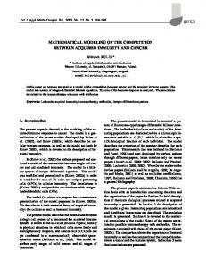
 Distributed vs. Lumped; depending on changing variables in time and space domains.  Linear vs. Nonlinear; depending on the variable power in governing equation.  Analytical vs. Numerical; depending on closed form solution availability. Deterministic models are built of algebraic and differential equations, while probabilistic models include statistical features. In continuous systems, changes occur continuously as time advances evenly, while in discrete models, changes occur only when discrete events occur, irrespective of time passage. In static models, the results are obtained by a single computation of all equations while in dynamic models are obtained by repetitive computation of all equations as time passes. Lumped static models are often built of algebraic equations; lumped dynamic models are often built of ordinary differential equations; and distributed models are often built of partial differential equations. When an equation contains only one variable in each term and each variable appears only to the first power, that equation is termed linear, if not, it is known as nonlinear. Linear models satisfy the principle of super-positioning. When all the equations in a model can be solved algebraically to yield a solution in a closed form, the model can be classified as analytical, if not, a numerical model is required to solve system of equations. These classifications are presented to stress the necessity of understanding input data requirements, model formulation, solution procedures, and to guide in the selection of the appropriate computer software tool in modeling system. Most environmental systems can be approximated in a satisfactory manner by linear and time variant descriptions in a lumped or distributed manner, at least for specified and restricted conditions. Analytical solutions are possible for limited types of systems; while computer based mathematical modeling using numerical solutions provide solutions for problems of complex geometry and properties. Figure (1) shows classification of mathematical models while Table 1 highlights typical uses of mathematical models.

Figure (1): Classification of mathematical models (N=number of variables), (1).

9

Bakenaz A. Zeidan


2015

Table 1: Typical Uses of Mathematical Models (1). Environmental Issues/ concerns media Atmosphere Hazardous air pollutants, air emissions, toxic releases, acid rain; particulates, smog, CFCs, health concerns

Use of models in Concentration profiles; exposure; design and analysis of control processes and equipment; evaluation of management actions; environmental impact assessment of new projects; compliance with regulations Fate and transport of pollutants; concentration plumes; design and analysis of control processes and equipment; waste load allocations; evaluation of management actions; environmental impact assessment of new projects; compliance with regulations Fate and transport of pollutants; design and analysis of remedial actions; drawdowns; compliance with regulations Fate and transport of pollutants; concentration plumes; design and analysis of control processes; evaluation of management actions

Surface water

Wastewater treatment plant discharge; industrial discharges; agricultural/urban runoff; storm water discharge; potable water source; food chain

Groundwater

Leaking underground storage tanks; leachates from landfills and agriculture; injection; potable water source Land application of solid and hazardous wastes; spills; leachates from landfills; contamination of potable aquifers Sludge disposal; spills; Fate and transport of pollutants; outfalls; food chain concentration plumes; design and analysis of control processes; evaluation of management actions

Subsurface

Ocean

4.4.

Environmental Models

Mathematical models in the environmental field can be traced to back to the 1900s, the pioneering work of Streeter and Phelps on dissolved oxygen being the most cited. Today, driven mainly by regulatory forces, environmental studies have to be multidisciplinary, dealing with a wide range of pollutants undergoing complex biotic and abiotic processes in the soil, surface water, groundwater, and atmospheric compartments of the ecosphere. In addition, environmental studies also encompass equally diverse engineered reactors and processes that interact with the natural environment through pathways. Consequently, modeling of large scale environmental systems is often a complex and challenging task. The impetus for developing environmental models can be one or more of the following (1):  To gain better understanding of and glean insight into environmental processes and their influence on the fate and transport of pollutants in the environment.  To determine short and long term chemical concentrations in the various compartments of the ecosphere for use in regularity, enforcement, and in the

10

Bakenaz A. Zeidan


2015

assessment of exposures, impacts, and risks of existing as well as proposed chemicals.  To predict future environmental concentrations of pollutants under various waste loadings and/or management alternatives.  To satisfy regulatory and statutory requirements relating to environmental emissions, discharges, transfers, and releases of controlled pollutants.  To use hypothesis testing relating to processes, pollution control alternatives, etc.  To implement in the design, operation, and optimization of reactors, processes, pollution control alternatives, etc.  To simulate complex systems at real, compressed, or expanded time horizons that may be too dangerous, too expensive, or too elaborate to study under real conditions.  To generate data for post-processing, such as statistical analysis, visualization analysis, and animation, for better understanding, communication, and dissemination of scientific information.  To use environmental impact assessment of proposed new activities that is currently nonexistent. In environmental systems, nonlinearities and spatial and temporal lags prevail. However, all too often these system features are moved to the sidelines of scientific investigations. As a consequence, the presence of nonlinearities and spatial and temporal lags significantly reduces the ability of these investigations to provide insights that are necessary to make proper decisions about the management of complex ecological– economic systems. New modeling approaches are required to effectively identify, collect, and relate the information that is relevant for understanding those systems, to make consensus building an integral part of the modeling process, and to guide management decisions.

4.5.

Natural Models

Modeling of natural environmental systems had lagged behind the modeling of engineered systems. While engineered systems are well defined in space and time; better understood; and easier to monitor, control, and evaluate, the complexities and the uncertainties of natural systems have rendered their modeling a difficult task. However, increasing concerns about human health and degradation of the natural environment by anthropogenic activities and regulatory pressures have driven modeling efforts toward natural systems. Better understanding of the science of environment, experience from engineered systems, and the availability of desktop computing power also contributed to significant inroads into modeling of natural environmental systems. Modeling studies that began with BOD and dissolved oxygen analyses in rivers 1920s have grown to include nutrients and toxicants, lakes to groundwater, sediments to unsaturated zones, waste load allocations to risk analysis, single chemicals to multiphase flow, and local to global scales. Today, environmental models are used to evaluate the impact of past practices, analyze conditions to define suitable remediation or management approaches, and forecast future fate and transport of contaminants in the environment. Modeling of the natural environment is based on the material balance concept. Obviously, a prerequisite for preforming a material balance concept is an understanding of various processes and reactions of that the substance might undergo in

11

Bakenaz A. Zeidan


2015

the natural environment and an ability to quantify them. The material balance approach is the primary principle upon which mathematical models of environmental systems are built. It is based on the principle of conservation of mass ―mass can neither be created nor destroyed”. Material balance is attained through diffusive, advective and dispersive transport processes.

4.6.

Statistical Models

Statistical approaches based on historical or cross sectional data often are used to quantify the relationships among system components. To be able to deal with multiple feedbacks among system components and with spatial and temporal lags requires the availability of rich data sets and elaborate statistical models. Recent advances in statistical methods have significantly improved the ability to test for the goodness of fit of alternative model specifications and have even attempted to test for causality in statistical models. Typically, little attention is given to first principles in attempts to use statistical models to arrive at a better understanding of the cause-effect relationships that lead to system change. Model results are driven by data, the convenience of estimation techniques, and statistical criteria—none of which ensure that the fundamental drivers for system change are satisfactorily identified. By the same token, a statistical modeling exercise can only provide insight into the empirical relationships over a system‘s history or at a point in time, but it is of limited use for analyses of a system‘s future development path under alternative management schemes. In many cases, those alternative management schemes include decisions that have not been chosen in the past, and their effects are therefore not captured in the data of the system‘s history or present state.

4.7.

Dynamic Models

Dynamic modeling is a distinct from of statistical modeling by building into the representation of a phenomenon those aspects of a system that we know actually exist— such as the physical laws of material and energy conservation that describe input–output relationships in industrial and biological processes. Dynamic modeling therefore starts with an advantage over the purely statistical or empirical modeling schema. It does not rely on historic or cross-sectional data to reveal those relationships. This advantage also allows dynamic models to be used in more related applications than empirical models— dynamic models are more transferable to new applications because the fundamental concepts on which they are built are present in many other systems. Computers have come to play a large role in developing dynamic models for decision-making support in complex systems. Their ability to numerically solve for complex nonlinear relationships among system components and to deal with time and space lags and disequilibrium conditions make obsolete the use of linear functional relationships or restriction of the analysis to equilibrium points. It is inappropriate to think of models as anything but crude—yet in many cases absolutely essential—abstract representations of complex interrelationships among system components. Their usefulness can be judged by their ability to help solve decision problems as the dynamics of the real system unfold. They are interactive tools that reflect the processes that determine system change and respond to the choices made by a decision maker.

12

Bakenaz A. Zeidan


2015

5. WHAT IS SIMULATION? A simulation of a system is the operation of a model of the system. The model can be reconfigured and experimented with; usually, this is impossible, too expensive or impractical to do in the system it represents. The operation of the model can be studied, and hence, properties concerning the behavior of the actual system or its subsystem can be inferred. In its broadest sense, simulation is a tool to evaluate the performance of a system, existing or proposed, under different configurations of interest and over long periods of real time. Simulation is used before an existing system is altered or a new system built, to reduce the chances of Figure 2: Simulation Study failure to meet specifications, to eliminate Scheme unforeseen bottlenecks, to prevent under or over-utilization of resources, and to optimize system performance. For instance, simulation can be used to answer questions like: What is the best design for a new telecommunications network? What are the associated resource requirements? How will a telecommunication network perform when the traffic load increases by 50%? How will a new routing algorithm affect its performance? Which network protocol optimizes network performance? What will be the impact of a link failure? The subject of this tutorial is discrete event simulation in which the central assumption is that the system changes instantaneously in response to certain discrete events. For instance, in an M/M/1 queue – a single server queuing process in which time between arrivals and service time are exponential - an arrival causes the system to change instantaneously. On the other hand, continuous simulators, like flight simulators and weather simulators, attempt to quantify the changes in a system continuously over time in response to controls. Discrete event simulation is less detailed (coarser in its smallest time unit) than continuous simulation but it is much simpler to implement, and hence, is used in a wide variety of situations. Figure 2 is a schematic of a simulation study. The iterative nature of the process is indicated by the system under study becoming the altered system which then becomes the system under study and the cycle repeats. In a simulation study, human decision making is required at all stages, namely, model development, experiment design, output analysis, conclusion formulation, and making decisions to alter the system under study. The only stage where human intervention is not required is the running of the simulations, which most simulation software packages perform efficiently. The important point is that powerful simulation software is merely a hygiene factor - its absence can hurt a simulation study but its presence will not ensure success. Experienced problem formulators and simulation modelers and analysts are indispensable for a successful simulation study. The steps involved in developing a simulation model, designing a simulation experiment, and performing simulation analysis are, Figure 3:

13

Bakenaz A. Zeidan


2015

Step 1. Identify the problem. Step 2. Formulate the problem. Step 3. Collect and process real system data. Step 4. Formulate and develop a model. Step 5. Validate the model. Step 6. Document model for future use. Step 7. Select appropriate experimental design. Step 8. Establish experimental conditions for runs. Step 9. Perform simulation runs. Step 10. Interpret and present results. Step 11. Recommend further course of action. Although this is a logical ordering of steps in a simulation study, much iteration at various sub-stages may be required before the objectives of a simulation study are achieved. Not all the steps may be possible and/or required. On the other hand, additional steps may have to be performed.

Figure 3: Modeling process flow chart

6. Environmental Problems Effective management and planning of resources and environmental systems have been of concerns in the past decades since contamination and resource-scarcity problems

14

Bakenaz A. Zeidan


2015

have led to a variety of impacts and liabilities. However, achieving a reasonable and efficient management strategy is difficult since many conflicting factors have to be balanced due to complexities of the real-world problems. In resources and environmental systems, there are a number of factors that need to be considered by planners and decision-makers, such as social, economic, technical, legislation, institutional, and political issues, as well as environmental protection and resources conservation. Moreover, a variety of processes and activities are interrelated to each other, resulting in complicated systems with interactive, dynamic, nonlinear, multi-objective, multistage, multilayer, and uncertain features. These complexities may be further amplified due to their association with economic consequences if the promises of expected targets are violated. Mathematical models are recognized as effective tools that could help examine economic, environmental, and ecological impacts of alternative pollution-control and resources-conservation actions, and thus aid planners or decision-makers in formulating cost-effective management policies. Therefore, to facilitate more robust management and planning of resources and environmental systems, innovative mathematical tools that are able to reflect various combinations of these complexities are desired. This special issue is devoted to provide a forum for facilitating discussions of emerging technologies for supporting decisions of resources and environmental management. It focuses on exposition of innovative methodologies for tackling challenges in modeling a variety of resources and environmental problems, as well as successful case studies. A number of state-of-the-art mathematical modeling studies related to resources and environmental systems are presented, which can help analyze the relevant information, simulate the related processes, implement pollutant mitigations, evaluate the resulting impacts, and generate sound decision alternatives. We begin this introduction to mathematical modeling of environmental problems with an explanation of basic concepts and ideas, which includes definitions of terms such as system, model, simulation, mathematical model, reflections on the objectives of mathematical modeling and simulation, on characteristics of ‗‗good‘‘ mathematical models, and a classification of mathematical models. Any professional in this field, however, should of course know about the principles of mathematical modeling and simulation. Our starting point is the complexity of the problems treated in science and engineering. Difficulty of problems treated in science and engineering typically originates from the complexity of the systems under consideration, and models provide an adequate tool to break up this complexity and make a problem tractable. After giving general definitions of the terms system, model, and simulation, we move on toward mathematical models, where it is explained that mathematics is the natural modeling language in science and engineering. The relatively recent increase in computational power available for mathematical modeling and simulation raises the possibility that modern numerical methods can play a significant role in the analysis of complex environmental problems. The analysis of systems of applied sciences, e.g. technology, economy, biology etc., needs a constantly growing use of methods of mathematics and computer sciences. In fact, once a physical

15

Bakenaz A. Zeidan


2015

system has been observed and phenomenological analyzed, it is often useful to use mathematical models suitable to describe its evolution in time and space. Indeed, the interpretation of systems and phenomena, which occasionally show complex features, is generally developed on the basis of methods which organize their interpretation toward simulation. When simulations related to the behavior of the real system are available and reliable, it may be possible, in most cases, to reduce time devoted to observation and experiments. Bearing in mind the above reasoning, one can state that there exists a strong link between applied sciences and mathematics represented by mathematical models designed and applied, with the aid of computer sciences and devices, to the simulation of systems of real world.

7. Fundamentals of Environmental Processes Contaminants can be transported through a system by microscopic and macroscopic mechanisms such as diffusion, dispersion and advection. At the same time, they may or may not undergo a variety of physical, chemical, and biological processes within the system. Some of these processes result in changes in the molecular nature of the contaminants, while others result in mere change of phase or separation. The former type of processes can be categorized as reactive processes and the latter as nonreactive processes. Those contaminants that do not undergo any significant processes are called conservative substances, and those that do are called reactive substances. A clear mechanistic understanding of the processes that impact the fate and transport of contaminants is a prerequisite in formulating the mathematical model.

7.1. Material Content Material content is a measure of the material contained in a bulk medium, quantified by the ratio of the amount of material present to the amount of the medium. The amount can be expressed in terms of mass, moles, or volume. Material content in liquid phases is often quantified as mass concentration molar concentration or mole fraction. The material content in solid phases is often quantified by ratio of masses and is expressed as ppm or ppb. The material in gas phases is often quantified by a ratio of moles or volumes and is expressed as ppm or ppb. It is important to specify the pressure and temperature in this case.

7.2. Phase Equilibrium Suppose a mass, m, of a chemical is injected into a closed air-water binary system, this system is allowed to reach equilibrium. Under that condition, some of the chemical would have partitioned into the aqueous phase and the balance into the gas phase, assuming negligible adsorption onto the walls of the containers. The chemical content in the aqueous and gas phases are now measured (as mole fractions). For most chemicals, when the aqueous phase content is dilute, a linear relationship could be observed between the phase content. This phenomenon is referred to as linear partitioning. Such linearity has been observed for most chemicals in many two-phase environmental systems. Several fundamental laws from physical chemistry and thermodynamics can be applied to environmental systems under certain conditions. These laws serve as important links between the state of the system, chemical properties, and their behavior. Ideal Gas Law, Dalton‘s Law, Raoult‘s Law, and Henry Law are typical laws of equilibrium (1).

7.3. Environmental Transport Processes Chemicals can be transported through the various compartments of the environment by microscopic level and macroscopic level processes. At the microscopic level, the primary mechanism of transport is by molecular diffusion driven by concentration gradients. At the macroscopic level, mixing and bulk movement of the medium are the primary transport

16

Bakenaz A. Zeidan


2015

mechanisms. Transport by molecular diffusion and mixing has been referred to as dispersive transport, while transport by bulk movement of the medium is referred to as advective transport. Advective and dispersive transport is fluid-element driven, whereas diffusive transport is concentration-driven and can be proceed under quiescent conditions.

7.4. Interphase Mass Transport The transfer of mass from one phase to another is an important transport process in environmental systems. Examples of such processes include aeration, re-aeration, air stripping, soil emissions, etc. The following theories have been proposed to model such transfers: the TwoFilm Theory proposed in 1920s, the Penetration Theory proposed in the 1930s, and the Surface Renewal Theory proposed in 1950s. Among these, the first is the simplest, most understood, and most commonly used (1).

7.5.

Environmental Nonreactive Processes

Nonreactive processes cause changes in the chemical content within the system, without the chemical undergoing any changes in its molecular structure; the chemical may undergo a phase change. Such processes are referred to as physical processes. Some examples of environmental nonreactive processes are settling, re-suspension, floatation, adsorption, desorption, absorption, thermal desorption, volatilization, extraction, filtration, membrane processes, and bio sorption.

7.6. Environmental Reactive Processes Reactive processes result in changes in concentrations of chemicals within a system by degrading or transforming them to different chemicals. Reactions can occur in a single step (elementary reactions) or in multiple steps, consecutively, in parallel, or in cycles. Some of the most common environmental reactive processes are biodegradation, hydrolysis, oxidation, reduction, incineration, precipitation, ion exchange, and photolysis. Reactive processes can be categorized as homogeneous if they occur only in a single phase or heterogeneous if they involve multiple phases.

7.7. Material Balance The material balance approach is the primary principle upon which mathematical models of environmental systems are built. It is based on the principle of conservation of mass ―mass can neither be created nor destroyed” Before applying the material balance principle, the following preliminaries have to be addressed:  Define and characterize the system and the boundary  Identify the inflows and outflows of the target chemical crossing the boundary  Identify all sources and sinks of the target chemical inside the system  Identify all reactive and nonreactive processes acting upon the target chemical. In the verbal form, the material balance equation can be stated as follows: Net rate of change of = Rate of inflow of - Rate of outflow of ± Rate of reactions material within material into system + material from system within system system The material balance equation can be applied for distributed systems and lumped systems.

17

Bakenaz A. Zeidan


2015

8. Steps in Developing Mathematical Models The craft of mathematical model development is part science and part art. It is a multistep, iterative, trial-and-error process cycling through hypotheses formation, inference, testing, validating, and refining. While the scientific side of modeling involves the integration of knowledge to build the model, the artistic side involves the making of a sensible compromise and creating balance between two conflicting features of the model: degree of detail, complexity, and realism on hand, and the validity and utility value of the final model on the other.

8.1. Problem formulation Formulation of the problem is the first step in the mathematical model development process. This step involves the following tasks: 1- Establishing the goal of the modeling effort. 2- Characterizing the system 3- Simplifying and idealizing the system

Approach to mathematical modeling Problem Formulation Mathemtical Representation Mathematical analysis Interpretation and Evaluation of Results Figure 4: Overall approach to mathematical modeling

8.2. Mathematical presentation The most crucial step in the process, requiring in-depth subject matter expertise. This step involves the following tasks: 1. Identifying fundamental theories. 2. Deriving relationships 3. Standardizing relationships

8.3. Mathematical analysis The next step of analysis involves application of standard mathematical techniques and procedures to ―solve‖ the model to obtain the desired results. The analysis is done according to the rules of mathematics and the system has nothing to do with the process.

18

Bakenaz A. Zeidan


2015

8.4. Interpretation and evaluation of results It is during this step that the iteration and model refinement process is carried out. During the iterative process, performance of the model is compared against the real system to ensure that the objectives are satisfactorily met. This process consists of two main tasks; calibration and validation. 1. Task 1: Calibrating the model; in the calibration process, previously observed data from the real system are used as a ―training‖ set. The model runs repeatedly, adjusting the model parameters by trial and error until its predictions under similar conditions match the training data set as per his goals and performance criteria. An efficient way to calibrate a model is to perform preliminary sensitivity analysis on model outputs to each parameter one by one. If the model cannot be calibrated to be within acceptable limits, the modeler should backtrack and reevaluate the system characterization and/or the model formulation steps. This iterative exercise is critical in establishing the utility value of the model and the validity of its applications, such as making predictions for the future. 2. Task 2: Validating the model: A model can be considered valid if the agreement between the two under various conditions meets the goal and performance criteria. A common practice used to demonstrate validity is to generate a parity plot of predicted vs. observed data with associated statistics such as goodness of fit. Another method is to compare the plots of predicted values and observed data as a function of distance or time and analyze the deviations.

Figure 5: Model Calibration

Summing up, empirical models are used to fill in where scientific theories are nonexistent or too complex. Experimental or physical model results are used to develop empirical models and calibrate and validate mathematical models. Figure c illustrates a flow chart for steps of a developing a mathematical model.

9. SQM SPACE OF MATHEMATICAL MODELS To understand mathematical models, let us start with a general definition. Many different definitions of mathematical models can be found in the literature. The differences between these definitions can usually be explained by the different scientific interests of their authors. For example, many economical or sociological problems cannot

19

Bakenaz A. Zeidan


2015

be treated in a time-space framework or based on equations only. A mathematical model (S, Q, and M) is called in stationary, if at least one of its system parameters or state variables depends on time and stationary otherwise. A mathematical model (S, Q, and M) is called distributed, if at least one of its system parameters or state variables depends on a space variable, lumped otherwise. A critical element of model-based decision support is a mathematical model, which represents data and relations that are too complex to be adequately analyzed based solely on experience and/or intuition of a DM or his/her advisors. Models, when properly developed and maintained, can represent not only a part of knowledge of a DM but also integrate relevant knowledge available from various disciplines and sources. Moreover, models, if properly analyzed, can help the DM to extend his/her knowledge and intuition. However, models can also mislead users by providing wrong or inadequate information. Such misinformation can result not only from flaws or mistakes in model specification and/or implementation, the data used, or unreliable elements of software, but also by misunderstandings between model users and developers about underlying assumptions, limitations of applied methods of model analysis, and differences in interpretation of results, to name a few. Therefore, the quality of the entire modeling cycle determines to a large extent the quality of the decision-making process for any complex decision problem, (Makowski, 2001).

Based on the examples in the last section, the reader can now distinguish between some basic classes of mathematical models. We will now widen our perspective toward a look at the entire ‗‗space of mathematical models‘‘, that is, this section will give you an idea of various types of mathematical models that are used in practice. The practical use of a classification of mathematical models lies in the fact that you understand ‗‗where you are‘‘ in the space of mathematical models, and which types of models might be applicable to your problem beyond the models that you have already used. The ‗‗space of mathematical models‘‘ evolves naturally a mathematical model to be a triple (S, Q, M) consisting of a system S, a question Q, and a set of mathematical statements M. Based on this definition, it is natural to classify mathematical models in an SQM space. Figure 6a shows one possible approach to visualize this SQM space of mathematical models, based on a classification of mathematical models between black and white box models. Psychological and social systems constitute the ‗‗black box‘‘ end of the spectrum. Only very vague phenomenological models can be developed for these systems due to their complexity and due to the fact that too many sub-processes are involved which are not sufficiently understood. On the other hand, mechanical systems, electrical circuits etc. are at the white box end of the spectrum since they can be very well understood in terms of mechanistic models (a famous example is Newton‘s model of planetary motion). Note that the three dimensions of a mathematical model (S, Q, M) can be seen in the figure: the systems (S) are classified on top of the bar, immediately below the bar there is a list of objectives that mathematical models in each of the segments may have (which is Q), and at the bottom end there are corresponding mathematical structures (M) ranging from algebraic equations (AEs) to differential equations (DEs). As suggested by Figure 6, black box regression models of this kind are widely used for the modeling for example, of psychological, social, or economic systems.

20

Bakenaz A. Zeidan


2015

Figure 6: SQM Space of Mathematical Models The ‗‗Q‘‘-criteria in Figure 6a illustrate that mathematical models can be used. To solve increasingly challenging problems as the model gradually turns from a black box to a white box model. At the black box end of the spectrum, models can be used to make more or less reliable predictions based on data. At the white box end of the spectrum, mathematical models can be applied to design, test, and optimize systems and processes on the computer before they are actually physically realized. This is used e.g. in virtual engineering, which includes techniques such as interactive design using CFD or virtual prototyping. As an example, you may think of the computation of the temperature distribution within a three-dimensional device using finite-element software. Based on the method described there, what-if studies can be performed, that is, it can be investigated what happens with the temperature distribution if you change certain characteristics of the device virtually on the computer, and this can then be used to optimize the construction of the device so as to achieve certain desired characteristics of the temperature distribution.

9.1.

SQM Space Classification: S Axis

Since mathematical models are characterized by their respective individual S, Q and M ‗‗values‘‘, one can also think of each model as being located somewhere in the ‗‗SQM space‘‘ of Figure 6b. On each of the S-, Q- and M-axes of the figure, mathematical models are classified with respect to a number of criteria which were compiled based on various classification attempts in the literature. Let us explain these criteria, beginning with the S axis of Figure 6b: Physical – conceptual. Physical systems are part of the real world, for example, a fish or a car. Conceptual systems are made up of thoughts and ideas, for example, a set of mathematical axioms. This book focuses entirely on physical systems. Natural – technical. Naturally, a natural system is a part of nature, such as a fish or a flower, while a technical system is a car, a machine, and so on. An example of a natural system is the predator–prey system and the stormier viscometer exemplifies a technical system. Stochastic – deterministic. Stochastic systems involve random effects, such as rolling dice, share prices and so on. Deterministic systems involve no or very little random effects, for example, mechanical systems, such as the planetary system, a pendulum, and

21

Bakenaz A. Zeidan


2015

so on. In a deterministic system, a particular state A of the system is always followed by one and the same state B, while A may be followed by B, C or other states in an unpredictable way if the system is stochastic. Continuous – discrete. Continuous systems involve quantities that change continuously With time, such as sugar and ethanol concentrations in a wine fermenter. Discrete systems, on the other hand, involve quantities that change at discrete times only, such as the number of individuals in animal populations. Note that on the M axis of Figure 6, continuous systems can be represented by discrete mathematical statements and vice versa. Dimension. Depending on their spatial symmetries, physical systems can be described using 1, 2, or 3 space variables. The number of space variables used to describe a physical system is called its dimension (frequently denoted 1D, 2D, or 3D). Examples: a 1D river simulation and a 3D temperature distribution. Field of application. We can distinguish between chemical systems, physical systems, biological systems, and so on.

9.2. SQM Space Classification: Q Axis On the Q- axis of Figure 6b, we have the following categories: Phenomenological – mechanistic and Stationary – in stationary. It depends on the question which we are asking (i.e. on the ‗‗Q‘‘ of a mathematical model (S, Q, M)) whether a stationary (time-independent) or instationary (time-dependent) model is appropriate. Lumped – distributed. It depends on the question which we are asking (i.e. on the ‗‗Q‘‘ of a mathematical model (S, Q, M)) whether a lumped (space-independent) or distributed (space-dependent) model is appropriate. The wine fermentation model is an example of a lumped model since it does not use spatial coordinates. On the other hand, the computation of a 3D temperature distribution is based on a distributed model. Direct – inverse. If Q assumes given input and system parameters and asks for the output, the model solves a so-called direct problem. Most of the models below refer to direct problems. If, on the other hand, Q asks for the input or for parameters of S, the model solves a so-called inverse problem. If Q asks for parameters of S, the resulting problem is also called a parameter identification problem. Examples are the regression and neural network models, and the fitting of ODEs to data. If Q asks for input parameters, the resulting problem is also called a control problem, since in this case the problem is to control the input in a way that generates some desired output. Research – management. Research models are used if Q aims at the understanding of S; management models, on the other hand, are used if the focus is on the solution of practical problems related to S. Research models tend to be more complex and less manageable from a practical point of view. Depending on Q, the same mathematical equations can be a part of a research or of a management model. Speculation – design - Scale. Depending on Q, the model will describe the system on an appropriate scale. For example, depending on Q it can be appropriate to virtually follow a fluid particle on its way through the complex channels of a porous medium, or just to compute the pressure drop across a porous medium based on its permeability. Obviously, these cases correspond to a description of a porous medium on two scales microscopic/macroscopic.

22

Bakenaz A. Zeidan


2015

9.3. SQM Space Classification: M Axis Linear – nonlinear. In linear models, the unknowns (or their derivatives) are combined using linear mathematical operations only, such as addition/subtraction or multiplication with parameters. Nonlinear models, on the other hand, may involve the multiplication of unknowns, the application of transcendental functions, and so on. Nonlinear models typically have more (and more interesting) solutions but are harder to solve. Examples are linear or nonlinear regression models. Analytical – numerical. In analytic models, the system behavior can be expressed in terms of mathematical formulas involving the system parameters. Based on these models, qualitative effects of parameters and the entire system behavior can be studied theoretically, without using concrete values for the parameters. Numerical models, on the other hand, can be used to obtain the system behavior for specific parameter values. Autonomous – no autonomous. This is a mathematical classification of in stationary models. If an equation does not depend explicitly on time, it is called autonomous, otherwise nonautonomous. Continuous – discrete. In continuous models, the independent variables may assume arbitrary (typically real) values within some interval. In discrete models, on the other hand, the independent variables may assume some discrete values only. Difference equations. In difference equations, the quantity of interest is obtained as a sequence of discrete values. Usually, this is expressed in terms of recurrence relations in which each term of the sequence depends on previous terms. Difference equations are frequently used to describe discrete systems. Differential equations. Differential equations are equations involving derivatives of an unknown function. They are a main tool to set up continuous mechanistic models. Integral equations. Integral equations are equations involving an integral of an unknown function. Algebraic equations. AEs are equations involving the usual algebraic operations such as addition, subtraction, division, and so on. Note that some of the above categorizations of mathematical models overlap. For example, both phenomenological and mechanistic models can be lumped or distributed, stationary or instationary, and so on. Thus, it may have confused the reader if a single chapter would have been devoted to each of these categorizations. The other categorizations are treated within this perspective, that is, they will be referred to in the context of appropriate examples. Note that referring to Figure 1.11b we can say that the categorization of mathematical models between phenomenological and mechanistic models divides the SQM space of mathematical models into two different ‗‗half-spaces‘‘ along the Q-axis. You understand the message: People always tend to solve problems similar to the way in which they successfully solved problems in the past. Yesterday, our problem might have been to drive a nail into a piece of wood, and we might have solved this problem adequately using a hammer. Today, however, we may have to drive a screw into a piece of wood, and it is of course not quite such a good idea to use the hammer again. Similarly, mathematical models are like tools that help us to solve problems, and we will always tend to reuse the models that helped us to solve our yesterday‘s problems. This is like a law of nature in mathematical modeling, similar to Newton‘s law of inertia; let us call it the ‗‗law of inertia of mathematical modeling‘‘. Forces need to be applied to physical bodies to change their state of motion, and

23

Bakenaz A. Zeidan


2015

in a similar way forces need to be applied in a mathematical modeler‘s mind before he will eventually agree to replace established models by more adequate approaches. Even great scientists such as A. Einstein were affected by this kind of inertia. Einstein did not like the idea that the physical universe is probabilistic rather than deterministic. 10.

Groundwater Flow and Solute Transport Modeling

Those that are new to groundwater modeling are often overwhelmed with terms such as finite differences, finite elements, grid discretization and triangulation. Once you gain a basic understanding of the terms and the processes involved in groundwater modeling, you are often faced with the ultimate question "Which numerical method should I use for my project?" The answer is not often so much what you should use but often is based on what method or software package is readily available. Like most people, groundwater modelers want to stick with what they know. There are, however, two main numerical methods that should be considered: Finite Difference Method and Finite Element Method.

10.1. Governing Equations General governing equation for groundwater flow for three dimensional unconfined, transient, heterogeneous, and anisotropic groundwater flow reads:

 h  h  h h ( Kx )  ( Ky )  ( Kz )  Ss  R * x x y y z z t where: Kx, Ky, Kz: hydraulic conductivity tensor; h: hydraulic head; Ss: storage coefficient; R: source or sink Bear (1987) presented the basic equations of contaminant transport in groundwater. He presented two component for hydrodynamic dispersion of the contaminant concentration; advective transport and dispersive transport. Dispersive flux is a macroscopic flux that expresses the effect of the microscopic variation of the velocity.

=

(

)-

(

)+

+∑

where: Dissolved concentration of species k, ML-3; n porosity of the subsurface medium, dimensionless; t time, T; xi distance along the respective Cartesian coordinate axis, L; Hydrodynamic dispersion coefficient tensor, L2T-1; Seepage or linear pore water velocity; LT-1; it is related to the specific discharge or Darcy flux through the relationship, vsi=qi/n; volumetric flow rate per unit volume of aquifer representing fluid sources (positive) and sinks (negative), T-1;

24

Bakenaz A. Zeidan


2015

Concentration of the source or sink flux for species k, ML-3; Chemical reaction term, ML-3T-1. Dispersion in porous media refers to the spreading of contaminants over a greater region than would be predicted solely from the average groundwater velocity vectors.

10.2. Finite Difference Model

Figure 7: Finite Difference Mesh MODFLOW uses the finite differences method to solve the groundwater flow equation. The grid is created using structured, rectilinear (rectangular) grids. This method is widely used and accepted by many governing bodies. It is the most popular groundwater simulator available, is open source and is well documented. The finite difference solution is easy to understand and calculate, the solutions are massconservative and there are several numerical extensions available such as PEST, transport, particle tracking and zone budget. However, the finite difference method is not without weakness. Although grids are easy to create, they cannot be efficiently refined around areas of interest, such as wells and model boundaries. This can be partially addressed by the MODFLOW-LGR (Local Grid Refinement) extension. Complex geology is difficult to represent particularly if there are discontinuous or pinched out layers; when there are steep gradients in the stratigraphy, this can result in disconnected cells which causes problems with running the model. MODFLOW requires model layers to be continuous across the entire model domain, making it a challenge to model smaller formations of materials (lenses) within a larger body, without adding a large number of unnecessary cells. MODFLOW provides an approximate representation of variable anisotropy in model parameters (e.g. it only uses the principle components of the hydraulic conductivity tensor; Kxx, Kyy and Kzz), and therefore is limited for modeling faults and fractures.

25

Bakenaz A. Zeidan


2015

10.3. Finite Element Model

Figure 8: Finite Element Mesh The finite element method can also be used to solve the groundwater flow equation. There are several codes available; FEFLOW being the most popular. FEFLOW uses a finite element (triangular) mesh to represent the model domain. The use of triangles allows for a more efficient refinement around wells and boundaries. The triangular mesh can more easily adapt to variable stratigraphy such as sloping or pinch outs, and allows for versatile discretization of non-rectangular model domains. Finite element methods provide a better representation of anisotropy (fully represents conductivity tensor – each triangular element is given its own coordinate system, whereas MODFLOW requires conductivity to be perpendicular to the faces of the finite difference cells (horizontally rectangular)). No method is perfect; with finite elements the local mass conservation is not guaranteed. There can be discontinuous velocities at the element boundaries which can make it difficult to determine unique path lines. FEFLOW is similar to MODFLOW in that model layers must be continuous across the entire model domain. In order to represent smaller formations within larger bodies, an entire model layer must be inserted with a minimum layer thickness enforced in the discontinuous regions.

26

Bakenaz A. Zeidan


2015

Figure 9: Finite Element Mesh

11.

Modeling System for Landform and Urban Area

A number of natural disasters occur annually in various parts of the world. Especially, a number of natural disasters in cities increases in accordance with the development of city area, such as flood, wind disaster and air pollution. In order to estimate the extent of a disaster quantitatively, it is necessary to estimate the behavior of natural phenomena which causes the natural disaster. In practical computations of this type of problems, the computational domain is large and the computations need to be carried out over long time durations. Therefore, this type of problem becomes quite largescale and it is essential to use methods which are as efficient and fast as the available hardware allows. In recent years, massively parallel finite element computations have been successfully applied to several large-scale simulations for natural phenomena. These computations demonstrated the availability of a new level of computational capability to solve practical problems. However, in order to compute natural phenomena accurately, it is necessary to prepare an accurate shape model for landform, buildings and civil structures. Furthermore, a good finite element mesh of quality must be prepared for the complicated spatial analytical domain. In the present study, a large-scale computer modeling and simulation method is presented for environmental flows in urban area. Several GIS and CAD data were used for the preparation of shape model and an automatic mesh generation method based on Delaunay method was developed. In order to express the geographical features accurately, the valley and ridge lines are expressed by an edge of the element. ArcView and AutoCAD are employed for the GIS and CAD systems respectively. Parallel finite element method based on domain decomposition method and MPI was employed for the numerical simulation of natural phenomena. The P1/P1 element (triangular element for 2D problem, tetrahedral element for 3D problem) was employed for the finite element. The stabilized finite element formulation based on SUPG/PSPG was employed for the discretization in space. The present method was applied to the simulation of flood flow and wind flow in urban area. The shallow water equation and the Navier-Stokes equation

27

Bakenaz A. Zeidan


2015

were employed for the governing equations. The present method is shown to be a useful planning and design tool for natural disasters and the change of environments.

Figure 10: Flow chart for the modeling system for landform

11.1. Modeling for Landform Figure 10 shows the flow chart for the modeling system for landform. For the data of land elevation, the digital elevation map issued by the Japanese geographical survey institute was employed. The resolution of the map is 50m. The ArcView was used for the GIS system. Using the data of elevation map, a finer grid was created by third order spline interpolation method. The grid is referred as the grid surface and the grid size was assumed to be 10m. Figure 11 shows the grid surface and contour line for the studied area. The information of valley and ridge line is created by the function of ArcView using the elevation data of grid surface. Figure 12 shows the contour-, valley and ridge lines.

28

Bakenaz A. Zeidan


Figure 11 Grid surface and contour line for studied area

2015

Figure 12: Contour line, valley and ridge lines

Next, the line data was vectored by the raster-vector transformation. The nodes are generated on the contour, valley and ridge lines at the regular interval. The elevation of nodes on the valley and ridge lines are obtained by superposing the elevation data of grid surface. Figure 4 shows the node distribution at the local part of the studied area. ach nodes have the data for plane coordinate and elevation, and the property for line type.

11.2. Modeling for Urban Area The modeling system for urban area is expressed in this section. In case of the modeling of urban area, the building data is needed in addition with the elevation data. For the data for buildings, the 2D and 3D GIS data obtained by the aerial-photo and -laser surveying were employed.

11.2.1.

2D modeling for urban area

The 2D finite element model for flood flow analysis was prepared. For the data for buildings, the 2D GIS data (Mapple 2500) obtained by the aerial-photo was employed. For the data of land elevation, the digital elevation map issued by the Japanese geographical survey institute was employed. Figure 13 shows the contour line and the polygon for buildings after the superposition of both digital elevation map and 2D GIS data for buildings. In case of the modeling of urban area, the nodes are generated on not only the contour line, valley and ridge lines but also the boundary of the building as shown in Figure 14. In this example, the valley and ridge lines are not considered as break lines. Figure 15 shows the finite element mesh for the studied area. The mesh size was assumed to be 2m. Figure 16 shows the details for the finite element idealization around the river.

29

Bakenaz A. Zeidan


Figure 13 Contour line and polygon for buildings line and boundary of building

Figure 15: Finite element mesh

11.2.2.

2015

Figure 14 Nodes on contour

Figure 16: Finite element mesh around river

3D modeling for urban area using 2D GIS data

The 3D finite element model for wind flow analysis was prepared by using the 2D GIS data (Mapple 2500). For the data of land elevation, the digital elevation map issued by the Japanese geographical survey institute was employed. Figure 15 shows the surface mesh around Shinjuku-area, Tokyo. The vertical shape for low-storied buildings was assumed to be straight and that for the high-storied buildings were prepared by the CAD system (Auto CAD). In Figure 16, the color buildings indicate the buildings prepared by the CAD system.

30

Bakenaz A. Zeidan


2015

Figure 17 Shape modeling using CAD system

11.2.3.

3D modeling for urban area using 3D GIS data

The 3D finite element model for wind flow analysis was prepared by using the 3D GIS data (Map Cube). For the major cities, the 3D GIS data was prepared in Japan. Figure 17 shows the 3D GIS data around Ebisu, Tokyo. The 3D GIS data was obtained by the laser surveying. This data contains the surface data for not only the housing and buildings but also the landform accurately. However, data concerning public facilities such as expressways are not available. So, the public facilities are added by using CAD system. Figure 18 shows the 3D shape model after adding the expressway.

Figure 18: 3D GIS data for Ebisu, Tokyo

31

Bakenaz A. Zeidan


2015

11.2.4. Finite Element Simulations The stabilized finite element method was employed for the simulation of environmental flows in urban area. The finite element mesh obtained by the present method were applied to the simulation of flood flow and wind flow in urban area.

11.3. Flood Flow Simulations For the flood flow simulation, the shallow water equation was employed for the governing equations. The stabilized finite element formulation based on SUPG was employed for the discretization in space. For the discretization in time, the explicit Euler method was employed. In order to treat the moving boundary, the Eulerian approach was applied. The finite element mesh shown in Figure 19 was employed for the simulation. The total number of elements and nodes are 33,223 and 53,272 respectively. For the boundary condition, the discharge was assumed at the inlet of river. Figure 19 shows the computed water elevation at t=3 hours. It can be seen that the flood occur in accordance with the increase of river discharge.

Figure 19: Flood flow simulation

11.4. Wind Flow Simulation For the wind flow simulation, the Navier-Stokes equation was employed for the governing equations. The finite element mesh based on the tetrahedral element was prepared by using the 3D shape model shown in Figure 20. The total number of nodes and elements were 2,868,335 and 15,871,126 respectively. The stabilized finite element method based on SUPG/PSPG was employed for the discretization in space, and the Crank-Nicolson scheme was employed for the discretization in time. The parallel computational method based on domain decomposition and MPI was employed. Figure 21 shows the domain decomposition for 20 sub-domains. The PC cluster used consists of 20 nodes, each with an Intel-Xeon 3.06 GHz processors and 2GB memory.

32

Bakenaz A. Zeidan


2015

Figure 21: Domain decomposition

Figure 22 Computed streamline

Summing up, a large-scale computer modeling and simulation method for environmental flows in urban area has been presented in this paper. The shape model for landform and buildings can be prepared accurately by using several GIS and CAD data.

33

Bakenaz A. Zeidan


2015

The automatic mesh generation method based on Delaunay method has been developed. Parallel finite element method based on domain decomposition method has been employed for large scale simulations. The present method has been applied to the simulation of flood flow and wind flow in urban area. From the results obtained in this paper it can be concluded that the present method provides a useful planning and design tool for the natural disasters and the change of environments, (Kashiyama et. al. 1998).

12.

Conclusions

This chapter has a dual objective: first, to introduce the reader to some of the most important and widespread environmental issues of the day; and second, to illustrate the vital role played by mathematical models in investigating these issues. The environmental issues addressed include: ground-water contamination, air pollution, and hazardous material emergencies. These issues are presented in their full real-world context, not as scientific or mathematical abstractions; and for background readers are invited to investigate their presence in their own communities. This chapter of the book leads the reader through relatively elementary modeling of these phenomena, including simple algebraic equations for ground water, slightly more complex algebraic equations (preferably implemented on a spreadsheet or other computerized framework) for air pollution, and a fully computerized modeling package for hazardous materials incident analysis. The interplay between physical intuition and mathematical analysis is emphasized. In summary, the effective mathematical models for managing resources and environmental systems are becoming one of the most important goals pursued by governments, industries, communities, and researchers. These present chapter formulated a variety of mathematical models for supporting natural resources allocation, flooding prevention and control, environmental pollution control, ecological protection, and sustainable development improving, where a number of innovative perspectives and findings are advanced. These mathematical models can (i) describe complex environmental processes and interactions, characterize the spatial and temporal variations, and predict the fate and transport of the contaminants; (ii) assess potential risks existing in various resources-related activists and the associated socioeconomic and environmental impacts under a variety of system conditions; (iii) generate sound decision alternatives for generating desired policies that target on more effective resources and environmental management. This special issue reports the latest research results in mathematical modeling for resources and environmental systems.

References 1. N. Nirmalakahandan (2002) “Modeling Tools for Environmental Engineers and Scientists”, CRC Press LLC 2. Kai Velten (2009),” Mathematical Modeling and Simulation” WILEY-VCH Verlag GmbH & Co. KGaA, Weinheim 2009. 3. Robert J. LABEUR (2009),” Finite element modeling of transport and non-hydrostatic flow in environmental fluid mechanics” PhD. Thesis submitted to Civil Engineering And Geosciences Faculty, Delft University of Technology. 2009 R.J. Labeur, ISBN 97890-8559-528-1

34

Bakenaz A. Zeidan


2015

4. S. Ion, G. Marinoschi and C.Popa (2005)“Mathematical Modeling of Environmental and Life Sciences Problems” Proceedings of the fourth workshop September, 2005, Constanta, Romania 5. B. Jha (2005) “A Mixed Finite Element Framework For Modeling Coupled Fluid Flow and Reservoir Geomechanics”, MSc. in Petroleum Engineering. Submitted to Stanford University 6. R. Costanza And M. Ruth (1998) “Using Dynamic Modeling to Scope Environmental Problems and Build Consensus”, Environmental Management Vol. 22, No. 2, pp. 183– 195. 7. Marek Makowski (2001) “Chapter 3: Modeling Techniques for Complex Environmental Problems” Natural Environment Management and Applied Systems Analysis, M. Makowski and H. Nakayama (Eds.), 2001, International Institute for Applied Systems Analysis, Laxenburg, Austria, ISBN 3-7045-0140-9. 8. K. Kashiyama, H. Hamada, T. Taniguchi, (1998) “Large Scale Finite Element Simulation and Modeling Using GIS/CAD for Environmental Flows in Urban Area” Environmental Management Vol. 22, No. 2, pp. 183–195. 9. Jȍrg Fliege (2008),” Protection of the Environment: Pollution Spread .Mathematical Models and Optimization“(Africa), Regional Sustainable Development Review- Vol. I. 10. Sam O. Ale (2004)” Mathematical Modeling - A Tool For Solving Environmental Problems” Workshop, 2004, National Mathematical Centre Abuja, Nigeria. 11. John W. Boland, Jerzy A. Filar, and Phil G. Howlett (2010) “Environmental Problems, Uncertainty, and Mathematical Modeling”, Notices of the AMS. Volume 57, Number 10. 12. Anu Maria, (1997) “Introduction To Modeling and Simulation” Proceedings of the 1997 Winter Simulation Conference ed. S. Andradóttir, K. J. Healy, D. H. Withers, and B. L. Nelson. 13. https://www.swstechnology.com/blog/groundwater-modeling-numerical-methodswhich-one-should-you-use

35

Bakenaz A. Zeidan

Mathematical Modeling of Environmental Problems

Mathematical Modeling of Environmental Problems

Suggest Documents

Environmental problems indicator under environmental modeling ...

Editorial Nonlinear Problems: Mathematical Modeling ... - Hindawi

MATHEMATICAL MODELING MATHEMATICAL MODELING OF THE

Modeling Techniques for Complex Environmental Problems - CiteSeerX

Survey of Mathematical Problems

Survey of Mathematical Problems

Mathematical Modelling of Environmental and Life Sciences Problems

A review of mathematical models in economic environmental problems

Mathematical Modelling of Environmental and Life Sciences Problems

MATHEMATICAL MODELING OF THE

Faces of mathematical modeling

Journal: MATHEMATICAL PROBLEMS IN

Mathematical modeling of apoptosis | SpringerLink

Mathematical modeling of interdigitated electrode

ENVIRONMENTAL PROBLEMS OF TRANSMISSION ...

Mathematical Modeling of Intravascular Blood

Mathematical modeling of polymer exchange

Mathematical Modeling of Displacements and

Mathematical modeling of spreading cortical

Training problems for mathematical contests

PROBLEMS IN DECOMPOSITION: MATHEMATICAL SOLUTIONS

SOLVING APPLIED MATHEMATICAL PROBLEMS ...

Mathematical Modeling - Springer

Mathematical Modeling Handbook - COMAP