Fast and Accurate Detection and Localization of ...

Noname manuscript No. (will be inserted by the editor)

Fast and Accurate Detection and Localization of Abnormal Behavior in Crowded Scenes Mohammad Sabokrou · Mahmood Fathy · Zahra Moayed · Reinhard Klette

Received: date / Accepted: date

Abstract This paper presents a novel video processing method for accurate and fast anomaly detection and localization in crowded scenes. We propose a cubic-patchbased method based on a cascade of classifiers which combines the results of two types of video descriptors. Based on the low likelihood of an anomaly occurrence, and the redundancy of structures in normal patches of a video, we introduce two efficient feature sets for describing the spatial and temporal video context, which are named “local” and “global” descriptors. The local description is based on the relation of a patch with its neighbours, and the global description is provided by a sparse auto-encoder. Two reference models, using the local and global descriptions of the training normal patches, are learned as two one-class classifiers. For being fast and accurate, these two classifiers are combined as a cascaded classifier. First, the local classifier, which is faster than the global one, is used for early identification of “many” normal cubic patches. Then, the remaining patches are checked “carefully” by the global classifier. Also, we propose a technique for learning from small patches and inferring from larger patches; this leads to an improved performance. It is shown that the proposed method performs comparable to, or even better than top-performing detection and localization methods on standard benchmarks but with a substantial improvement in speed.

1 Introduction Detection of abnormal behaviour in crowd scenes is one of the most challenging areas of research in computer vision. There are different definitions of anomaly that appears Mohammad Sabokrou School of Computer Science, Institute for Research in Fundamental Sciences (IPM), P.o.Box 19395-5746, Tehran,Iran. E-mail: [email protected] Mahmood Fathy Iran University of Science and Technology, Iran, Tehran, Narmak. E-mail: [email protected] Zahra Moayed and Reinhard Klette Auckland University of Technology, New Zealand, Auckland. E-mail: {zmoayed,rklette}@aut.ac.nz

2

Mohammad Sabokrou, Mahmood Fathy, Zahra Moayed, and Reinhard Klette

in a video depending on contexts. In general, an event is abnormal if it has a low likelihood of occurrence [1]. To describe unusual events in complex scenes, ideally a high-dimensional model must be applied and a very large number of anomaly training samples should be available. However, when solving a real-world anomaly problem, there is normally no anomaly training sample available, or at least not a large set of those. In other words, we are looking for basically unknown events for which modeling is very hard, or even impractical. In our previous work, one or a set of reference normal models is learned from training videos and then used for detecting abnormal events in a test phase. When the test video does not belong to the learned models, it is considered as being an abnormal event. Then, it generates a reference model based on some features that are defined by the researchers. In general, these features can be divided into two categories which are used for representing (1) the trajectory or (2) spatial-temporal changes. The methods which are built on trajectory can not handle the occlusion problem and also have a high complexity. For many years the low-level features, such as histogram of oriented gradients (HOG) or histogram of optical flow (HOF) have been exploited for modeling the spatial-temporal changes in video.However, a few number of the reported methods claim that they operate in real-time, but most of them suffer from high computation complexity so they can not be implemented in real-time in practice. Recently, deep learning is applied for solving many machine vision tasks, such as for image classification [2], object detection [3], or activity recognition [4]; this has successfully achieved state-of-the-art results. In [5], the authors argued that traditional handcrafted features can not represent all events of videos efficiently. Based on the above considerations, we get motivated to apply the deep leaning approach on the video patches for anomaly detection, yet it is slow [3, 7] especially when used as a patch-based classifier(i. e. scanning all patches with a deep network). To overcome this weakness and for making the computation faster, first, the potential anomaly patches (i. e. the 30% of all patches) are detected by a local classifier. The remaining challenging patches are just scanned and processed carefully by a global classifier, created based on normal training samples. Indeed, processing 30% of patches instead of 100% is faster. Our proposed approach is similar to a cascade classifier. With respect to irregular motion or the speed of an object (or of a patch) which might cause an anomaly, we consider all patches to be cubic: For evaluation of frame It , the frame is divided into windows of size M ×N , and a cubic patch is then defined by K windows of size M ×N at the same location in frames It−K+1 to It . In anomaly detection, if the size of video patches is small, the system will detect some normal patches as abnormal patches which leads to a high false-positive rate. In addition, large size patches lead to a decrease in the true positive rate [8, 9]. On the other hand, when the size of patches becomes larger, the input dimensions of the auto-encoder increase. Therefore, the number of weights in the network, which needs to be learned, also increases. Obviously, for learning of more parameters, more training samples are needed. Also, the presentation of a large patch would be slower than of a small patch [6]. In some standard benchmarks for anomaly detection, such as USCD [10] and UMN [11], there are only a small number of training samples. To overcome these challenges and

Abnormal Behavior in Crowded Scenes

3

to avoid weaknesses of both large and small patches, a novel technique is proposed. In this technique, features and a global model are learned from small patches. However, the inference and the detection process take advantage of large patches. To put it in a nutshell, the main differences between this paper and our previous work in [9] are as follows: 1. In this paper, the patches are considered to show anomaly (or normal) in two levels: (1) strongly and (2) weakly. The patches which are labeled as strongly abnormal, at least by one model and partially with another model are considered to be abnormal. 2. The fusion strategy, which is used in this paper, works similar to a cascaded classifier which outperforms the method described in [9] both in terms of speed and accuracy. On the UCSD-Ped2 dataset, the proposed method is better in both frame-level equal error rate. 3. Unlike our previous work where non-overlapping patches are used, in this paper we consider patches in different overlapping situations. The performance of the proposed method is analyzed in great detail. The rest of this paper is organized as follows. Section 2 surveys related work on video-anomaly detection. Section 3 briefly explains the authors’ contributions. The proposed approach is introduced in detail in Section 4 in the following order: The overall scheme, global descriptor, local descriptor, anomaly classifier, and anomaly detection using feature learning. Experimental results, comparisons, and an analysis are presented in Section 5. Section 6 concludes.

2 Related Work A substantial amount of existing literature has been published on anomaly detection focusing on achieving higher performance. The earlier methods on anomaly detection are mainly based on object trajectories. In trajectory based methods, the outlier of the normal events is used to detect the anomaly; if an object does not follow the assigned normal trajectories, it is considered to show anomalous movement. In [20], the authors analyse three different levels of spatio-temporal contexts from trajectories in order to define the anomaly.Clustering the trajectories using k-means is used in [21], while in [22, 23], the trajectories are clustered using a single-class SVM. [29] focuses on real time anomaly detection using trajectory clustering. Also in [27], trajectories are clustered and then motion pattern is represented by Gaussian distributions. Voronoi tessellation and cells are used to detect anomaly in [24]. There are also some methods that take advantage of modeling objects as nodes and then analyse their trajectories [28, 25]. Biswas and Rabu [26] used the short history of a region in motion and these short local trajectories (SLT) defines anomalies. The proposed SLTs are detected for super-pixels belonging to foreground objects. The approaches using trajectory usually suffer from two problems; they have difficulties in handling occlusion problems and for crowded scenes, they are computationally expensive. Methods which use low-level features including optical flow and gradients and those which use high-level features are proposed to overcome these

4

Mohammad Sabokrou, Mahmood Fathy, Zahra Moayed, and Reinhard Klette

problems. These methods utilize the extracted feature distributions in order to analyse the anomaly. Adam et al. [32] monitor integral-pixel approximations of optical flow as lowlevel features of a scene. In [31], regions which cannot be composed from the database patches are considered to show anomaly. This method uses spatial gradient magnitude of each pixel as low-level features in the region to decide. A joint detector of temporal and spatial anomalies is introduced in [33]. The authors use a mixture of dynamic textures (MDT) for representing the video, and patches with low probability are considered to show anomaly. [34] detects anomaly using an improved version of MDT. [35] proposes a space-time Markov random field (MRF) model to detect anomaly. The method captures the distribution of local optical flow using a mixture of probabilistic principal component analyzers (MPPCA) models to represent the normal patterns. Benezeth et al. [36] detect the anomaly directly by event characterization and behavior modeling at the pixel level based on motion labels obtained from background subtraction. To do this, they generate an MRF model parametrized by a co-occurrence matrix which contains information such as speed, direction and size. In [37], a localized motion pattern is developed with 3D Gaussian distributions of spatio-temporal gradients and abnormal events are detected using a hidden Markov model (HMM). Mehran et al. [38] propose a method that uses social force (SF) model for motion modeling aiming at abnormal crowd detection. Latent Dirichlet allocation (LDA) is then used to discover the distribution in the normal crowd behaviour. In [39], distributions of spatio-temporal oriented energy are used to model behaviour. In addition, clustering of test data using low-level features, which are extracted from optical flow, is exploited in [41]. The authors focus on anomalies that have local spatio-temporal properties. A scene-parsing approach is proposed in [40]; in which a set of hypotheses explain all the foreground, whereas the normal training samples explain the hypotheses. Anomaly are discovered using those hypotheses which cannot be explained by normal training. Foreground segmentation for anomaly detection is also used in [65]. The input frames are divided into non-overlapping cells, and then some pattern related features are extracted; the analysis of these features concludes anomaly. An approach based on a cut/max flow algorithm for segmenting crowd motion is presented in [42]. The authors consider the relation of each block with their adjacent blocks. Then, the segmentation result is used to identify the anomalies. If a flow does not follow any of the regular flows, which are stored as crowd motion model, then that flow is considered as being abnormal. The authors of [43] use an extension of the bag-of-video-words (BOV) approach. The normal events in a video are modeled based on the fact that the abnormal events are the rare ones in video data. Cong et al. [45] propose a region-based descriptor called “motion context” to describe both motion and appearance information of the spati-otemporal segments and then they formulate the abnormal event detection as a matching problem. In other words, if a test patch does not match the training normal patches, it is considered as being an abnormal patch. In [44], a context-aware anomaly detection algorithm is proposed, in which the authors represent the video by using motions and the context of videos.

Abnormal Behavior in Crowded Scenes

5

Hierarchical frameworks are used to detect anomalies in several methods. Roshkhari et al. [46] introduce a method for learning the events data by constructing a hierarchical codebook for dominant events in the video; dominant events are those with high likelihood of occurrence. The similar approach is used in [47] with the difference in detecting anomaly in in the case where the anomalies are abandoned objects in video captured using moving camera; the stabilization process which deals with handling the misalignment is performed by a Gaussian filtering. Dan Xu et al. [51] propose an approach that detects anomalies based on a hierarchical activity-pattern discovery framework; normal activity-patterns are constructed in hierarchical way and then a unified anomaly energy function is used to detect the anomalies. Cheng at al. [56] propose a hierarchical framework for detecting anomalies using hierarchical feature representation and Gaussian process regression. [48] extracts motion features of behavior by adopting an MLP neural network from the training particles. A Gaussian mixture model (GMM) is then used to train the behavior of particles using extracted motion features. In [49], authors consider corner feature as the representation of the crowd motion. The motion features are then used to train an MLP neural network to detect the abnormality of the motion. Moreover, corner features are analysed using enthalpy model in [50]. Then, these features are used to extract the orientation patterns which are used in training a random forest in order to detect the abnormal behaviours. histogram of oriented tracklets (HOT) as a high-level motion feature extractor in anomaly detection is proposed in [52]. The idea of HOT is extended and improved in [53]. Simplified Hot is also used to detect anomaly in [54]. Abnormal behaviours in the crowded scenes are detected by combining the sHot and the dense optical flow (DOP) model. Informative structural context descriptor (SCD) is introduced in [55]. For effective analysing of SCD, a robust 3-D discrete cosine transform (DCT) multiobject tracker is then used to find the anomaly. In [58], a motion influence map method is introduced for representing human activities in video data with respect to motion characteristics. Using the extracted motion characteristics, the normal and abnormal activities are distinguished. [30] proposes a semi-supervised Hidden Markov Model (HMM) framework; large training data are used to train normal events; whereas abnormal event are learned by Bayesian adaptation in an unsupervised manner. Cong et al. [1] take advantage of a learned over-complete normal basis set from training data; then they introduce a cost for the sparse reconstruction of a test patch for detecting abnormal patches. Lu et al. [12] propose a high speed method for anomaly detection based on sparse combination learning framework. This method has succeeded in high detection rates at a speed of 140 − 150 frames per second. An unsupervised learning framework for anomaly detection in surveillance video is introduced in [57]. To learn the local pattern of pixels, sparse semi-nonnegative matrix factorization (SSMF) is used. As a result of learning, Histogram of Nonnegative Coefficients (HNC) is constructed. Then to detect the abnormal model, spatial and temporal contexts are taken into consideration. In [59], an statistical learning framework learns global activity patterns and local salient behavior patterns via clustering and sparse coding, respectively. Then, the authors design sparse reconstruction cost criterion to detect anomalies.

6

Mohammad Sabokrou, Mahmood Fathy, Zahra Moayed, and Reinhard Klette

Most of the aforementioned methods mainly rely on complex hand-crafted features to represent the motion and appearance. In recent studies, modern deep learning frameworks are remarkably investigated for the purpose of anomaly detection in the crowded scene. These newly proposed approaches show improvement in terms of accuracy. Learning a set of representative features by auto-encoders, considering the deep learning frameworks are discussed in some papers [9, 60, 61, 13]. Method proposed in [9] learns a set of representative features using auto-encoders in [14] and then normal and abnormal activities are distinguished by a Gaussian classifiers. The approach presented in [60] uses the similar strategy, avoiding high false positive rates by using the reconstruction error (RE) of large patches around key points for anomaly detection. Deep-cascade anomaly identification method is proposed in [61]; in which deep autoencoder and the CNN are divided into multiple sub-stages. The challenging patches are identified using CNN and then nine adjacent patches are passed to a deeper 3D CNN to achieve speed up and accuracy. Authors then propose a methodically simpler, yet faster method that uses full video frames instead of dividing the frames into small patches [62]. Xu et al. [13] propose Appearance and Motion DeepNet (AMDN) that learns feature representations using deep neural network. To detect anomaly, multiple one-class SVM is used based on the learned representations. This method suffers from expensive computation. Ravanbakhsh et al. [15] propose a CNN based anomaly detection method that improves the computation costs of [13]. They take advantage of CNN that inherits some semantic information and temporal pattern of the video, and then combine it with low-level Optical-Flow. In [16], both spatial and temporal information are used to train the spatialtemporal CNN model for anomaly detection. An integration of SFA learning into deep learning architectural design is designed by [17] for anomaly detection in the video. This approach provides a fair discrimination for normal and abnormal events globally and cannot localize the anomaly in the video frame. To detect anomaly, deep learning is also used in [18]; Multi-scale histogram optical flow (MHOF) is combined with the salient information to form the spatio-temporal information of the video frames. Later, PCANet is adopted to extract the features of the abnormal scenes. In [19], the abnormal tasks of a robot is investigated through prediction in unsupervised feature space without data augmentation. Combining learned features which are extracted from deep unsupervised learning with a prediction system results in identification of abnormal operations of industrial robot . 3 Main Contributions This paper aims to propose an anomaly detection system which has a high performance. Strengths of state-of-the-art methods, such as deep learning, sparsity and cascading the classifier are used to achieve high performance in terms of both accuracy and speed. The main contributions are as follows: 1. Learning a set of discriminative features from training data using an auto-encoder which has been named as “global descriptor”.

Abnormal Behavior in Crowded Scenes

7

Despite the fact that this method is time-consuming, the trained features are highly discriminative in modeling the normal patches [9, 13]. Selecting patches of large size as training samples for the auto-encoder leads to an increase in the number of parameters of samples which must be learned (i. e. the weights of auto-encoder) and an decrease in the number of training samples. Although in real-world anomaly problems, it is potentially possible to provide an enormous amount of training samples, there are two problems which we face here: (1) Capturing large sets of training videos together with training an auto-encoder on large sets of samples are two time-consuming procedures. (2) In standard benchmarks such as UCSD, the number of training samples is too limited. So, to provide sufficient samples for both training the auto-encoder and modeling the normal patches, we suggest to use small cubic patches, and larger patches for the testing phase. As we mentioned in Section 1, this strategy avoids a high rate of false positives. Consequently, proposing a novel technique for labeling is the first contribution of this paper, defined by large testing patches using a Gaussian model and a feature set which are both learned based on small patches. 2. Introducing a descriptor-based similarity between patches and their adjacent patches for detecting abrupt changes in spatial-temporal domains; this has been named “local descriptor”. There are usually structural redundancies between normal patches. For modeling these redundancies, the structural similarities between each patch and its neighbors are calculated based on a special structural similarity (SSIM) measure [64, 63]. SSIM defines an image quality assessment method which works based on calculating the structural similarity between two images. As a result, we have been motivated to use it for creating the local descriptors. The main version of SSIM can just calculate the similarities between two images. Here, we present its extended version for computing the similarities between two cubic patches. To give more details, the normal patches are modeled by two different descriptors, local and global, where the local model is faster than the global model when applied. We introduce a fusion strategy for cooperating these models. In the testing phase, we fuse the results of these two models as a cascade classifier. First, the local model is used for early identification of “many” normal cubic patches before evaluating those at the global model. If the global model confirms the result of the local model, the considered patch will be classified as being abnormal. This fusion method considers both accuracy and speed. 3. Introducing a new measure for evaluating the anomaly localization performance. The pixel-level measure, which is presented in [33] and used for evaluating the localization performance by most of state-of-the-art methods, is not an accurate measurement. This measure is not sensitive to the regions which are labeled as being abnormal while they are normal. A new measure named ”dual-pixel” is proposed in this paper which is sensitive to false regions (Section 5.3 describes it in more details).

8

Mohammad Sabokrou, Mahmood Fathy, Zahra Moayed, and Reinhard Klette

Our method significantly outperforms state-of-the-art methods in terms of accuracy. Also, our method is much more time-efficient.

4 Proposed System We provide a general overview about the proposed system, followed by more detailed descriptions of essential components.

4.1 Overall Scheme In general, the video is converted into cubic patches. Figure 1 shows a sketch of this video representation.

Fig. 1 Video representation. The video is divided into cubic patches (all patches have the same size)

In general we may assume that every video has dominant events. Thus, normal patches containing dominant events must have similarities in their relations with their adjacent patches and a high likelihood of occurrence in the video. By considering the above concept, abnormal patches must satisfy the following conditions: 1. Similarities between abnormal patches and their adjacent patches (defined by spatial changes) do not follow the same patterns as normal patches do with respect to their adjacent patches. 2. Temporal changes of an abnormal patch do not follow the pattern of temporal changes of normal patches. 3. The likelihood of an occurrence of an abnormal patch is less than that of normal patches. Conditions (1) and (2) are related to local features, whereas condition (3) is related to global features. In other words, Conditions (1) and (2) consider the relation between a patch and its adjacent neighbours, and Condition (3) describes the overall appearance of patches in the video. Since Conditions (1) and (2) are related to spatialtemporal changes, and Condition (3) differs, we model a combination of (1) and (2) as local views, and (3) as a global view. To avoid the “curse of dimensionality”, we model the views separately.

Abnormal Behavior in Crowded Scenes

(1)

9

𝑑0 𝑑1 ⋮ 𝑑8 𝜇0 (2) 𝑑9 𝐷0 𝐷1 ⋮ (𝐷𝑡−1 )

𝑑1 (3)

𝑑1 (4)

𝜇1 𝑓0

(6)

(5)

𝜇0

𝑓1

𝑓0 𝑓1 ⋮ 𝑓𝑛−1 ( 𝑓𝑛 )

Anomaly

Fig. 2 General scheme of the proposed algorithm

To achieve a good performance in true-positives and in false-positive rates, we assume that in the models we have large numbers of false-positives as well as many true-positives. All in all, for the final decision, if both views strongly, or one strongly and the other one weakly reject a patch, the patch is considered to be abnormal. The verification results are categorized into three levels: strongly accept, weakly (accept/reject), and strongly reject. Since the sets of samples do not coincide, they are initially classified as being false-positive in the first or in the second model. Hence, the number of final false-positives decreases. In contrast, the number of final true-positives is equal or smaller than the minimum number of true-positives in both models. As a result, an abnormal patch must satisfy Conditions (1), (2), and (3). Therefore, by combining both models, we expect to achieve a good performance in true-positives. Labeling a test patch using the local model is independent from labeling using the global model. This independency is considered for making the algorithm faster. At the end, these two models are combined for confirming the final label of a patch as the result of the cascaded classifier. Figure 2 illustrates the overall scheme of the proposed method. The input video frame is divided into cubic patches. At Step (1), the patches are represented by a local descriptor and then evaluated by a local reference model (this model uses a Gaussian distribution and is trained based on normal training patches). At Step (2), the results of evaluation are categorized into three levels: { “strongly normal”, “weakly normal/abnormal”, “strongly abnormal” } which are indicated by blue, blue with red border, and red, respectively. The strongly normal patches are ignored in Step (3), and only the remaining patches are passed on to Step (4). These patches are then labeled by a global model in the same way as it is shown for local models in Step (5); the color of patches shows those labels which are determined by the local classifier. Those patches which are labeled at least

10

Mohammad Sabokrou, Mahmood Fathy, Zahra Moayed, and Reinhard Klette

as “strongly abnormal” at least by one model, and “partially (or strongly) abnormal” by another one, are considered to be abnormal as the final output of the system in Step (5). In other words, first, all input data are represented and checked by a local model. Typically, 70% of the patches are time-efficiently labeled as being normal. Then, the remaining challenging patches (typically 30% of the patches which are assumed to be weakly or strongly abnormal) are checked by the global model. As mentioned before, the final labels of the patches are concluded based on both models.

4.2 Global Descriptor The global descriptor is a feature set that can describe normal video patches. In [5], it is argued that classical handcrafted low-level features, such as HOG and HOF, may not be universally suitable and discriminative enough for every type of videos. As a result, unlike previous work that uses low-level features, an unsupervised feature-learning method based on an auto-encoder is presented and used in this paper. An auto-encoder neural network is an unsupervised learning algorithm that applies backpropagation, setting the target values to be equal to the inputs. It tries to learn an approximation of the identity function. When the learning process is done, the auto-encoder can be used as a feature extractor. The input sample is given to the network, while the output of a hidden layer is considered as being the extracted features. This output can be computed by having Y · W1 where W1 is the weight matrix. W1 maps the input layer nodes to hidden layer nodes and Y is the input sample [6]. The structure of the auto-encoder is shown in Figure 3. In this figure, the steps for learning features and representing the patches are summarized. The features are learned using raw normal patches (for using a normal patch, no pre-processing is needed); Components (1), (2), (3), (4), and (5) should be identified. The goal of this learning is to reconstruct the input patches with adjusting W1 and W2 using gradient descent. The auto-encoder learns sparse features based on gradient descent as a neural network. Then, for representing the patch, (1), (2), and (3) are only used. In other words, for representing a patch a multiplication of two matrices must be computed which is much faster than auto-encoder training. Suppose that we have m normal patches with (w, h, t) dimensions while xi ∈ RD is the raw data for learning features where D = w · h · t. The auto-encoder attempts to minimize Equ. (1) by reconstructing the raw data: m

L=

1 X kxi − W2 · δ(W1 xi + b1 ) + b2 k2 m i=1 +

D X s X i=1 j=1

Wij2

+

β

s X

(1)

R(ρ|ρ0j )

j=1

where s is the number of nodes in the hidden layer of auto-encoder, W1 ∈ Rs×D and W2 ∈ RD×s are a weight matrix and a weight vector, respectively, which map

Abnormal Behavior in Crowded Scenes

Learning the features 𝒙𝐢 ∈ Rw×h×t

𝑾𝟐 ∈ Rs×D

s hidden layer nodes

𝐖𝟏 ∈ RD×NH

11

Representing the patch

Ignore

Ignore Y× 𝐖𝟏 considers as new Sparse representation of Y patch.

The learned weights

𝒙𝐢 ∈ Rw×h×t , where 1 (In Section 4.2, W1 and s are explained) Two Gaussian classifiers C1 and C2 learn normal classes based on the local and global extracted features from training samples. In test phase for classifying the x0 , the Mahalanobis distance f (y) is computed.

Abnormal Behavior in Crowded Scenes

13

Fig. 4 Computing the similarity between X and Y patches: For computing the similarity between two cubic patches, the similarity between all equivalent 2D patches (in 3D patches) is calculated using SSIM method. The sum of these similarities is considered as the similarity between two cubic patches

p

3

2

1

5

0

4

8

7

6

(0,1) = 𝑑0 (0,2) = 𝑑1 ⋮ (0,8) = 𝑑8 (0, 𝑝) = 𝑑9 }

{

ft

(𝑓0 , 𝑓1 ) = 𝐷0

... f1 0

(𝑓1 , 𝑓2 ) = 𝐷1 ⋮

f0 {

(𝑓𝑡−1 , 𝑓𝑡 ) = 𝐷𝑡−1 }

Fig. 5 A local descriptor for centroid patch (0) Top: The MSSIM between 0 and 9 adjacent patches is computed (8 patches are around the 0 patch and one patch (p) is behind of 0 patch, exactly) Bottom: The SSIM between every frame with previous frame is calculated. This part of descriptor is related to temporal changes.

If f (y) is larger than the threshold, then it is considered to specify an abnormal patch, where y equals x0 · W1 in the global classifier, and y equals [d0 , · · · , d9 , D0 , · · · , D3 ]> in the local classifier. To be more accurate, we classify the patches into three classes, (1) strongly normal, (2) weakly normal or abnormal, or (3) strongly abnormal. In order to avoid numerical instabilities, density estimates are avoided. The C1 and C2 classifiers are defined as follows:   f (x) ≤ θi Strongly normal Ci (x) = Strongly abnormal (5) f (x) ≥ αi   Weakly (normal, abnormal) otherwise

14

Mohammad Sabokrou, Mahmood Fathy, Zahra Moayed, and Reinhard Klette

Strongly

Weakly

N

A

N θ

Srongly

Ω

A: Anomaly N: Normal

A α

Fig. 6 The policy of selecting thresholds (for simplicity, one dimensional data is considered). This policy is exploited to calculate the boundary of three classes (abnormal, weak (normal, abnormal) abnormal). Ω is equal to α+θ . (See Eqs. (7) and (7) ) for α and θ) 2

where f (x) = (x − µ)> Σ −1 (x − µ)

(6)

and µ and Σ are mean vector and covariance matrix, respectively. Selecting a “good” threshold is vital in terms of performance and it can be chosen based on training patches. For finding the optimum thresholds, the Mahalanobis distance of all training patches from the considered model is calculated, and threshold α is set to be maximum value. This means that the distance of a normal patch from the reference model must be less than α and the patches with distance more than α are strongly abnormal. It is possible that just a few training samples have large distance rather than most of the training samples. Therefore, we deal with these normal training sample as suspicious samples. Consequently, we ignore ζ% of the suspicious training samples, thus the maximum distance of other (1 − ζ)% of training samples is the maximum possible distance (θ) of those normal patches that are strongly normal. We can not confidently label those patches having distance in the [θ · · · α] interval, so we label them as weakly normal (or abnormal). The main required efforts for setting the thresholds are equal to the required efforts for calculating the distance of all training samples. Briefly, we select the thresholds θ and α based on training patches using the following specifications, respectively: Pi − ζ ik P θ Pi α = arg min k − 1k P αi θ = arg min k i

(7) (8)

where i is either equal to 1 (case of local descriptors) or 2 (case of global descriptors), and Pi is the number of detected patches; P is the number of all patches. ζ ∈ [0.6, 1] is a regularization parameter which is used for adjusting the boundary of three classes. ζ × 100 percent of samples having low likelihood (and can make errors) are classified as weakly (normal or abnormal) class. More details are illustrated in Figure 6. In this paper, two aspects are considered for thresholds: (1) Selecting overall threshold which is used for entire video frames. It means by changing the context of a video frame, the threshold does not change and remains constant.

Abnormal Behavior in Crowded Scenes

15

(2) Selecting local threshold as it will change from frame o frame (or different interval time). In other words, the threshold will be updated based on the context. In terms of generality and complexity, the overall threshold has a better performance than local threshold. However, local threshold outperforms in accuracy. Since local model works as the first node of a cascade classifier and its goal is to detect potential abnormal patches, it must be time-efficient. To be fast, if a patch from local aspect is detected as abnormal, its neighboring patches in next t = 5 frames also will be considered as abnormal from local perspective. Skipping some patches and generalizing the result of centroid patch to neighboring patches is based on the following fact: If an abnormal event appears in video locally (based on local aspect), it does not disappear suddenly. Therefore, it is expected to remain at least in the next few frames. We define the Φ(.) function as the value of the C1 and C2 outputs. This function is defined as:   x = Strongly normal 0 Φ(x) = 1 (9) x = Strongly abnormal   0.5 x = Weakly (normal, abnormal) As mentioned before, all patches of a testing frame are not checked by both C1 and C2 . First, all patches of a frame are labeled by C1 (i. e, local model) and rest are sent to C2 classifier. Then, they are evaluated again carefully by C2 . Consequently, C2 just classifies the challenging patches (about 30%) of all patches. Hence, it makes the proposed method to be computationally fast. If both C1 and C2 classify a patch as abnormal (both strongly or at least one is strongly, and another is weakly), that patch is considered to be abnormal, otherwise the algorithm classifies it as normal. A summary of these criteria is shown in F (.) function as: ( P2 Abnormal if i=1 Φ(Ci ) ≥ 1.5 F (x) = (10) Normal otherwise Altogether, anomaly detection can be presented in following steps: – Modeling the training samples using two (global and local) descriptors. – Labeling the test patches with respect to a cascaded classifier which is built using two Gaussian models. Algorithm 1 (Pre-processing: Creation of a model) and Algorithm 2 (Abnormal event detection) describe the aforementioned steps as a summery of the proposed system. 4.5 Training Using Small Patches, Testing Using Large Patches In this section, a novel technique for training using small patches, and testing using larger patches is proposed. The advantage of this technique have been already discussed in Sections 1 and 3. Firstly, all normal training videos are divided into small patches densely (the patches are extracted by C1 ).

16

Mohammad Sabokrou, Mahmood Fathy, Zahra Moayed, and Reinhard Klette

A sparse auto-encoder is exploited for training the features from these small patches. Secondly, using all small training patches which are represented by learned features, a Gaussian classifier is created as a global classifier. As the learned classifier is adapted for small patch representations, we convolve the learned features (W1 ) as a (feature extractor) filter in large patches without overlapping. Then, we pool all extracted feature vectors from the large patches. Mean pooling is used to achieve a representation of large patches that can be checked with the learned classifier using small patches. In other words, the large patches are divided into small patches, then the small patches are presented to the auto-encoder. Finally, average of new representation of all small patches is considered as the representation of the large patch. An instance of this procedure is illustrated in Fig. 7; the size of large and small patches are considered to be 40 × 40 × 5 and 10 × 10 × 5, respectively. In summary, the benefits of this procedure (convolving and pooling) are as follows: 1. Invariant learned features with respect to spatial changes 2. The capability of representing the large patches using small patch representation These advantages are due to the changes in the location of objects when a large patch alters by moving the objects inside, while the context of two patches are almost the same. As a result, generally, convolving these two large patches (the original patch and the modified patch by spatial changes) with a small filter leads to the same response. This indicates that if we consider a large patch and its altered one (by spatial changes) as two sets of small patches, this two sets contain approximately the same patches. More details are depicted in Fig. 8. Training filter from small patches and convolving it to a large image and then pooling in the same way described in this paper for video is a common way for learning spatial changes invariant features from images using an auto-encoder. Algorithm 1 Pre-processing: Creation of a model Input: N training patches: (x1 , x2 , · · · xN ∈ RD ), ζ 1 and ζ 2 Output: (µ1 , Σ1 ) and (µ2 , Σ2 ), α and β thresholds. s=1000 ) = G(x1 , x2 , · · · xN ∈ RD ) 1: (x1G , x2G , · · · xN G ∈R 14 )=L(x1 , x2 , · · · xN ∈ RD ) 2: (x1L , x2L , · · · xN ∈ R L 14 3: µ1 = M ean(x1L , x2L , · · · xN L ∈R ) 1 2 N 4: µ2 = M ean(xG , xG , · · · xG ∈ Rs=1000 ) 14 5: Σ1 = Covariance(x1L , x2L , · · · xN L ∈R ) s=1000 ) 6: Σ2 = Covariance(x1G , x2G , · · · xN ∈ R G 7: For i=1 to 2 arg min k PPi − ζ i k θi

arg min k PPi − 1k αi

8: End 9: Return (µ1 , Σ1 ), (µ2 , Σ2 ), α1 , β 1 , α2 and β 2 thresholds. end

Abnormal Behavior in Crowded Scenes

17

Algorithm 2 Abnormal event detection Input: (µ1 , Σ1 ) and (µ2 , Σ2 ), α1 , β 1 , α2 and β 2 , Testing patch of y∈ RD . Output: z ∗ the label of y. 1: yG = G(y) yL = L(y) G(.) and L(.) are the global and local features extractor function. 2: Dis(local) = f (L(y)) where f (x) = (x − µ)T Σ −1 (x − µ)   Dis(local) ≤ β 1 0 3: Φ1 = 1 Dis(local) ≥ α1   0.5 otherwise 4: If Φ1 (x) > 0.5 Dis(global) = f (G(y))  0 Dis(global) ≤ β 2  Φ2 = 1 Dis(global) ≥ α2   0.5 otherwise Else Φ2 = 0 End. 5: Detect Anomaly: ( P2 Abnormal if i=1 Φi ≥ 1.5 ∗ z = Normal otherwise 6: Return z ∗ end

Classify

Mean

Normal Abnormal

A

B

C

D

E

F

Fig. 7 Large patch anomaly detection using feature learning. (A) Input video. (B) Dividing selected test patch (40 × 40 × 5) into 16 small patches. (C) W1 times small patches. (D) Pooling all feature vectors (16 vectors). (E) Computing the mean of each feature and creating one feature vector. (F) Classifying the learned classifier using 10 × 10 × 5 patches .

5 Experimental Results and Comparisons This section compares the proposed algorithm with state-of-the-art methods used in UCSD [10] and UMN [11] benchmarks. We empirically demonstrate that our approach can be used in surveillance system.

5.1 System Settings Global features are learned by an auto-encoder considering 10 × 10 × 5 patches. The parameters of β (weight of penalty term), ρ (sparsity) and s (the size of hidden layer) in objective function of auto-encoder are set to 0.1, 0.05 and 1000, respectively. This

18

Mohammad Sabokrou, Mahmood Fathy, Zahra Moayed, and Reinhard Klette

Fig. 8 Describing a patch and its modification using global descriptor. The pedestrian movement(i. e. spatial changes) makes difference between two patches. Both patches are divided into small patches. The extracted patches except a few of them are approximately similar and consequently representing, pooling, and calculating the means lead to the same features for both large patches.

means that the feature learning is done with an auto-encoder with 0.05 sparsity. All 10 × 10 × 5 patches are represented by a 1000-dimensional feature vector (1000 is selected by experiments). Training and testing phases in anomaly detection with global model are done using 10 × 10 × 5 and 40 × 40 × 5 patches, respectively even though they take advantage of using 40×40×5 patches in anomaly detection with local model. Before feature learning, standardization on training samples is performed to set the mean and variance to 0 and 1, respectively. The result of standardization on x is calculated based on Equ. (11): x−x ¯ (11) σ where x ¯ is the mean of that training sample, while σ is its standard deviation. As 30% of testing samples must be labeled as abnormal using local classifier, the ζ 1 (for local model) is considered to be 0.7. ζ 2 (for global model) is set to 0.9, since it leads to the optimum α and θ regards to the best performance in true positive and false positive. All experiments are done using a PC with 3.5 GHz CPU and 8G RAM using MATLAB 2012a.

5.2 UCSD and UMN Datasets UCSD [10] dataset includes two subsets, Ped1 and Ped2. These subsets relates to two different outdoor scenes and both are recorded with a static camera with 10 fps. The dominant moving objects in these scenes are pedestrians where the crowd density varies from low to high. An object such as a car, a skateboarder, a wheelchair,

Abnormal Behavior in Crowded Scenes

19

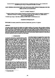
Fig. 9 Examples of normal and abnormal crowed activities in scenes of the UMN dataset. Top: Normal. Bottom: Abnormal

or a bicycle among the normal pedestrians is considered to be abnormal. All training frames in this dataset (Ped1 and Ped2) are normal when they contain pedestrians only. We evaluate our algorithm on both Ped1 and Ped2. – Ped1: There are 34 normal video samples for training and 36 abnormal video sequences for testing. There is no available ground truth for all video sequence in Ped1. Each sequences includes about 200 frames with resolution of 158 × 238. The total number of abnormal frames and normal frames are ≈ 3400 and ≈ 5000, respectively. – Ped2: Ped2 includes 12 and 16 video sequences for testing and training with resolution of 320 × 240. To evaluate the localization, the ground truth of all test frames is available. The total number of abnormal and normal frames are ≈ 2384 and ≈ 2566, respectively UMN [11] dataset has three different scenes. In each scene, a group of people walk in a region, suddenly all people scatter. This scattering (escape) is considered to be abnormal. Figure 9 illustrates examples of normal and abnormal frames of this dataset. This dataset has some limitations: there are only three abnormal scenes in the dataset. In addition, the temporal-spatial changes between normal and abnormal frames are very high. Also, UMN has no pixel-level ground truth. 5.3 Evaluation Methodology We compare our results with state-of-the-art methods using a receiver operating characteristic (ROC) curve, equal error rate (EER), detection rate (DR) and area under curve (AUC). For a better understanding in ROC, true positive rate (TPR) and false positive rate (FPR) terms should be introduced given ROC reflects their relationships. They are defined as: tp TPR = tp + f p (12) fp FPR = f p + tn

20

Mohammad Sabokrou, Mahmood Fathy, Zahra Moayed, and Reinhard Klette

where tp is true-positives, f p is false-positive and tn is the true-negative. We use two measures: at frame level and at pixel level which are introduced in [33] and exploited in the most of previous works. In addition to these measures, we define a new measure for the accuracy of anomaly localization, called dual pixel level. Based on these measures, the frames are considered to be abnormal (positive) or normal (negative). The measures that we use are as follows: 1. Frame level: In this measure, if one pixel shows an anomaly, then frame is considered to be abnormal [33]. 2. Pixel level: If at least 40 percent of abnormal ground truth pixels are shared with pixels that are detected by the algorithm, the frame is considered to be an abnormal [33]. 3. Dual pixel level: In this measure, a frame is considered to be abnormal if (1) it satisfies the abnormal condition at pixel level and (2) at least β percent (for example, 10 percent) of pixels detected as abnormal are similar with the abnormal ground truth. In addition to the abnormal regions, if irrelevant regions are also considered as abnormal, this measure does not identify the frame as being positive. In computer vision tasks for evaluating the localization performance, the labels of all detected pixels are compared pixel by pixel with the target labels of those pixels which are provided as ground truth. In this case, if the algorithm mistakenly detects a region as abnormal, all pixels of that region are considered as false positive. However, the pixel-level measure which is defined and used in state-of-the-art methods for anomaly localization just focuses on finding the location of anomaly. If the detected location in a frame is partially correct(i. e. have 40% overlap with exact pixels of anomaly), that frame is considered to be abnormal and all of false regions are ignored. Consequently, pixel-level measure does not care about regions which are wrongly detected as abnormal. It just checks to find the correct region among detected regions with respect to the ground-truths. To be sensitive to false region, we introduce the dual pixel-level measure. Suppose that the algorithm detects some regions as being abnormal and only one of these regions has an overlap with abnormal ground truth. Here, the number of false regions is not considered in the frame and pixel-level measures. Such a region is called a “lucky guess”. For considering the “lucky guess” region, we introduce the dual pixel level. This measure is sensitive to a “lucky guess”. Figure 10 shows an example for different measures of anomaly detection. 5.4 Performance The performance of the proposed algorithm is discussed in this section. 5.4.1 Influence of Patch Size and Patch Overlapping As mentioned in previous sections, we consider the video as being a set of cubic patches. The size of patches and level of overlapping in patches are two critical parameters which are related to video representation. As the final performance of system

Abnormal Behavior in Crowded Scenes

Anomaly

21

Anomaly

Normal

b

c

a

Anomaly

d

Fig. 10 Measure of anomaly evaluation. Blue and red rectangles indicate the output of the algorithm and abnormal ground truth, respectively. (a) Frame-level. (b) Pixel- level evaluation: 40 percent red (ground truth) is covered with blue (detected). (c) Dual pixel-level: Evaluates that 40 percent of red which are covered by blue, but at least β percent of blue is not covered by red. (d) Dual-pixel level . Table 1 Comparison of the accuracy and running time for different patch sizes Patch size Accuracy Time (second/frame)

20 94% 0.63

25 92% 0.42

30 87.2% 0.25

35 85% 0.20

40 76% 0.12

depends on these parameters, we run some experiments for concluding the optimum values. Our proposed algorithm is compatible to run with different patch sizes: 20, 25, 30, 35 and 40. Table 1 shows the effects of patch size on the frame level accuracy and the algorithm running time. Non-overlapped patches are exploited in this experiment. The accuracy is calculated using Equ (13). This experiment is applied on 4th video sub sequence of Ped2. Results show that decreasing the patch size leads to improving accuracy, but it has inverse relation with running time. A defines how accuracy is calculated for experimental results:

A=

tp + tn M

(13)

where M defines the number of samples. Effects of patch size on our method’s performance are evaluated. We also run our method with different levels of overlapping. The Results of ROC of frame-level of these experiments on Ped2 are shown in Figure 11. The results concludes that our proposed method achieves better performance by working with 40 × 40 × 5 extracted patches rather than working with 30×30×5 or 20×20×5 patches. Also, it has better performance than 50 × 50 × 5. We did same experiments on UMN and UCSD Ped2 benchmarks. Patches of size 40 × 40 × 5 outperforms the other sizes. The Figure 11 confirms that the patch extracting with more overlapping regions has given a better performance in frame level measure, but it is obvious that dense patch extraction is a time-consuming process.

22

Mohammad Sabokrou, Mahmood Fathy, Zahra Moayed, and Reinhard Klette

A

Distance

Fig. 11 Comparison of the ROC of frame level with different patch sizes and different level of overlapping for UCSD Ped2 Dataset. (Top-Left): patch size=50, overlapping size={5, 10, 15, 20, 25, 30, 35, 40}. (Top-Right): patch size=40, overlapping size={5, 10, 15, 20, 25, 30}. (Bottom-Left): patch size=30, overlapping size={5, 10, 15, 20, 25}. (Bottom-Right): patch size=20, overlapping size={5, 10, 15}. The large patches which are extracted densely (with high overlapping ) concludes best result. 100 90 80 70 60 50 40 30 20 10 0 1 5 9 13 17 21 25 29 33 37 41 45 49 53 57

The number of patche

16 17

C

Distance

B 100 90 80 70 60 50 40 30 20 10 0 1 5 9 13 17 21 25 29 33 37 41 45 49 53 57

The number of patche

Fig. 12 Steps of the proposed anomaly detector. (Top-left): Input frame of detector. Extracting 40×40 × 5 patches (Top-Right): The distance of all patches from C1 (the normal reference model).(Bottom-Right): The distance of remaining patches from global model.(Bottom-Left): The final output of system.

Abnormal Behavior in Crowded Scenes

23

5.4.2 Work-flow of Detection Figure 12 illustrates the work-flow of anomaly detection and localization. First, a video frame of size 158 × 238 is considered to be of size (158 − 20) × (238 − 20) and then it is converted to ≈ 30084 of 40 × 40 × 5 patches with 20 pixels overlapping. These patches are represented by local descriptor, and the distance of their description with the local reference model is calculated. As it is shown, the distance of many patches is less than 60. θ and α are set to 60 and 90, respectively. Consequently, those patches that have a distance less than 60 are considered as being strongly normal. In the next step, the strongly normal patches are ignored and just the remaining patches are considered for further checking. In this stage, the space search for anomaly are reduced from 60 to 18 samples. The 18 remaining patches which we can also named “challenging patches” are represented by the global descriptor, and the distance of these 18 patches from global model is calculated. For these models, θ and α are also adjusted to be 70 and 90, respectively. The distance of 16th and 17th is more than 90. So, they are labeled as strongly abnormal by global model. There are no patches which are labeled as strongly abnormal by a local model and weakly by the global model. Hence, just the 16th and 17th patch of the frame are abnormal in the output of the system. 5.4.3 Comparison with Other Methods Depends on experiments and a trade-offs between speed and accuracy, the patches dimension are selected to be (40 × 40 × 5) with 20 pixels overlapping. Some frame results on UCSD Ped1 dataset are shown in figure 13 (abnormal events are localized with green borders). Figure 13 confirms that the proposed method is able to detect and localize abnormal events efficiently. In addition, figure 14 shows a qualitative comparison with other methods on UCSD Ped2, in which the 1th and 2th columns are generated by temporal MDT and spatial MDT [33]. The 3rd , 4th , and 5th columns are given by MPPCA [35], social force [38] and optical flow [32], respectively. The two-right columns (6th and 7th ) are the results of our method, based on the global descriptor and joint (local and global) descriptors. In all three scenes, other methods are unable to detect the abnormal events or they detect some irrelevant regions as being abnormal. The Figure 14 indicates that our algorithm has the best performance either in anomaly detection or anomaly localization among the set of considered algorithms. For comparison, we take advantage of EER, DR and AUC of our method with most of state-of-the-art methods. Quantitative results in comparison with other proposed methods on Ped1 are provided in Table 2. The methods which are presented by Yuan et al. [55] and Xiao et al. [57] have the best performance among considered methods using frame level measure. Our method outperforms by 0.6% and 1.6% using two ideas, respectively. The DR of presented method is also better than all considered approach except [57]. Our method’s DR is 83.3% where the best result is 84%. [57] is based on learning patterns for each pixel. Working on pixel level pattern leads to better performance for localizing of the abnormal regions. However, as we

24

Mohammad Sabokrou, Mahmood Fathy, Zahra Moayed, and Reinhard Klette

Fig. 13 Examples of anomaly detection on UCSD Ped1. 40×40 × 5 patches when 20 pixels overlapping are considered. Temporal MDT

Spatial MDT

MPPC

Social force

Optic flow

Our method (global model)

Our method

Fig. 14 Example of anomaly detection from three scenes of Ped2. First column to 7th columns show the results for Temporal MDT, Spatial MDT, MPPCA, Social force, Optic flow, Our method (feature learning only) and Our method (combined views), respectively. In first five columns, the abnormal event pixels are colored in red; in 6th and 7th rows, the anomalies are localized with green and red borders, respectively. Table 2 Quantitative comparison of the proposed method and the state-of-the-art for anomaly detection using UCSD Ped1 dataset. EER and DR are exploited for Frame-Level and Pixel-Level, respectively. The 3rd column indicates the area of under the frame level ROC. The ”—” mark reveals the result is not reported by the reference paper. Method IBC [31] Adam et al. [32] SF [38] MPCCA+SF [33] Zaharescu et al. [39] MDT [33] Reddy et al. [65] SRC [1] STMC [45] Bertini et al. [8] Saligrama et al. [41] Dan Xu et al. 52% Nannan Li et al. [59] Weixin Li et al. [34] OADC-S [55] Tan Xiao et al. [57] iHOT [53] Dong-Gyu Lee et al. [58] Ours

EER 14% 38% 36% 32% 29% 25% 22.5% 19% 23% 31% 16% 85.4% 21% 17.8% 9% 10% 19.37% 24.1% 8.4%

DR 74% 24% 59% 18% 59% 42% 68% 46% 47% 30% —

AUC — 65.0% 67.0% 59.0% — 81.8% — 86% 86% —

63% 74.5% 74% 84% — 62% 83.3%

87.2% — 91 — — 64.9 93.2 %

Abnormal Behavior in Crowded Scenes

25

Table 3 Quantitative comparison of the proposed method and the state-of-the-art for anomaly detection using the UCSD Ped2 dataset. EER and DR are exploited for Frame-Level and Pixel-Level, respectively. The 3rd column indicates the area of under the frame level ROC. The ”—” mark reveals the result is not reported by the reference paper. EER 13% 42% 42% 36% 17% 24% 20% 30% 24.8% 18% 21% 20% 18.5% — 10% 19% 8.59% 9.8% 7.5%

100

100

90

90

80

80

70

70

60

60

TPR

TPR

Method IBC [31] Adam et al. [32] SF [38] MPCCA+SF [33] Zaharescu et al. [39] MDT [33] Reddy et al. [65] Bertini et al. [8] STMC [45] Saligrama et al. [41] Dan Xu et al. [51] Nannan Li et al. [59] Li et al. [34] OADC-S [55] Tan Xiao et al. [57] Sabokrou [9] iHOT [53] Dong-Gyu Lee et al. [58] Ours

50 40

DR 74% 24% 20% 28% 70% 46% — — — — — — 70.1% — 83% 76% – 78% 84%

AUC — 63% 63% 71% — 85% — — 86.8% 88.2% 89.1% — 92.5 — — – 81.5% 93.9 %

50 40

30

30

Sabokrou et al. MDT Dan Xua et al Proposed(Local threshold) Proposed(Overall threshold) EER curve

20 10 0 0

10

20

30

40

50

FPR

60

70

80

90

Sabokrou et al MDT Dan Xua et al Proposed(Overall threshold) Proposed(Local threshold) EER curve

20 10 100

0 0

10

20

30

40

50

FPR

60

70

80

90

100

Fig. 15 Comparison ROC curve Left: Frame-level evaluation Right: pixel- level evaluation

mentioned before, working with very small regions especially pixels instead of large patches causes to increase false positive rate which incurs inferior effects on framelevel performance. Although it works better in pixel-level measure, their method can not succeed as well as proposed method in frame-level measure. In Figure 15–left, the frame-level ROC of our method (with local and overall threshold) is compared with other methods on the Ped2 dataset. It shows that our method is highly comparable to other methods. However, the ROC of the proposed method with local threshold is superior to overall threshold case; our algorithm with overall threshold works like state-of-the-art method. As we tune and set the overall threshold (α and θ) once, it is faster in training and testing steps than local threshold. The 12 different subsequences of Ped2 do not have the same thresholds, but

26

Mohammad Sabokrou, Mahmood Fathy, Zahra Moayed, and Reinhard Klette

Table 4 EER of Dual pixel-level on UCSD dataset, and comparison with our previous work. Dual pixellevel and β are defined in section 5.3 Ped 1: Ped 2: Sabokrou et al.[9] Ped 2:

β=0 16.7% 16% 19%

β = 5% 26.2% 25.8% 27.5%

β = 10% 53.5% 49.2% 67.5%

as we attempt to have a high true positive in each model, the minimum value of thresholds which are calculated based on Equ. (7) and Equ. (7) are considered (as pre-processing, two thresholds for all 12 sequences are calculated and minimum is applied for all). The EER of frame level for different methods on Ped2 is shown in Table 3. It suggests that our method has a good performance compared with others. The methods which are reported by Tan Xiao et al. [57] and iHOT [53] have a close result to Ours, however, our method outperforms by 2.5% and 1.09%, respectively. Figure 15–Right is related to pixel-level ROC on Ped2. Our methods is superior compared with the other methods as well as frame-level measure. In Table 3 (3rd column), we compare the DR of our method with DR of other approaches. The calculated DR of our method is 84% where the next best result is 83% reported by Tan Xiao et al. [57]. Hence, Our method surpass other considered methods by 1% in DR. The ROC and DR results show that our algorithm outperforms other methods in the pixel-level measure. In addition, the AUC of proposed method has been compared with state-of-the-art methods. Table 2 and 3 indicate that similar to EER and DR measures, the AUC of our approach has higher performance compared to the best result of other considered methods by 1.2% and 1.4% on ped1 and ped2, respectively. We also use a dual-pixel level measure to analyze the accuracy of anomaly localization. Table 4 shows the effects of β on our algorithm. As we explained, the focus of this measure is on considering the regions which are falsely detected as abnormal. These regions are not considered in frame-level and pixel level evaluation. Our algorithm has achieved the goal of having superior performance, even higher than some state-of-the-art methods, in pixel level with β = 5% percent. The dual-pixel EER of our method (with β = 5%) on Ped1 and Ped2 are 26.2% and 25.8%, where it can be compared with the pixel-level of the other methods. This measure is introduced in this paper, the result of other algorithms with respect to this measure are not available, so just a comparison with our previous work [9] is done (see last row in Table 4). 5.4.4 Performance on UMN Dataset To evaluate our method in UMN dataset, EER and AUC in frame-level are used. EER and AUC results are shown in Table 5. As this dataset is simple and anomaly localization is not crucial, only the global detector is used. Previous methods performed perfectly on this dataset. The AUC of our method is comparable with previous methods, while the EER of our approach is better (by 0.3%) than the one of the best previous method.

Abnormal Behavior in Crowded Scenes

27

Table 5 Anomaly detection performance in EER and AUC Method Chaotic invariants [21] SF [38] Sparse [1] Saligrama et al. [41] Li et al. [34] Ours

EER 5.3 12.6 2.8 3.4 3.7 2.5

AUC 99.4 94.9 99.6 99.5 99.5 99.6

Table 6 Run time comparison, Hardware: PC with an Intel Q9550 CPU and 4 GB of RAM. Software:Matlab Method IBC MDT STC Ours(With 20 pixels overlapping ) Ours(Without overlapping)

Ped1 55 17 0.16 0.51 0.11

Ped2 66 23 0.18 0.63 0.13

5.4.5 Run-time Comparison The run-time is reported in state-of-the-art methods which are executed and implemented on different hardware and software. Consequently, comparing with all stateof-the art is somehow impossible. We just compare our algorithm with IBC[31], MDT[33] and STC[43] methods. This comparison is shown in Table 6. The reported results are the approximate computational time achieved on a PC with an Intel Q9550 CPU and 4 GB of RAM. If the patches of a frame are extracted with 20 pixels overlapping, the performance of our method is better than state-of the-art and we outperforms all methods. The results suggest that extracting patches without overlapping leads to a faster approach as it is shown in latest row of Table 6. So, with considering a bit error(≈ 5% EER) and optimizing the code, our approach is fast; we reach up to 25 fps(i. e. 0.04 second for each frame). We do not claim that the proposed method is real-time, but it is highly time-efficient.

5.5 Discussion Experimental results confirm that our method is comparable to state-of-the-art method in terms of both accuracy and time efficiency. The advantages of our method compared to previous methods are: (1) Focusing on fusion of two different representation of video where it leads to low false positive and high true positive for anomaly detection. Also, (2) the implementation of algorithm is easy, and (3) both spatial and temporal features are considered for representing the video. However the performance of the proposed algorithm is acceptable, it is not completely robust against some problem such as:

28

Mohammad Sabokrou, Mahmood Fathy, Zahra Moayed, and Reinhard Klette

1. perspective problem: In training data (i. e. normal videos), there are many close and far objects in patches respective to the cameras, so the normal reference model learns about different situation. We have found that considering a normal reference model for close objects and another one for far objects will lead to better performance. 2. By increasing the quality of video (size of the frame), this method performs slower than 25fps. In other works, the run-time of algorithm depends on the size of input video as well. 3. As a deep learning based method, proposing an end-to-end architecture is more interesting. 6 Conclusions In this work, we propose a patch-based anomaly detection and localization method based on representing a given video by using global and local descriptors. The main goal of the proposed descriptors is capturing and modeling the spatial-temporal context of a video. Those patches that occur rarely in the given video, and which differ compared to their adjacent patches are considered as abnormal. The relation of a patch to all the other patches, which are seen in a given video, is considered as a global descriptor. The structural similarity of a patch with adjacent patches defines a local descriptor. Two Gaussian classifiers are proposed based on these two forms of representations. For being accurate and fast, a cascaded structure is applied for fusing the results of the two descriptors as the final output of the system. Moreover, we introduced a new metric for region-level anomaly detection for suspicious regions. On the UCSD and UMN datasets, our method outperforms recent approaches. It is worth focusing on the fast anomaly detection in this paper. Acknowledgement This research was in part supported by a grant from IPM. (No. CS1396-5-01) References 1. Cong Y et al. (2011) Sparse reconstruction cost for abnormal event detection. In: CVPR’11. Proceedings of the 2011 IEEE Conference on Computer Vision and Pattern Recognition, pp 3449–3456 2. Krizhevsky A et al. (2012) Imagenet classification with deep convolutional neural networks. In: Advances Neural Information Processing Systems. pp 1097–1105 3. Girshick R et al. (2014) Rich feature hierarchies for accurate object detection and semantic segmentation. In: CVPR’14. IEEE Conference on Computer Vision and Pattern Recognition, Columbus, OH, June 2014, pp 580–587 4. Simonyan K, Zisserman A (2014) Two-stream convolutional networks for action recognition in videos. In: NIPS’14. Advances Neural Information Processing Systems, pp 68–576 5. Yang Y et al. (2013) Semi-supervised learning of feature hierarchies for object detection in a video. In: CVPR’13. IEEE Conference on Computer Vision and Pattern Recognition, Portland, OR, pp 1650–1657 6. Coates A et al. (2011) An analysis of single-layer networks in unsupervised feature learning. In: Proceedings of the fourteenth conference on Artificial Intelligence and Statistics, Fort Lauderdale, FL, USA, April 2011, pp 215–223

Abnormal Behavior in Crowded Scenes

29

7. Giusti A et al. (2013) Fast image scanning with deep max-pooling convolutional neural networks. In: ICIP’13. IEEE International Conference on Image Processing, Melbourne, VIC, pp 4034–4038 8. Bertini M, Del Bimbo A, Seidenari L (2012) Multi-scale and real-time non-parametric approach for anomaly detection and localization. Computer Vision and Image Understanding. 116(3):320–329 9. Sabokrou M et al. (2015) Real-time anomaly detection and localization in crowded scenes. In: CVPRW’15. IEEE Conference on Computer Vision and Pattern Recognition Workshops, Boston, MA, pp 320–329 10. Statistical Visual Computing Lab, UC San Diego (2013) UCSD Anomaly Detection Dataset. www. svcl.ucsd.edu/projects/anomaly/dataset.html. Accessed Feb. 2013 11. Artificial Intelligence, Robotics and Vision Laboratory University of Minnesota, Department of Computer Science and Engineering (2006) Monitoring Human Activity. mha.cs.umn.edu/Movies/ Crowd-Activity-All.avi. Accessed Feb. 2013 12. Lu C et al. (2013) Abnormal event detection at 150 fps in MATLAB. In: ICCV’13. IEEE International Conference on Computer Vision, Sydney, VIC, pp 2720–2727 13. Xu D et al. (2015) Learning deep representations of appearance and motion for anomalous event detection. In: BMVC’15. British Machine Vision Conference. 14. Vincent P et al. (2008) Extracting and composing robust features with denoising autoencoders. In: ICML ’08. Proceedings of the 25th international conference on Machine learning. ACM, New York, NY, USA, pp 1096–1103 15. Ravanbakhsh M et al. (2016) Plug-and-Play CNN for Crowd Motion Analysis: An Application in Abnormal Event Detection. In: arXiv preprint arXiv:1610.00307 16. Zhou S et al. (2016) Spatialtemporal convolutional neural networks for anomaly detection and localization in crowded scenes. In: Signal Processing: Image Communication, pp 358–368 17. Hu X et al. (2016) Video anomaly detection using deep incremental slow feature analysis network. In: IET Computer Vision, Vol 10, pp 258–265 18. Fang Z et al. (2016) Abnormal event detection in crowded scenes based on deep learning. In: Multimedia Tools and Applications, Vol 75, pp 14617–14639 19. Munwar A, Vinayavekhin P, Magistris G(2017) Spatio-Temporal Anomaly Detection for Industrial Robots through Prediction in Unsupervised Feature Space. In: IEEE Winter Conference on Applications of Computer Vision (WACV 2017). 20. Jianga F, Yuan J, Tsaftarisa S A, Katsaggelosa A K (2011) Anomalous video event detection using spatiotemporal context. Computer Vision and Image Understanding. 115(3):323–333 21. Wu S et al. (2010) Chaotic invariants of Lagrangian particle trajectories for anomaly detection in crowded scenes. In: CVPR’10. IEEE Conference on Computer Vision and Pattern Recognition, San Francisco, CA, pp 2054–2060 22. Piciarelli C, Micheloni C, Foresti G L (2008) Trajectory-based anomalous event detection. IEEE Transactions on Circuits and Systems for Video Technology. 18(11): 1544–1554 23. Antonakaki P, Kosmopoulos D, Perantonis S J (2009) Detecting abnormal human behaviour using multiple cameras. Signal Processing. 89(9):1723–1738 24. Calderara S, Heinemann U, Prati A et al. (2011) Detecting anomalies in people’s trajectories using spectral graph analysis. Computer Vision Image Understanding. 115(8):1099–1111 25. Morris B T, Trivedi M M (2011) Trajectory learning for activity understanding: Unsupervised, multilevel, and long-term adaptive approach. IEEE Transactions on Pattern Analysis Machine Intelligence. 33(11):2287–2301 26. Biswas S, Rabu v (2017) Anomaly detection via short local trajectories Neurocomputing. 242:6372 27. Hu W, Xiao X, Fu Z et al. (2006) A system for learning statistical motion patterns. IEEE Transactions on Pattern Analysis Machine Intelligence. 28(9):1450–1464 28. Tung F, Zelek J S, Clausi D A (2011) Goal-based trajectory analysis for unusual behaviour detection in intelligent surveillance. Image Vision Computing. 29(4):230–140 29. Piciarelli C, Foresti GL (2006) On-line trajectory clustering for anomalous events detection. Pattern Recognition Letters. 27(15):1835–1842, 2006. 30. Zhang D et al. (2005) Semi-supervised adapted HMMS for unusual event detection. In: CVPR’05. IEEE Conference on Computer Vision and Pattern Recognition, Vol 1, p 611–618 31. Boiman O, Irani M (2007) Detecting irregularities in images and in video. International Journal of Computer Vision. 74(1):17–31 32. Adam A, Rivlin E, Shimshoni I,Reinitz D (2008) Robust real-time unusual event detection using multiple fixed location monitors. IEEE Transactions on Pattern Analysis Machine Intelligence. 30(3):555– 560

30

Mohammad Sabokrou, Mahmood Fathy, Zahra Moayed, and Reinhard Klette

33. Mahadevan V et al. (2010) Anomaly detection in crowded scenes. In: CVPR’10. IEEE Conference on Computer Vision and Pattern Recognition. San Francisco, CA, pp 1975–1981 34. Li W, Mahadevan V, Vasconcelos N (2014) Anomaly detection and localization in crowded scenes. IEEE Transactions on Pattern Analysis Machine Intelligence. 36(1):18–32 35. Kim J, Grauman K (2009) Observe locally, infer globally: a space-time MRF for detecting abnormal activities with incremental updates. In: CVPR’09. IEEE Conference on Computer Vision and Pattern Recognition. Miami, FL, pp 2921–2928 36. Benezeth Y et al. (2009) Abnormal events detection based on spatio-temporal co-occurrences. In: CVPR’09. IEEE Conference on Computer Vision and Pattern Recognition. Miami, FL, pp 1446–1453 37. Kratz L, Nishino K (2009) Anomaly detection in extremely crowded scenes using spatio-temporal motion pattern models. In: CVPR’09. IEEE Conference on Computer Vision and Pattern Recognition. Miami, FL, pp 1446–1453 38. Mehran R et al. (2009) Abnormal crowd behavior detection using social force model. In: CVPR’09. IEEE Conference on Computer Vision and Pattern Recognition. Miami, FL, pp 935–942 39. Zaharescu A, Wildes R (2010) Anomalous behaviour detection using spatiotemporal oriented energies, subset inclusion histogram comparison and event-driven processing. In: ECCV’10. Proceedings of the 11th European conference on Computer vision. Springer-Verlag, Berlin, Heidelberg, pp 563–576 40. Anti´c B, Ommer B (2011) Video parsing for abnormality detection In: ICCV’11. International Conference on Computer Vision. Barcelona, pp 2415–2422 41. Saligrama V and Chen Z (2012) Video anomaly detection based on local statistical aggregates. In: CVPR’12. IEEE Conference on Computer Vision and Pattern Recognition, Providence, RI, pp 2112– 2119 42. Ullah H, Conci N (2012) Crowd motion segmentation and anomaly detection via multi-label optimization. In: ICPR’12. ICPR Workshop Pattern Recognition Crowd Analysis. Japan. 43. Roshtkhari M J, Levine M D (2013) An on-line, real-time learning method for detecting anomalies in videos using spatio-temporal compositions. Computer Vision Image Understanding. 117(10):1436– 1452 44. Zhu Y et al. (2013) Context-aware modeling and recognition of activities in video. In: CVPR’13. IEEE Conference on Computer Vision and Pattern Recognition. Portland, OR, pp 2491–2498 45. Cong Y, Yuan J, Tang Y (2013) Video anomaly search in crowded scenes via spatio-temporal motion context. IEEE Transactions on Information Forensics Security. 8(10):1590–1599 46. Roshtkhari M J, Levine MD (2013) Online dominant and anomalous behavior detection in videos. In: CVPR’13. IEEE Conference on Computer Vision and Pattern Recognition. Portland, OR, pp 2611–2618 47. Nakahata M T. et al (2017) Anomaly detection with a moving camera using spatio-temporal codebook. In: Multidimensional Systems and Signal Processing, pp 1–30 48. Ullah H, Tenuti L, Conci N (2013) Gaussian mixtures for anomaly detection in crowded scenes. In: Proceeding IS&T/SPIE Electronic Imaging. Burlingame, California, USA, Vol 8663 49. Ullah H, Tenuti L, Conci N (2014) Real-time anomaly detection in dense crowded scenes. In: Proceeding IS&T/SPIE Electronic Imaging. San Francisco, California, United States, Vol 9026 50. Ullah H, Tenuti L, Conci N (2014) Dominant motion analysis in regular and irregular crowd scenes. In: HBU’14. Proceedings of ECCV workshop on Human behaviour Understanding. Zurich, Switzerland, pp 62–72 51. Xu D, Song R, Wu X et al. (2014) Video anomaly detection based on a hierarchical activity discovery within spatio-temporal contexts. Neurocomputing. 143:144–152, 2014. 52. Mousavi H et al. (2015) Analyzing tracklets for the detection of abnormal crowd behavior. In: IEEE Winter Conference on Applications of Computer Vision, pp 148–155 53. Mousavi H et al. (2015) Abnormality detection with improved histogram of oriented tracklets. In: ICIAP’15. International Conference on Image Analysis and Processing, Italy, Vol 9280, pp 722–732 54. Rabiee H. et al. (2017) Detection and localization of crowd behavior using a novel tracklet-based mode. In: International Journal of Machine Learning and Cybernetics, pp 1–12 55. Yuan Y, Fang J, Wang Q (2015) Online anomaly detection in crowd scenes via structure analysis. IEEE Transactions on Cybernetics. 45(3):562–575 56. Cheng K W et al. (2015) Video anomaly detection and localization using hierarchical feature representation and Gaussian process regression. In: CVPR’15. IEEE Conference on Computer Vision and Pattern Recognition. Boston, MA, pp 2909–2917 57. Xiao T, Zhang C, Zha H (2015) Learning to detect anomalies in surveillance video. IEEE Signal Processing Letters. 22(9):1477–1481

Abnormal Behavior in Crowded Scenes

31

58. Lee D, Suk H I, Park S K et al. (2015) Motion influence map for unusual human activity detection and localization in crowded scenes. IEEE Transactions on Circuits Systems Video Technology. 25(10):16121623 59. Li N, Wu X, Xu D et al. (2015) Spatio-temporal context analysis within video volumes for anomalousevent detection and localization. Neurocomputing. 155:309–319 60. Sabokrou M et al. (2016) Video anomaly detection and localisation based on the sparsity and reconstruction error of auto-encoder. In: Electronics Letters, Vol 52, pp 1122–1124 61. Sabokrou M et al. (2017) Deep-Cascade: Cascading 3D Deep Neural Networks for Fast Anomaly Detection and Localization in Crowded Scenes. In: IEEE Transactions on Image Processing, vol. 26, no. 4, pp 1992–2004 62. Sabokrou M et al. (2017) Deep-Anomaly: Fully Convolutional Neural Network for Fast Anomaly Detection in Crowded Scenes. In: CoRR 63. Brunet D, Vrscay E R, Wang Z (2012) On the mathematical properties of the structural similarity index. IEEE Transactions on Image Processing. 21(4):1488–1499 64. Wang Z, Bovik A C, Sheikh H R et al. (2004) Image quality assessment: from error visibility to structural similarity. IEEE Transactions on Image Processing. 13(4):600–612 65. Reddy V et al. (2011) Improved anomaly detection in crowded scenes via cell-based analysis of foreground speed, size and texture. In: CVPR Workshops. Colorado Springs, CO, pp 55–61