assignment is inconsistent, the DPLL procedure backtracks just as it would if an empty clause were detected. In addition, a central feature of DPLL(T) is.
Fast and Flexible Difference Constraint Propagation for DPLL(T) Scott Cotton and Oded Maler ´ Verimag, Centre Equation 2, Avenue de Vignate 38610 Gi`eres, France {Scott.Cotton,Oded.Maler}@imag.fr
Abstract. In the context of DPLL(T), theory propagation is the process of dynamically selecting consequences of a conjunction of constraints from a given set of candidate constraints. We present improvements to a fast theory propagation procedure for difference constraints of the form x − y ≤ c. These improvements are demonstrated experimentally.
1
Introduction
In this paper, theory propagation refers to the process of of dynamically selecting consequences of a conjunction of constraints from a given set of constraints whose truth values are not yet determined. The problem is central to an emerging method, known as DPLL(T) [10, 17, 3, 18] for determining the satisfiability of arbitrary Boolean combinations of constraints. We present improvements to theory propagation procedure for difference logic whose atomic constraints are of the form x − y ≤ c. Our contribution is summarized below: 1. We introduce flexibility in the invocation times and scope of constraint propagation in the DPLL(T) framework. This feature is theory independent and is described in more detail in [4]. 2. We identify conditions for early termination of single source shortest path (SSSP) based incremental propagation. These conditions allow us to ignore nodes in the constraint graph which are not affected by the assignment of the new constraint. 3. We implement a fast consistency check algorithm for difference constraints based on an algorithm presented in [9]. As a side effect, the performance of subsequent theory propagation is improved. We present an adaptation of Goldberg’s smart-queue algorithm [11] for the theory propagation itself. 4. We show that incremental complete difference constraint propagation can be achieved in O(m + n log n + |U |) time, where m is the number of constraints whose consequences are to be found, n the number of variables in those constraints, and U the set of constraints which are candidates for being deduced. This is a major improvement over the O(mn) complexity of [17].
The rest of this paper is organized as follows. In Section 2 we describe the context of theory propagation in DPLL(T) and review difference constraint propagation in particular. In Section 3, we present a simplified consistency checker which also speeds up subsequent propagation. Our propagation algorithm including the early termination feature is presented in Section 4; experimental evidence is presented in Section 5; and we conclude in Section 6.
2
Background
Propagation in DPLL(T) The Davis-Putnam-Loveland-Logemann (DPLL) satisfiability solver is concerned with propositional logic [6, 5]. Its input formula ϕ is assumed to be in conjunctive normal form. Given such a formula, a DPLL solver will search the space of truth assignments to the variables by incrementally building up partial assignments and backtracking whenever a partial assignment falsifies a clause. Assignments are extended both automatically by unit propagation and by guessing truth values. Unit propagation is realized by keeping track of the effect of partial assignments on the clauses in the input formula. For example, the clause x ∨ ¬y is solved under an assignment including y 7→ false and is reduced to the clause x under an assignment which includes y 7→ true but which contains no mapping for x. Whenever a clause is reduced to contain a single literal, i.e. it is in the form v or the form ¬v, the DPLL engine extends the partial assignment to include the truth value of v which solves the clause. If a satisfying assignment is found, the formula is satisfiable. If the procedure exhausts the (guessed) assignment space without finding a satisfying assignment, the formula is not satisfiable. DPLL(T) is a DPLL-based decision procedure for satisfiability modulo theories. The DPLL(T) framework extends a DPLL solver to the case of a Boolean combination of constraints which are interpreted with respect to some background theory T . An external theory-specific solver called SolverT is invoked at each assignment extension in the DPLL procedure. SolverT is responsible for checking the consistency of the assignment with respect to the theory T . If an assignment is inconsistent, the DPLL procedure backtracks just as it would if an empty clause were detected. In addition, a central feature of DPLL(T) is that SolverT may also find T -consequences of the assignment and communicate them to the DPLL engine. This latter activity, called theory propagation, is intended to help guide the DPLL search so that the search is more informed with respect to the underlying theory. Theory propagation is thus interleaved with unit propagation and moreover the two types of propagation feedback into one another. This quality gives the resulting system a strong potential for reducing the guessing space of the DPLL search. Consequently, DPLL(T) is an effective framework for satisfiability modulo theories [10, 3, 17]. Flexible Propagation We define an interface to SolverT which allow it to interact with the DPLL engine along any such interleaving of unit propagation and theory propagation. Below are three methods to be implemented by SolverT , which can be called in any sequence:
SetTrue. This method is called with a constraint c every time the DPLL engine extends the partial assignment A with c. SolverT is expected to indicate whether or not A∪{c} is T -consistent. If consistent, an empty set is returned. Otherwise, an inconsistent subset of A ∪ {c} is returned. TheoryProp. This method returns a set C of T -consequences of the current assignment A. A set of reasons Rc ⊆ A is associated with each c ∈ C, satisfying Rc |= c. Unlike the original DPLL(T) of [10], the method is entirely decoupled from SetTrue. Backtrack. This method simply indicates which assigned constraints become unassigned as a result of backtracking. The additional flexibility of the timing of occurences of calls to SetTrue in relation to occurences of calls to TheoryProp allows the system to propagate constraints either eagerly or lazily. Eager propagation follows every call to SetTrue with a call to TheoryProp. Lazy propagation calls TheoryProp only after a sequence of calls to SetTrue, in particular when unit propagation is not possible. Whatever the sequence of calls, it is often convenient to identify the source of an assignment in the method SetTrue. At the same time, it is the DPLL engine which calls these methods and we would like to minimize its responsibilities to facilitate using off-the-shelf DPLL solvers along with the host of effective optimizations associated with them. Hence, we do not require that the DPLL engine keep track of the source of every assignment. Rather we allow it to treat constraints more or less the same way it treats propositional literals, and put the burden on SolverT instead. Towards this end, we have SolverT associate an annotation αc with each constraint (or its negation) which appears in a problem. In addition to tracking the origin of constraints passed to SetTrue, the annotation is used to keep track of a set of assigned constraints whose consequences have been found. The annotation can take any value from {Π, Σ, ∆, Λ} with the following intended meanings. Π: Constraints whose consequences have been found (propagated constraints). ∆: Constraints which have been identified as consequences of constraints labelled Π. Σ: Constraints which have been assigned, but whose consequences have not been found yet. Λ: Unassigned constraints. For convenience, we use the labels Π, ∆, Σ and Λ interchangeably with the set of constraints which have the respective label. It is fairly straightforward to maintain labels with these properties via the methods SetTrue, TheoryProp, and Backtrack. Whenever a constraint is passed to SetTrue which is labelled Λ we label it Σ and perform a consistency check. Whenever TheoryProp is called, constraints labelled Σ are labelled Π one at a time. After each such relabelling, all the constraints in Σ ∪ Λ which are consequences of constraints labelled Π are re-labelled ∆. Whenever backtracking
occurs, all constraints which become unassigned together with all consequences which are not yet assigned are labelled Λ. As explained at length in [4] for the more general context of theory decomposition, such constraint labels provide for a more flexible form of theory propagation which, in particular, exempts constraints labelled ∆ from consistency checks and from participating as antecedents in theory propagation. This feature reduces the cost of theory propagation without changing its outcome, and is independent of the theory and propagation method used. 2.1
Difference Constraints and Graphs
Difference constraints can express naturally a variety of timing-related problems including schedulability, circuit timing analysis, and bounded model checking of timed automata [16, 3]. In addition, difference constraints can be used as an abstraction for general linear constraints and many problems involving general linear constraints are dominated by difference constraints. Difference constraints are also much more easily decided than general linear constraints, in particular using the following convenient graphical representation. Definition 1 (Constraint graph). Let S be a set of difference constraints and c let G be the graph comprised of one weighted edge x → y for every constraint x − y ≤ c in S. We call G the constraint graph of S. The constraint graph may be readily used for consistency checking and constraint propagation, as is indicated in the following well-known theorem. Theorem 1. Let Γ be a conjunction of difference constraints, and let G be the constraint graph of Γ . Then Γ is satisfiable if and only if there is no negative cycle in G. Moreover, if Γ is satisfiable, then Γ |= x − y ≤ c if and only if y is reachable from x in G and c ≥ dxy where dxy is the length of a shortest path from x to y in G. As the semantics of conjunctions of difference constraints are so well characterized by constraint graphs, we refer to sets of difference constraints interchangeably with the corresponding constraint graph. In this way, we also further abuse the notation associated with constraint labels introduced in section 2. In particular, the labels Π, Σ, ∆, and Λ are used not only to refer to the set of difference constraints with the respective label, but also to the constraint graph induced by that set of constraints. We also often refer to a difference constraint c x − y ≤ c by an edge x → y in a constraint graph and vice versa.
3
Consistency Checks
In accordance with Theorem 1, one way to show that a set of difference constraints Γ is consistent is to show that Γ ’s constraint graph G contains no negative cycle. This in turn can be accomplished by establishing a valid potential function, which is a function π on the vertices of a graph satisfying c π(x) + c − π(y) ≥ 0 for every edge x → y in G. A valid potential function
may readily be used to establish lower bounds on shortests path lengths between arbitrary vertices (v1 , vn ): n−1 Σi=1 π(vi ) + ci − π(vi+1 ) ≥ 0 n−1 π(v1 ) − π(vn ) + Σi=1 ci ≥ 0 n−1 Σi=1 ci ≥ π(vn ) − π(v1 )
If one considers the case that v1 = vn , it follows immediately that the existence of a valid potential function guarantees that G contains no negative cycles. In addition, a valid potential function for a constraint graph G defines a satisfying assignment for the set Γ of difference constraints used to form G. In particular, if π is a valid potential function for G, then the function v 7→ −π(v) is a satisfying assignment for Γ . In the DPLL(T) framework, consistency checks occur during calls to SetTrue, d
when a constraint u → v is added to the set of assigned constraints. If the constraint is labelled ∆, then there is no reason to perform a consistency check. Otherwise, the constraint is labelled Σ. In this latter case, SetTrue must perform a consistency check on the set Π ∪Σ. To solve this problem, we make use of an incremental consistency checking algorithm based largely on an incremental shortests paths and negative cycle detection algorithm due to Frigioni1 et al [9]. Before detailing this algorithm, we first formally state the incremental consistency checking problem in terms of constraint graphs and potential functions: Definition 2 (Incremental Consistency Checking). Given a directed graph G with weighted edges, a potential function π satisfying π(x) + c − π(y) ≥ 0 for c d every edge x → y, and an edge u → v not in G, find a potential function π ′ for d the graph G′ = G ∪ {u → v} if one exists. The complete algorithm for this problem is given in pseudocode in Figure 1. The algorithm maintains a function γ on vertices which holds a conservative estimate on how much the potential function must change if the set of constraints is consistent. The function γ is refined by scanning outgoing edges from vertices for which the value of π ′ is known. 3.1
Proof of Correctness and Run Time
Lemma 1. The value min(γ) is non-decreasing throughout the procedure. Proof. Whenever the algorithm updates γ(z) to γ ′ (z) 6= γ(z) for some vertex z, it does so either with the value 0, or with the value π ′ (s) + c − π(t) for some c edge s → t in G such that t = z. In the former case, we know γ(z) < 0 by the termination condition, and in the latter we have γ ′ (z) = π ′ (s) + c − π(t) = (π(s) + c − π(t)) + γ(s) ≥ γ(s), since π(s) + c − π(t) ≥ 0. ⊓ ⊔ 1
The algorithm and its presentation here are much simpler primarily because Frigioni et al. maintain extra information in order to solve the fully dynamic shortests paths problem, whereas this context only demands incremental consistency checks. In particular, we do not compute single source shortests paths, but rather simply use a potential function which reduces the graph size.
γ(u) ← π(u) + d − π(v) γ(w) ← 0 for all w 6= v while min(γ) < 0 ∧ γ(u) = 0 s ← argmin(γ) π ′ (s) ← π(s) + γ(s) γ(s) ← 0 c for s → t ∈ G do if π ′ (t) = π(t) then γ(t) ← min{γ(t), π ′ (s) + c − π(t)} Fig. 1. Incremental consistency checking algorithm, invoked by SetTrue for a cond straint u → v labelled Λ. If the outer loop terminates because γ(u) < 0, then the set of difference constraints is not consistent. Otherwise, once the outer loop terminates, π ′ is a valid potential function and −π ′ defines a satisfying assignment for the set of difference constraints.
Lemma 2. Assume the algorithm is at the beginning of the outer loop. Let z be any vertex such that γ(z) < 0. Then there is a path from u to z with length L(z) = π(z) + γ(z) − π(u). Proof. (sketch) By induction on the number of times the outermost loop is executed. ⊓ ⊔ Theorem 2. The algorithm correctly identifies whether or not G′ contains a negative cycle. Moreover, when there is no negative cycle the algorithm establishes a valid potential function for G′ . Proof. We consider the various cases related to termination. – Case 1. γ(u) < 0. From this it follows that L(u) < 0 and so there is a negative cycle. In this case, since the DPLL engine will backtrack, the original potential function π is kept and π ′ is discarded. – Case 2. min(γ) = 0 and γ(u) = 0 throughout. In this case we claim π ′ is a valid potential function. Let γi be the value of γ at the beginning of the ith iteration of the outer loop. We bserve that ∀v . π ′ (v) ≤ π(v) and consider the following cases. • For each vertex v such that π ′ (v) < π(v), π ′ (v) = π(v) + γi (v) for c some refinement step i. Then for every edge v → w ∈ G, we have that ′ ′ γi+1 (w) ≤ π (v) + c − π(w) and so π (w) ≤ π(w) + γi+1 (w) ≤ π(w) + π ′ (v) + c − π(w) = π ′ (v) + c. Hence π ′ (v) + c − π ′ (w) ≥ 0. • For each vertex v such that π ′ (v) = π(v), we have π ′ (v) + c − π ′ (w) = c π(v) + c − π ′ (w) ≥ π(v) + c − π(w) ≥ 0 for every v → w ∈ G We conclude π ′ is a valid potential function with respect to all edges in G′ . In all cases, the algorithm either identifies the presence of a negative cycle, or it establishes a valid potential function π ′ . As noted above, a valid potential function precludes the existence of a negative cycle. ⊓ ⊔
Theorem 3. The algorithm runs in time2 O(m + n log n). Proof. The algorithm scans every vertex once. If a Fibonacci heap is used to find argmin(γ) at each step, and for decreases in γ values, then the run time is O(m + n log n). ⊓ ⊔ 3.2
Experiences and Variations
For simplicity, we did not detail how to identify a negative cycle if the set of constraints is inconsistent. A negative cycle is a minimal inconsistent set of constraints and is returned by SetTrue in the case of inconsistency. Roughly c speaking, this can be accomplished by keeping track of the last edge x → y along which γ(y) was refined for every vertex. Then every vertex in the negative cycle will have such an associated edge, those edges will form the negative cycle and may easily recovered. In practice we found that the algorithm is much faster if we maintain for each vertex v a bit indicating whether or not its new potential π ′ (v) has been found. With this information at hand, it is straightforward to update a single potential function rather than keeping two. In addition, this information can readily be used to skip the O(n) initialization of γ and to keep only vertices v with γ(v) < 0 in the priority queue. We found that the algorithm ran faster with a binary priority queue than with a Fibonacci heap, and also a bit faster when making use of Tarjan’s subtree-enumeration trick [20, 1] for SSSP algorithms. Profiling benchmark problems each of which invokes hundreds of thousands of consistency checks indicated that this procedure was far less expensive than constraint propagation in the DPLL(T) context, although the two have similar time complexity.
4
Propagation
The method TheoryProp described in Section 2 is responsible for constraint propagation. The procedure’s task is to find a set of consequences C of the current assignment A, and a set of reasons Rc for each consequence c ∈ C. For difference constraints, by Theorem 1, this amounts to computing shortests paths in a constraint graph. We present a complete incremental method for difference constraint propagation which makes use of the constraint labels Π, Σ, ∆, and Λ. The constraint propagation is divided into incremental steps, each of which selects a constraint c labelled Σ, relabels c with Π, and then finds the consequences of those constraints labelled Π from the set Σ ∪ Λ, labelling them ∆. A single step may or may not find unassigned consequences. On every call to TheoryProp, these incremental steps occur until either there are no constraints labelled Σ, or some unassigned consequences are found. Any unassigned consequences are returned to the DPLL(X) engine for assignment and further unit propagation. We state 2
Whenever stating the complexity of graph algorithms, we use n for the number of vertices in the graph and m for the number of edges.
the problem of a single incremental step in terms of constraint graphs and shortests paths below. Definition 3 (Incremental complete difference constraint propagation). c Let G, H be two edge disjoint constraint graphs, and let x → y ∈ H be a distind guished edge. Suppose that for every edge u → v ∈ H, the length of a shortest c c ′ path from u to v in G exceeds d. Let G = G ∪ {x → y} and H ′ = H \ {x → y}. d
Find the set of all edges u → v in H ′ such that the length of a shortest path from u to v in G′ does not exceed d. The preconditions relating the graphs G and H are a result of labelling and complete propagation. If all consequences of G are found and removed from H prior to every step, then no consequnces of G are found in H and so the length d of a shortest path from x to y in G exceeds the weight of any edge u → v ∈ H. As presented by Nieuwenhuis et al. [17], this problem may be reduced to solving two SSSP problems. First, for the graph G′ , the SSSP weights δy→ from y are computed and then SSSP weights δx← to x are computed, the latter being accomplished simply by computing δx→ in the reverse graph. Then for any cond
straint u → v ∈ H ′ , the weight of the shortests path from u to v passing through c x → y in G′ is given in constant time by δx← (u) + c + δy→ (v). In accordance with Theorem 1, the weight of this path determines whether or not the constraint d u → v is implied, in particular by the condition δx← (u) + c + δy→ (v) ≤ d. It then suffices to check every constraint in H ′ in this fashion. We now present several improvements to this methodology. 4.1
Completeness, Candidate Pruning, and Early Termination
A slight reformulation of the method above allows for early termination of the SSSP computations under certain conditions. That is, nodes for which it becomes clear that their minimal distance will not be improved due to the insertion of c x → y to the constraint graph will not be explored. We introduce the idea of relevancy below to formalize how we can identify such vertices and give an c example in Figure 2. For a new edge x → y, relevancy is based on shortest path distances δx→ (from x) and δy← (to y), in contrast to the formulation above. Under c this new formulation, if the shortest path from u to v passes through x → y, ← → then the path length is δy (u) + δx (v) − c. c
Definition 4 (δ-relevancy with respect to x → y). A vertex z is δx→ c relevant if every shortest path from x to z passes through x → y; similarly, a c vertex z is δy← -relevant if every shortest path from z to y passes through x → y. d
A constraint u → v is δ-relevant if both u is δy← -relevant and v is δx→ -relevant. d
A set C of constraints is δ-relevant if every u → v ∈ C is δ-relevant. Lemma 3. The solution set for complete incremental difference constraint propagation is δ-relevant.
X
Y
Z
Fig. 2. An example graph showing δ-relevant vertices with respect to the edge (x, y). For simplicity, all edges are assumed to have weight 1. The relevant vertices are white and the irrelevant vertices are shaded. As an example, the vertex z is not δx→ -relevant because there is a shortest path from x to z which does not pass through y. As a result, d any constraint u → z ∈ H ′ is not member of the incremental complete propagation solution set. c
Proof. Let x → y be the new edge in G, and suppose for a contradiction that d some constraint u → v ∈ H ′ in the solution set is not δ-relevant. Then the length of a shortest path from u to v in G′ does not exceed d. By definition of c δ-relevancy, some path p from u to v in G′ which does not pass through x → y is c at least as short as the shortest path from u to v passing through x → y. Observe d that p is a path in G. By the problem definition, u → v 6∈ H and H ′ ⊂ H. Hence d u → v 6∈ H ′ , a contradiction. ⊓ ⊔ Corollary 1 (Early Termination). It suffices to check every δ-relevant member of H ′ for membership in the solution set. As a result, each SSSP algorithm computing δ ∈ {δx→ , δy← } need only compute correct shortests path distances for δ-relevant vertices. Early termination is fairly easy to implement with most SSSP algorithms in the incremental constraint propagation context. First, for δ ∈ {δx→ , δy← }, we maintain a label for each vertex indicating whether or not it is δ-relevant. We then define an order ≺ over shortest path distances of vertices in a way that favors irrelevancy: δ(u) = δ(v) u is δ-irrelevant δ(u) ≺ δ(v) ⇐⇒ δ(u) < δ(v) or v is δ-relevant c
Since the new constraint x → y is a unique shortest path, we initially give y the label δx→ -relevant and x the label δy← -relevant. During the SSSP computation of d
δ, whenever an edge u → v is found such that δ(u) ≺ δ(v) + d, the distance to v is updated and we propagate u’s δ-relevancy label to v. If at any point in time all such edges are not δ-relevant, then the algorithm may terminate. To facilitate checking only δ-relevant constraints in H ′ , one may adopt a trick described in [17] for checking only a reachable subset of H ′ . In particular, one
may maintain the constraint graph H ′ in an adjacency list form which allows iteration over incoming and outgoing edges for each vertex as well as finding the in- and out-degree of each vertex. If the sets of δx→ -relevant and δy← -relevant vertices are maintained during the SSSP algorithm, the smaller of these two sets, measured by total in- or out-degree in H ′ , may be used to iterate over a subset of constraints in H ′ which need to be checked. 4.2
Choice of Shortests Path Algorithm
There are many shortest path algorithms, and it is natural to ask which one is best suited to this context. An important observation is that whenever shortests paths δx→ or δy← are computed, the graph G has been subject to a consistency check. Consistency checks establish a potential function π which can be used to speed up the shortests path computations a great deal. In particular, as was first observed by Johnson [13], we can use π(x)+c−π(y) as an alternate, non-negative c edge weight for each edge x → y. This weight is called the reduced cost of the edge. The weight w of path p from a to b under reduced costs is non-negative and the original weight of p, that is, without using reduced costs, is easily retrieved as w + π(b) − π(a). Our implementation of constraint propagation exploits this property by using an algorithm for shortests paths on graphs with non-negative edge weights. The most common such algorithm is Dijkstra’s [7], which runs in O(m + n log n) time. This is an improvement over algorithms which allow arbitrary edge weights, the best of which run in O(mn) time [2]. A direct result follows. Theorem 4. Complete incremental difference constraint propagation can be accomplished in O(m + n log n + |H ′ |) time where m is the number of assigned constraints, n the number of variables occuring in assigned constraints, and H ′ is the set of unassigned constraints. Proof. The worst case execution time of finding all consequences over a sequence of calls to SetTrue and TheoryProp, is O(m + n log n + |H ′ |) per call to TheoryProp and O(m + n log n) per call to SetTrue. Thus if every call to SetTrue is followed by a call to TheoryProp, then the combined time for both calls is O(m + n log n + |H ′ |). ⊓ ⊔ 4.3
Adaption of a Fast SSSP Algorithm
In order to fully exploit the use of the potential function in constraint propagation, we make use of a state-of-the-art SSSP algorithm for a graph with nonnegative edge weights. In particular, we implemented (our own interpretation of) Goldberg’s smart-queue algorithm [11]. The application of this algorithm to difference constraint propagation context is non-trivial because it makes use of a heuristic requiring that we keep track of some information for each vertex as the graph Π and its potential function changes. Even in the face of the extra book-keeping the algorithm turns out to run significantly faster than standard implementations of Dijkstra’s algorithm with a Fibonacci heap or a binary priority queue.
The smart-queue algorithm is a priority queue based SSSP algorithm for a graph with non-negative edge weights which maintains a priority queue on vertices. Each vertex is prioritized according to the shortest known path from the source to it. The smart-queue algorithm also makes use of the caliber heuristic which maintains for each vertex the minimum weight of any edge leading to it. This weight is called the caliber of the vertex. After removing the minimum element of distance d from the priority queue, d serves as a lower bound on the distance to all remaining vertices. When scanning a vertex, we know the lower bound d, and if we come accross a vertex v with caliber cv and tentative distance dv , we know that the distance dv is exact if d + cv ≥ dv . Vertices whose distance is known to be exact are not put in the priority queue, and may be removed from the priority queue prematurely if they are already there. The algorithm scans exact vertices greedily in depth first order. When no exact vertices are known it backs off to use the priority queue to determine a new lower bound. The priority queue is based on lazy radix sort, and allows for constant time removal of vertices. For full details, the reader is referred to [11]. In this context, the caliber of a vertex may change whenever either the graph Π or its potential function changes. This in turn requires that the graph Π be calibrated before each call to TheoryProp. Calibration may be accomplished with linear cost simply by traversing the graph Π once prior to each such call. However, we found that if, between calls to TheoryProp, we keep track of those vertices whose potential changes as well as those vertices which have had an edge removed during backtracking, then we can reduced the cost of recalibration. In particular, the recalibration associated with each call to TheoryProp can then be restricted to the subgraph which is reachable in one step from any such affected vertex.
5
Experiments
We present various comparisons between different methods for difference constraint propagation. With one exception, the different methods are implemented in the same basic system: a Java implementation of DPLL(T) which we call Jat. The underlying DPLL solver is fairly standard with two literal watching [14], 1UIP clause learning and VSID+stack heuristics [12] as in the current version of ZChaff [15], and conflict clause minimization as in MiniSat [8]. Within this fixed framework, we present a comparison of reachability-based and relevancybased early termination in Figure 3 as well as a comparison of lazy and eager strategies in Figure 4. These comparisons are performed on scheduling problems encoded as difference logic satisfiability problems on a 2.4GHz intel based box runnning linux. The scheduling problems are taken from standard benchmarks, predominately from the SMT-LIB QF RDL section [19]. In Figure 5, we also present a comparison of our best configuration, implemented in Java, against BarceLogicTools (BCLT) which is implemented in C and which, in 2005, won the SMT competition for difference logic. Job-shop scheduling problems encoded as difference logic satisfiability problems, like the ones used in our experiments, are strongly numerically constrained and weakly propositionally constrained. These problems are hence a relatively
Fig. 3. A comparison of relevancy based early termination and reachability based early termination. The relevancy based early termination is consistently faster and the speed difference is roughly proportional to the difficulty of the underlying problem. Relevancy vs. Reachability for early termination 200 x "jo-jne.dat" 180 160
Reachability
140 120 100 80 60 40 20 0 0
20
40
60
80 100 120 Relevancy, time in seconds
140
160
180
200
Fig. 4. A comparison of lazizess and eagerness in theory propagation for difference logic. Both lazy and eager implementations use relevancy based early termination and the same underlying SSSP algorithm. The lazy strategy is in general significantly faster than the eager strategy. This difference arises because the eager strategy performs constraint propagation more frequently. Lazy vs. Eager 220 x "jo-je2.dat"
200 180
Eager propagation
160 140 120 100 80 60 40 20 0 0
20
40
60
80 100 120 140 Lazy propagation, time in seconds
160
180
200
pure measure of the efficiency of difference constraint propagation. While it
Fig. 5. Jat with lazy propagation and relevancy based early termination compared with BarceLogicTools [17] on job-shop scheduling problems. The Jat propagation algorithm uses consistency checks and Goldberg’s smart-queue SSSP algorithm as described in this paper, and is implemented in Java. Assuming BarceLogicTools hasn’t changed since [17], it uses no consistency checks, eager propagation, a depth first search SSSP based O(mn) propagation algorithm, and is implemented in C. The Jat solver is generally faster. Jat vs. BCLT on scheduling problems 160 x "jo-blt.dat" 140
120
BCLT (C)
100
80
60
40
20
0 0
20
40
60 80 100 Jat (Java) time in seconds
120
140
160
seems that our approach outperforms the others on these types of problems3 , this is no longer the case when Boolean constraints play a stronger role. In fact, BCLT is several times faster than Jat on many of the other types of difference logic problems in SMT-LIB. Upon profiling Jat, we found that on all the nonscheduling problems in SMT-LIB, Jat was spending the vast majority of its time doing unit propagation, whereas in the scheduling problems Jat was spending the vast majority of its time doing difference constraint propagation. Although it is at best difficult to account for the difference in implementations and programming language, this suggests that the techniques for difference constraint propagation presented in this paper are efficient, in particular for problems in which numerical constraints play a strong role.
6
Conclusion
We presented several improvements for difference constraint propagation in SMT solvers. We show that lazy constraint propagation is faster than eager constraint propagation, and that relevancy based early termination is helpful. We presented adaptations of state-of-the-art shortest paths algorithms to the difference 3
Although we have few direct comparisons, this is suggested by the fact that BCLT did outperform the others in a recent contest on scheduling problems, and that our experiments indicate that our approach outperforms BCLT on the same problems.
constraint propagation context in the DPLL(T) framework. We showed experimentally that these improvements taken together make for a fast difference logic solver which is highly competitive on problems dominated by numerical constraints.
References 1. Boris V. Cherkassky and Andrew V. Goldberg. Negative-cycle detection algorithms. In ESA ’96: Proceedings of the Fourth Annual European Symposium on Algorithms, pages 349–363, London, UK, 1996. Springer-Verlag. 2. T. H. Cormen, C. E. Leiserson, R. L. Rivest, and C. Stein. Introduction to algorithms. MIT Press, 1990. 3. S. Cotton. Satisfiability checking with difference constraints. Master’s thesis, Max Planck Institute, 2005. 4. S. Cotton and O. Maler. Satisfiability modulo theory chains with DPLL(T). In Verimag Technical Report http://www-verimag.imag.fr/TR/TR-2006-4.pdf, 2006. 5. M. Davis, G. Logemann, and D. Loveland. A machine program for theorem proving. In Communications of the ACM, volume 5(7), pages 394–397, 1962. 6. M. Davis and H. Putnam. A computing procedure for quantification theory. Journal of the ACM, 7(1):201–215, 1960. 7. E. W. Dijkstra. A note on two problems in connexion with graphs. In Numer. Math., volume 1, pages 269–271, 1959. 8. N. E`en and N. S orensson. Minisat – a sat solver with conflict-clause minimization. In SAT 2005, 2005. 9. D. Frigioni, A. Marchetti-Spaccamela, and U. Nanni. Fully dynamic shortest paths and negative cycles detection on digraphs with arbitrary arc weights. In European Symposium on Algorithms, pages 320–331, 1998. 10. H. Ganzinger, G. Hagen, R. Nieuwenhuis, A. Oliveras, and C. Tinelli. DPLL(T): Fast decision procedures. In CAV’04, pages 175–188, 2004. 11. A. V. Goldberg. Shortests path algorithms: Engineering aspects. In Proceedings of the Internation Symposium of Algorithms and Computation, 2001. 12. E. Goldberg and Y. Novikov. Berkmin: A fast and robust SAT solver, 2002. 13. D.B. Johnson. Efficient algorithms for shortest paths in sparse networks. J. Assoc. Comput. Mach., 24:1, 1977. 14. J. P. Marquez-Silva and K. A. Sakallah. Grasp – a new search algorithm for satisfiability. In CAV’96, pages 220–227, November 1996. 15. M. W. Moskewicz, C. F. Madigan, Y. Zhao, L. Zhang, and S. Malik. Chaff: Engineering an Efficient SAT Solver. In DAC’01, 2001. 16. P. Niebert, M. Mahfoudh, E. Asarin, M. Bozga, O. Maler, and N. Jain. Verification of timed automata via satisfiability checking. In Lecture Notes in Computer Science, volume Volume 2469, pages 225 – 243, Jan 2002. 17. R. Nieuwenhuis and A. Oliveras. DPLL(T) with Exhaustive Theory Propagation and its Application to Difference Logic. In CAV’05, volume 3576 of LNCS, pages 321–334, 2005. 18. R. Nieuwenhuis, A. Oliveras, and C. Tinelli. Abstract DPLL and abstract DPLL modulo theories. In LPAR’04, volume 3452 of LNCS, pages 36–50. Springer, 2005. 19. S. Ranise and C. Tinelli. The SMT-LIB format: An initial proposal. In PDPAR, July 2003. 20. R. E. Tarjan. Shortest paths. In AT&T Technical Reports. AT&T Bell Laboratories, 1981.