App Code (proprietary or open). Diamond API (open). Storage access protocol (open). Assoc DMA. Storage. Runtime. Searchlet. Filter API. Search. Application.
Just-In-Time Indexing for Interactive Data Exploration Phillip B. Gibbons† , Lily Mummert† , Rahul Sukthankar† , M. Satyanarayanan, Larry Huston‡ April 2007 CMU-CS-07-120
School of Computer Science Carnegie Mellon University Pittsburgh, PA 15213
† Intel
Research Pittsburgh, ‡ Arbor Networks
Abstract Interactive search of complex data poses significant challenges for traditional indexing methods because of the infeasibility of determining an effective set of indices a priori. This paper proposes just-in-time indexing, a new strategy that mitigates these challenges by exploiting a key characteristic of interactive data exploration: iterative query refinement. During the refinement process, just-in-time indexing takes advantage of user think time to create indices on-the-fly for query terms likely to be relevant to the current user. Moreover, because a user typically refines a query after observing only a subset of the results, justin-time indexing indexes only subsets of the data at a time. We present strategies for selecting which query terms to index at any point in time, balancing the needs of the current user (immediate workload) versus the projected needs of future users (long-term workload). We have implemented just-in-time indexing in the Diamond architecture and validated its effectiveness for exploring image databases. This research was supported by the National Science Foundation (NSF) under grant number CNS-0614679. The findings, conclusions or recommendations expressed in this material are those of the authors and do not necessarily reflect the views of the NSF, Carnegie Mellon University or Intel.
Keywords: Indexed search, interactive search, discard-based search, Diamond, searchlets, filters, nonindexed data
1
Introduction
Relentless improvements in disk capacity and cost, combined with explosive growth in digital imaging technologies lead to a formidable challenge: How does one discover something relevant to a particular task in a large distributed repository of complex and loosely-structured data? For example, how does a military intelligence analyst identify suspicious events from recent satellite images and surveillance videos? The term “suspicious” refers to a vaguely-specified concept. It is highly context-dependent and spans an enormous space of possibilities. While the analyst may have some notion of what he is searching for, it is often the case that the precise definition of “suspicious” can only be given in hindsight. In other words, hypothesis formation and hypothesis validation proceed hand-in-hand in a tightly-coupled and iterative sequence. We refer to this inherently human-centric activity as interactive data exploration (IDE). Many domains lend themselves to IDE. For example, a pharmaceutical researcher may wish to identify adverse effects of a new drug from a huge collection of automated cell-microscopy images. These images would typically be obtained from an experiment that subjects a wide range of tissue samples under diverse conditions to the new drug. The term “adverse effects” here is just as vague and ill-specified as “suspicious” in the previous example. The most dangerous kinds of adverse effects are often those that are not anticipated, and therefore cannot be searched for in an automated manner. Only a domain expert is likely to discover such effects, and even then only in hindsight after viewing many images with evidence of those effects. A key challenge in enabling fast IDE is that indexing techniques that are so successful in other contexts (e.g., relational decision support systems, search engines, image retrieval systems) are far less useful for complex data under ill-specified query workloads. As discussed further in Section 2, the richness of the data requires high-dimensional representations that cause indexing to suffer from the curse of dimensionality [2, 5, 20]. Moreover, the richness of the query space (with its frequent use of user-defined search predicates) and the unpredictability of the query workload mean that indexes selected a priori will rarely be useful. All hope is not lost, however. An opportunity for a fundamentally new approach to indexing is revealed by our experience with IDE on digital photograph collections [11], as well as our collaborative experience with medical experts on IDE of mammograms [19] and pathology images, and with pharmaceutical experts on IDE of adipocyte images [7]. This experience reveals iterative query refinement as a key characteristic of IDE: a user issues a query, gets back a few results, and then uses these exemplary results to refine the query, as shown in Figure 1 (explained in detail in Section 2). This continues until the user has found the desired results (e.g., cell images demonstrating adverse effects) or gives up. The new indexing strategy that we present in this paper exploits three aspects of iterative query refinement. First, there is considerable redundancy in the queries posed during a single exploration session. Each successive query is a refinement on the previous query, often repeating many of the same search predicates (query terms). Thus, although it is often futile to predict which search predicate will get queried, a predicate that gets queried is likely to be queried again by the user. In other words, there is significant short-term temporal locality of search predicates. Second, a user typically refines a query after seeing only tens of answers returned. Thus, although it is often pointless to index an entire data set on even a previously-queried search predicate, judiciously indexing subsets of the data on such predicates is an effective technique. Finally, because IDE is a thoughtful process, there is an opportunity during user think time to create partial indexes on-the-fly for query terms likely to be relevant to the current user. We call this new indexing strategy just-in-time indexing. This paper makes the following contributions. • We identify the indexing challenges and opportunities in IDE. • We propose the just-in-time indexing strategy. As illustrated in Figure 2, just-in-time indexing differs
1
Q1: Water Q2: Water ∧ Ocean-waves Q3: Water ∧ ¬ Cruise-ship-pool-tile
Q1 start 1
Q4: Water ∧ ¬ Cruise-ship-pool-tile ∧ More-like-this-whale
User requests next screen 5
Q2 start 3
stall think
stall
think
2 1st screen Q1 results
4 1st screen Q2 results
stall
Q3 start 7 think
6 2nd screen Q2 results
stall
think
8 1st screen Q3 results
(b) Timeline
(a) Query Iterations
Q1 Q3
O1s O3s O2s O4s
Q2 Q4
Object Space
Query Space
(c) Two Search Spaces
Figure 1: Example of an Interactive Data Exploration Session
2
User wraps up session 11
Q4 start 9 stall
think
10 1st screen Q4 results
Completeness
100%
Traditional Indexing
0% Static
Just-In-Time
Indexing Offline re-tuning
On-the-Fly re-tuning
On first use of new term
Reactivity of Indexing
Figure 2: Spectrum of Indexing Strategies from traditional indexing in both its completeness and reactivity. • We present and analyze schemes for selecting which query terms to index, balancing the needs of the current user (immediate workload) versus the projected needs of future users (long-term workload). • We validate the effectiveness of just-in-time indexing through trace-driven analysis of users performing IDE of image databases in a prototype IDE system. The paper is organized as follows. Section 2 motivates just-in-time indexing and discusses related work. Section 3 describes and analyzes several just-in-time indexing schemes. These are experimentally evaluated in Section 4. Section 5 concludes the paper.
2 2.1
Why Just-in-Time Indexing? The Interactive Data Exploration Setting
The phrase “interactive data exploration” can mean different things to different people. Our use of that phrase focuses on a user examining complex data, where the complexity arises from the high dimensionality and rich semantic content of the data. Images and video are two obvious examples of such complex data. Based on our experience with users examining digital photograph collections and medical imaging collections, we describe a concrete setting for IDE. This setting motivates just-in-time indexing and defines the framework within which we explore alternative policies. Consider a typical IDE example. A user has a large number of vacation photos from a week-long cruise. She wishes to select a few good pictures of whales to send to her friends. Unfortunately, her search tool is not sophisticated enough to recognize the complex semantic concept of a whale. She therefore starts her search by noting that all relevant images will contain large patches of water. Then, she iteratively refines her search by viewing results to her current query and then modifying that query to get her closer to her goal. Not all refinements are successful: some may lead to dead ends. Figure 1(a) shows a typical sequence of queries for this example, while Figure 1(b) shows the corresponding timeline. The first query, Q1, uses a predefined visual texture filter called Water. Observing a screenful of images satisfying Q1, the user realizes that Q1, while eliminating many irrelevant vacation photos, fails to eliminate hundreds of photos taken around the cruise ship’s swimming pool. So she refines her search by noting that the swimming pool photos do not contain large waves. This corresponds to query Q2, which includes a predefined Ocean-waves filter. After observing two screenfuls of images satisfying Q2, it dawns on the user that the Ocean-waves filter, unfortunately, is dropping many photos of whales taken on calm seas. Giving up on that filter, she considers other distinguishing characteristics. Noting that 3
Table 1: Comparison of Typical Data Characteristics
Object & Size Number of objects Dimensionality Structured? Types of updates
Relational DSS DB row: 100s B 1012 10s fixed schema & domain modifies + batch appends
Search Engine web page: KBs 109 1000s fixed domain append only
Image Retrieval image: 100KB-10MB 106 100s-1000s no append only
IDE e.g., image: 100KB-10MB 106 100s-1000s no append only
Table 2: Comparison of Typical Query Characteristics Query type Run to completion? Query term User-defined functions in query terms Query term re-use Anticipate a priori frequent query terms? Interactive query formulation Primary performance metric(s)
Relational DSS SQL almost always term in Where clause infrequent
Search Engine keyword search yes (only subset shown) keyword no
Image Retrieval whole-image search yes
IDE filter-based search rarely
color, texture, keyword some query by example
query-specific filter pervasive
frequent
pervasive
frequent
iterative refinement pattern yes for popular filters; no for user-defined filters
definitely: only tens of attrs
definitely: limited means of searching
yes: limited query term types
limited: help user with schema
limited: user tries different keywords
response time, throughput
user stall time, throughput
sometimes: “more images like this” user stall time
pervasive: see Figure 1(c) user stall time
the swimming pool photos all show a distinctive tile pattern, she creates a Cruise-ship-pool-tile filter by training a “color-selector” on sample patches of the tile pattern. In query Q3, she negates the Cruise-shippool-tile filter in order to suppress the swimming pool photos. The results of Q3 show many photos taken during the whale watch, but few of them contain whales. Based on one photo with a whale in it, the user creates a More-like-this-whale filter that seeks “more images like this.” This filter, which is part of Q4, is defined using color patches from the gray whale. In this way, she obtains a manageable set of photos from which she is easily able to select a set of aesthetically-pleasing images. As shown in Figure 1(c), the process by which the user converges on these images is effectively an interleaved search in two spaces: the query space and the object space. At each step of the process, the user observes only one or a few screenfuls of objects satisfying her query (e.g., objects O1s satisfying Q1). The example above uses the term “filter” for a piece of code that can eliminate irrelevant data objects. More formally, a filter is a piece of code that takes a data object as an input and outputs either true (i.e., the object passes the filter) or false (i.e., the object fails the filter). For example, a filter looking for water will pass any image in which it detects water. Note that filters can have false positives and false negatives. A
4
filter-based search query is a conjunction (AND) of filters,1 as exemplified by Q4 in Figure 1(a). In the most general case, a filter could be custom code that is created afresh for each query. Less onerous for the user, but still highly versatile, is the approach of using ad hoc user-defined filters that can be customized during a search session. For example, an image search application could support a colorselection filter and a texture-selection filter that can be trained on example patches of color and texture respectively. This effectively yields “more like this” filters (e.g., the More-like-this-whale filter), where the interpretation of “this” is specific to the search session. The generality of user-defined filters contributes to the complexity of the IDE setting. Potentially most powerful from a domain-specific point of view are predefined filters and predefined filter templates with scalar parameters. For example, a predefined face-detector filter template may have a “view” parameter that can be instantiated with either “frontal” or “profile”, in order to construct a filter searching for front-view faces (Frontal-face-detector) or side-view faces (Profile-face-detector). In a medical search application, a predefined filter template for red blood cells may support two parameter values: “normal” and “sickle cell.” In summary, we envision IDE spanning a broad range of filter definition approaches that trade off specificity and ease of use for flexibility and ease of customization.
2.2
Traditional Indexes Ill-suited for IDE
A number of characteristics of IDE make it a poor match for traditional indexes. In this section, we first highlight the unique data and query characteristics of IDE and then explain why they are a poor fit for traditional indexes. Data and Query Comparison. Tables 1 and 2 qualitatively compare the data and query characteristics of IDE with three common search settings: a relational decision support system that supports SQL queries (DSS); a Web search engine that supports keyword search (SE); an image retrieval system such as QBIC [6] that supports whole-image feature-based search (ImR). The entries are not intended to be comprehensive of all system installations for a given setting. Rather, the table seeks to reflect a typical installation, in order to illuminate the similarities and differences between the settings, which will, in turn, inform indexing challenges and opportunities. As shown in Table 1, the data characteristics of IDE are qualitatively the same as ImR, but differ from DSS and SE in that typically the data are large, unstructured objects. While the domain of SE is fixed (i.e., the set of words), the domain of IDE and ImR is unbounded (i.e., the set of all concepts that can be captured by images). As shown in Table 2, queries in IDE differ from those in DSS, SE, and ImR in significant ways, primarily because of the richness of the query space and the iterative query refinement paradigm. First, a query in IDE is rarely run to completion: it gets refined after one or a few screenfuls of returned answers. Second, while ImR provides a fixed set of query terms (color, texture, keyword, etc.) that apply to the entire image, IDE is characterized by user-defined filters that may apply to subregions of the image (e.g., the Cruise-shippool-tile filter in Figure 1(a)). Finally, while query term re-use is frequent or pervasive in DSS, SE and ImR (e.g., the distribution of keywords used in searches is highly skewed), and can often be anticipated based on historical trends, filter re-use patterns in IDE are more dynamic. Some filters are popular across search sessions (e.g., the Water filter of Figure 1(a)), while others (typically ad hoc filters such as Cruise-shippool-tile in Figure 1(a)) are defined and only used within a single search session. Problems with Traditional Indexes. The unique data and query characteristics of IDE make it ill-suited 1 Although
this paper focuses on conjunctions of filters, just-in-time indexing is also more generally applicable to disjunctions and other boolean predicates.
5
for traditional indexes. Specifically, our argument focuses on indexes frequently used in the above three search settings: B-Trees and Bitmapped Indexes as used in DSS, Inverted Indexes as used in SEs, and Feature-Space Indexes as used in ImR. First, these indexes are often selected a priori. However, given the richness of IDE’s data and query spaces, indexes selected a priori are likely to suffer from the curse of dimensionality [2, 5, 20]. Second, selecting or tuning indexes according to a representative workload [3], as is done in DSS, provides only limited value in IDE, because of IDE’s rich query space and prevalence of ad hoc user-defined query terms (filters). Moreover, such workloads fail to capture an important source of predictability: the re-use of query terms within a session. Third, feature-space indexes map each image to a feature vector that reflects the entire image, based on a predefined set of features (color, texture, etc.). Such indexes are too narrow for IDE’s rich space of user-defined filters applied to image subregions. Fourth, inverted indexes are effective for well-defined domains with a fixed set of query terms (e.g., the set of words). They are also effective for searching for images based on broad keyword labels. However, a high fraction of images are unlabeled. Moreover, even expending the effort to supply tens of labels per image (e.g., using human computation [18]) is of limited use for IDE, because the interesting aspects of an image are often not known a priori. Moreover, semantically-rich labels often require experts with deep domain knowledge. As confirmed by our experience with medical and pharmaceutical images, such experts are far too busy to label more than a handful of images. Finally, traditional indexes are an all-or-nothing proposition: for a given attribute/feature/etc., either a complete index is constructed or none at all. This is not a good match for IDE, because its queries rarely run to completion.
2.3
Just-in-Time Indexing for IDE
To overcome these problems in using traditional indexing for IDE, we propose the “just-in-time” indexing strategy. There are two key characteristics of just-in-time indexing, as depicted in Figure 2. First, it is highly reactive to the current query session, building new indexes (or augmenting existing indexes) on-thefly during user think time. Recall that IDE’s largely unpredictable workload limits the effectiveness of more a priori approaches. Just-in-time indexing exploits the main source of predictability—a query term appearing in a session is likely to be repeated again within the session (recall our earlier whale finding session)—by often indexing a query term even on its first use. This is true even for ad hoc user-defined query terms such as the Cruise-ship-pool-tile filter, which may be useful only for the current user. Of course, just-in-time indexing also seeks to exploit any predictability that is present in the broader workload, e.g., by indexing popular (typically predefined) filters such as a Frontal-face-detector filter or the Water filter. Second, just-in-time indexing typically indexes only a small, adaptive subset of the objects. This is sufficient because a user typically refines the query after seeing only tens of objects returned. It is also necessary, given the limited amount of user think time: index creation should not interfere with the servicing of user requests. Indexing subsets of objects presents a number of interesting choices about what to index at any point in time, e.g., how many objects to index, which query terms to index, etc. Moreover, just-in-time indexing must balance its adaptivity to the current user against its support of broader workload trends. These issues are addressed in Section 3. Caveats and Limitations. Just-in-time indexing takes advantage of certain key characteristics of our IDE setting. One crucial assumption is that the setting is response-time oriented, with relatively few users, so that user think time provides opportunities for indexing using system resources that would otherwise be idle. As confirmed by our experiments, IDE is a cognitive process that involves considerable user think time. Less crucial assumptions are that queries are restricted to conjunctions of pass/fail filters and that updates are restricted to insertions of new objects. Finally, objects are assumed to be large, so that the index for a
6
filter is 6–8 orders of magnitude smaller than the objects being indexed. This, in turn, implies that even a large number of indexes can be supported with very fast access times: Fetching an entire index is orders of magnitude faster than fetching the objects, and once fetched, an index can reside high in the memory hierarchy (e.g., in the CPU’s on-chip cache). Relaxing these assumptions is beyond the scope of this paper. Refining queries after seeing only a few screenfuls of objects raises important issues about which objects should be returned, given the system’s overall goal of quickly narrowing down the user’s search. This complex issue, related to the field of active learning [5] in machine learning, is beyond the scope of this paper. We will make the simplifying assumption that the screenful of objects returned by the system is somehow representative; this could be approximated by using randomization to select objects (as in approximate query processing [1], online aggregation [9, 10], etc.). This also has implications on what aspects of the total user session time is under the system’s control. Namely, while the system can reduce user stall time (by returning objects more quickly), it has no control over either the user think time or the number of requests made in a session. For these reasons, we consider average user stall time as the primary performance metric for IDE.
2.4
Related Work
Interactive exploration of data has a long history, and is an important component of decision support, data mining, and information retrieval. Iterative query refinement (or drill-down) in search of interesting nuggets, and the ability to iterate on what-if scenarios, is at the heart of interactive DSSs. As discussed above, for relational data, effective tools exist for analyzing workloads to determine those indexes that might be most beneficial (e.g., [3]). For text data, effective indexing techniques have been around for decades (e.g., [17]), and are rapidly improving to support increasingly more sophisticated search engines. For image data, featurespace indexes (e.g., QBIC [6]) enable “whole-image” search queries. These are quite effective when the semantic concept (e.g., sunset) dominates the image, but are ill-suited when it does not, e.g., “find me images of people wearing red lipstick.” Recent work on sub-image retrieval [13, 14] attempts to efficiently index salient “keypoints” in images. However, such schemes rely on the hope that the user’s semantic needs can be sufficiently characterized by the system’s limited concept of keypoints. This is problematic because the keypoints of an image, although quite useful for finding correspondences between two images, often fail to coincide with what the user finds salient in an image. Many DSSs provide interactive GUIs to help users formulate their SQL queries to match the relational DB schema. Recent work has focused on providing more comprehensive feedback to help users more quickly converge on the desired query [15]. This differs from IDE in that the iterations do not involve returning query answers. Online aggregation [9, 10] provides users with early feedback on SQL queries by reporting partial answers as database rows are processed. Users can interact with the system to focus its processing on specific aspects of the running query, e.g., specific groups in a group-by query. They can also halt the processing once the answers are “good enough”. The approach relies on a priori indexes over entire tables. Query result caching (e.g., [8]) and just-in-time indexing both react to any use of a query term and improve performance when query terms are re-used. The key difference is that just-in-time indexing speculatively indexes objects that are not in the query result. While some of our schemes can be viewed as speculative work ahead, in which we prefetch the next screenful of objects prior to the user requesting them, in other schemes we balance the needs of the current query against the projected needs of future queries. Riedel et al. [16] advocate the use of active disks to speed up data mining of multimedia data. Dean and Ghemawat [4] advocate the use of MapReduce for searching many terabytes of data on thousands of machines. Huston et al. [12] propose the Diamond architecture for interactive discard-based search of nonindexed data. Our work extends Diamond with just-in-time indexing. 7
3
Just-In-Time Indexing Schemes
The goal of just-in-time indexing is to minimize user stall time by indexing objects during any available idle time. To simplify the discussion, we consider a system supporting one user at a time, although the techniques readily generalize to supporting simultaneous users (as long as there remains some idle time). Thus, the available idle time is the time between user sessions plus the user think time during each session (recall Figure 1). During such idle time, the system needs to decide which filters to index on which objects using what type of index. In this section, we present and analyze our proposed schemes to address these decisions. We consider the following generic IDE query processing system. (The specific system used for our experimental evaluation is described in Section 4.) The system responds to a user query with a screenful of objects satisfying the query. We do not restrict the order in which objects are evaluated, so that the system can optimize the ordering (based on disk layouts, head positions, index state, etc.). In evaluating a query on an object, the system first checks its indexed data to see if the outcome of evaluating any of the query filters on the object is already known. The object is discarded from the query result as soon as it fails one of the filters in the query (we refer to this as early discard). Thus, a subsequent filter need not be applied to an object if the object fails an earlier filter. The system may spend user think time queuing up further objects to be displayed and performing indexing tasks.
3.1
Partial Indexing Schemes
We present five alternative schemes for selecting which filters to index on what objects during available idle time. These schemes vary in their support of the current query versus the overall query trends. Current Query Work-Ahead. In this straightforward scheme, the system uses user think time (solely) to work ahead on the current query. That is, it continues to evaluate the current query filters on additional objects, even after a screenful has been displayed. This optimizes for the case that the user repeatedly requests the next screenful of objects, but is less effective if the user refines the query instead. Note that, because of early discard, each object may be indexed to a different degree, depending on the order in which the filters in the current query are applied. Popularity-Based. In this scheme, the system keeps statistics of filter use over a suitable time window, and uses available idle time to index popular filters (e.g., Frontal-face-detector and Water), irrespective of the current query. Specifically, it greedily selects the most popular filter for which some objects remain to be indexed and begins indexing these remaining objects. If it completes indexing this filter, it proceeds to the next most popular filter, and so on, as time permits. This scheme optimizes for future queries that use these popular filters, at the expense of the current query session. In particular, by not reacting to the current query Q, it is not tailored to the common cases where the user either (1) requests the next screenful for Q or (2) refines the query but re-uses some of the filters in Q. Efficiency-Based. The preceding scheme fails to take into account two other important properties of a filter, Fj , beyond its frequency: its execution time t j and its pass-rate (or selectivity) p j . Clearly, the slower the filter, the more one would like to have it indexed, in order to avoid executing slow filters during user stall time. Less obvious, perhaps, is the preference for indexing filters with low pass-rates. The lower the pass-rate, the more effective the index is at quickly discarding objects. Let the efficiency of a filter Fj be d+t defined as p j j , where d is the time to fetch the object from disk. The efficiency reflects the expected time to find the next object that passes Fj ; the higher the efficiency, the more valuable the index. The EfficiencyBased scheme generalizes the Popularity-Based scheme by prioritizing each filter based on the product of 8
its frequency and efficiency. This will be defined more precisely in Section 3.2, after our cost model is presented. This scheme optimizes for future queries, at the expense of the current query session. A key challenge for this scheme is the potential inaccuracies in pass-rate estimates for filters that have yet to be applied to many objects. Dimension Switching. In this hybrid scheme, we seek to balance supporting the current query session versus the overall query trends. Specifically, the system uses user think time to index any popular filter(s) among those in the current query Q. It iterates through the objects, indexing all popular filters in Q on each object, until the current idle period ends. Non-popular filters in Q are indexed only as needed to resolve the object’s pass/fail outcome. For example, if Q is the conjunction of an unpopular filter F1 and two popular filters F2 and F3 , this scheme first indexes an object on F2 and on F3 , and then indexes on F1 if and only if the object passes both F2 and F3 . Viewing each filter in the query as evaluating an object along some “dimension”, we say that a filter is a primary dimension if it gets applied to each object regardless of the outcome of other filters. We call this scheme dimension switching because the system may switch its primary dimension(s) from non-popular filters to popular filters. (In our whale finding scenario, for example, we may switch from Cruise-shippool-tile to Water.) Thus, while a non-popular filter F1 may have minimized the time to deliver a screenful of results to a user requesting Q, the popular F2 and F3 are better choices for future queries. This is because, with early discard, the indexes along the primary dimensions (F2 and F3 after switching) end up being more complete than the indexes along other dimensions. A key parameter in this scheme is the threshold used to define when a filter is considered “popular”. Self-Balancing. This scheme combines the best of the previous approaches by alternating between them as the current situation warrants. Between user sessions, the scheme applies the Efficiency-Based scheme, as this is optimized for future queries. During the user think time within a session, the scheme performs the following, as time permits: • First, apply the Current Query Work-Ahead scheme until the number of objects ready to be delivered to the user exceeds a threshold τ1 . • Next, apply the Dimension Switching scheme until the number of objects ready to be delivered exceeds a threshold τ2 . • Finally, apply the Efficiency-Based scheme. The key parameters in this scheme are the thresholds τ1 and τ2 . The idea is to start by optimizing for the current query Q, until the system has indexed sufficiently many objects satisfying Q that it can quickly respond to a “next screenful” request for Q. For example, if τ1 were equal to the number of objects in a screenful, then the request could be satisfied solely from the indexes. After that, the scheme begins to factor in the overall query trends, until there are so many passing objects indexed that it makes sense to focus entirely on the overall trends. We also consider a Popularity-Based variant of the Self-Balancing scheme that uses Popularity-Based within the scheme in place of Efficiency-Based, in order to avoid dealing with the issue of poor pass-rate estimates in Efficiency-Based.
3.2
Analyzing the Schemes
Next, we provide an analytical comparison of the above schemes. We begin by formally defining a cost model.
9
Table 3: Notation Used in the Cost Model
O K Fj D N Oi Q tj pj fj r d s ε
3.2.1
universe of objects number of possible filters filter j, j = 1, . . . , K a database of objects from O number of objects in the database object with ID i, i = 1, . . . , N a query (a conjunction of filters) CPU time (in ms) to evaluate Fj on an object probability an object in D passes Fj probability a session contains Fj probability that a filter used in a session is re-used within the same session time (in ms) to fetch an object from disk number of objects in a screenful given an object ID, time (in ms) to check if the object has been indexed and retrieve its pass/fail outcome
Cost Model
As with any cost model, our goal is to capture the salient aspects without making the model unduly complicated. Table 3 summarizes the notation used in our cost model. There is a (large) universe O of objects and a (large) universe {F1 , . . . , FK }, of filters. Each filter is a binary function that takes an object from O as its single argument and returns either pass or fail. A given database D contains N objects, O1 , . . . , ON , from O . Users pose queries to D, where each query Q is the conjunction of a finite set of filters. The number of possible filters K is large in practice because first, there are millions of semantic concepts that might be captured by filters. For example, in the animal domain alone, there may be separate filters for each animal species of interest (dogs, cats, raccoons, etc.) and perhaps even individual breeds within a species. Second, some feature selectors (e.g., color-selector or texture-selector) can be used to define an extremely large number of distinct filters. For such selectors, the user takes one or more exemplar images, selects a region of interest within each such image, and then defines a filter looking for “similar” regions in other images, where similarity is defined based on a color histogram (as in More-like-this-whale) or a texture histogram. Thus, the number of such filters is proportional to the number of distinct possible histograms, which is ≈ 1064 in our implementation. Associated with each filter Fj are (1) its execution time: the (average) time t j in milliseconds to evaluate Fj on an object, (2) its pass-rate or selectivity: the fraction p j of objects in a database D that pass Fj , and (3) its session frequency: the fraction f j of sessions that include Fj . In practice, the system knows only approximations of these metrics, which are estimated over time. We make a filter independence assumption: an object passes Fj with probability p j independent of all other filters. Recall from Section 2.3 that a filter occurring in a query is very likely to be re-used within the same IDE session. For simplicity, we use a single parameter r for this probability. For the traces in our experiments in Section 4, r ≈ 0.4. We define d to be the time in milliseconds to retrieve an object from disk, and s to be the number of objects in a screenful. In our implementation s = 6. Finally, we define ε to be the time in milliseconds to check if an object has been indexed and, if so, retrieve its pass/fail outcome.
10
3.2.2
Analysis of the Schemes
Our analysis studies the impact of partial indexes on user stall time, our primary performance metric. The stall time can be greatly effected by the degree of correlation in what objects are indexed by different partial indexes. Because a partial index may index an arbitrary subset of the objects, there are an exponential number ways in which indexes may overlap. This myriad of possibilities arises in practice given early discard because different queries use different combinations of filters. Thus, to make the analysis tractable, we focus on simplified scenarios where a partial index is either “effectively” complete or “effectively” empty with respect to generating a screenful of objects for a given query. All effectively complete partial indexes have indexed any object needed to generate the screenful, whereas all effectively empty partial indexes have not indexed any object of use in generating the screenful. The key insights are still revealed when focusing on these two scenarios. Consider a query Q = F1 ∧ · · · ∧ F` , when there are effectively complete indexes on F1 through Fi and no prior indexes (or only effectively empty ones) on Fi+1 through F` (for some i, 0 ≤ i ≤ `). Assume that the filters are evaluated on an object O in order, i.e., first F1 , next F2 if O passes F1 , next F3 if O passes both F1 and F2 , and so on. Then the expected user stall time, U1 , while generating a screenful of objects is: U1 =
s·ε s·ε +···+ + p1 · · · p` pi · · · p` s · (d + ti+1 ) s · ti+2 s · t` + +···+ pi+1 · · · p` pi+2 · · · p` p`
(1)
s objects in order to find s that satisfy Q. For Intuitively, Equation 1 reveals that we expect to access p1 ···p ` 1 1 example, if ` = 2, p1 = 3 and p2 = 2 then on average, F1 passes every third object and of these, F2 passes every other object; thus, we expect to access p11p2 = 6 objects in order to find the next object satisfying Q. s objects (at cost ε per object). Because of early discard, subsequent filters are We apply F1 to all these p1 ···p ` applied to fewer and fewer objects. (In our example, F2 is applied to only ps2 objects, one third as many as F1 .) There are pi+1s···p` objects that pass all indexed filters; these objects must be fetched from disk (at cost d). Finally, each non-indexed filter Fj , j = i + 1, . . . , `, applied to an object incurs cost t j . In the remainder of the section, we present four important rules of thumb arising from Equation 1. Proofs of these results appear in the full paper.
Rule 1 To minimize the user stall time for generating the current screenful, first retrieve the outcome of indexed filters in non-decreasing order of p j and then evaluate non-indexed filters in non-decreasing order tj of 1−p . j The analysis in Equation 1 assumes that the filters are applied in order. Note, however, that because the results of the query are independent of the order in which the filters are applied to an object, the system is free to optimize this order. Rule 1 indicates the optimal approach. Intuitively, one might assume that higher pass-rates filters would be preferred because the goal is to quickly find a screenful of objects to return. However, as long as indexed filters are ordered before non-indexed filters, the number of objects fetched from disk ( pi+1s···p` on average) in finding a screenful to return is independent of the filter order. Thus, the system should favor filters that discard objects at a faster rate, saving the overheads of evaluating other filters (or retrieving the outcomes if the filter is indexed) on the same objects, as confirmed by Equation 1. Rule 2 The best indexes to have on hand for a query Q are for filters in Q that have low pass-rates and slow execution times. However, the most important aspect is that the indexed filter occurs in Q. 11
Rule 3 Because the probability r of intra-session re-use is orders of magnitude higher than the probability f j of inter-session re-use for all but the topmost popular filters, schemes that focus on the filters in the current query (Current Query Work-Ahead and Dimension Switching) are good choices for minimizing stall times: they are effective both when the user requests the next screenful and when she instead refines the query. f
Rule 4 As long as there remain unindexed highly-popular filters, indexing them is worthwhile. Using p jj (d + t j ) as the priority metric in the Efficiency-based scheme is a good choice for inter-session indexing (assuming we have good estimates for f j , p j and t j ). Together, these findings support Self-Balancing as a preferred scheme among the five proposed schemes.
3.3
Implementation Considerations
We conclude this section of just-in-time indexing schemes by discussing two important implementation considerations: what type of index to use and how to structure the index catalog. Although in many respects, just-in-time indexing is agnostic to these considerations, our design is particularly efficient in time and space. Index Type and Implications. The query workload provides a natural choice for what type of index to use. Namely, given that our queries are conjunctions of pass/fail filters, we use bitmapped indexes for each filter. Note that the distinct values in our bitmapped index are pass, fail and unknown. The unknown value is necessary because our indexes are partial: at any point in time, we have evaluated the filter on only some subset of the objects. Bitmapped indexes often allow for NULL values (e.g., in Oracle), so one may consider using NULL to represent the unknown state. However, a better approach is to build a bitmapped index on the values pass and fail, i.e., an index having a bitmap for which objects pass and a bitmap for which objects fail. Objects that are unknown are hence represented only implicitly by their omission from the other two bitmaps. In this way, inserting new objects into a database incurs no maintenance overhead: such objects are implicitly tagged as unknown with respect to all existing indexes. This is in sharp contrast to traditional settings, where bitmapped indexes must be kept up-to-date, incurring high overheads. Because a typical object is 100KB–10MB, the size of each (partial) bitmapped index for a filter is 6-8 orders of magnitude smaller than the total size of all the objects that have passed or failed the filter. Thus, as discussed in Section 2.3, a large number of indexes can be supported, each with very fast access time relative to the time to fetch the objects from disk. Moreover, their small space and lack of maintenance costs means that we can be exceedingly lazy about discarding old indexes. Catalog Structure. The catalog of all existing indexes is stored as an inverted index. Because of the large number of potential filters, many of which are ad hoc, we use the hash of the filter description as the key for the inverted index. By definition, the filter description completely characterizes the filter. For example, it may be (i) the name and version number of a predefined filter template together with any arguments, (ii) the name, version number, histogram, and other arguments for a user-defined color-selector or texture-selector filter, or (iii) the code binary for a custom code filter. In summary, our bitmapped index approach and catalog structure enable the system to support up to tens of thousands of partial indexes, with very fast access times (orders of magnitude faster than accessing the objects), low space overhead (< 1% overhead for all the indexes together) and no required maintenance costs.
12
App Code (proprietary or open) Diamond API (open) Diamond code (open) Storage access protocol (open)
Assoc DMA Assoc DMA
Assoc DMA
Linux
Host Runtime
Search Application
Searchlet API
U S E R
Searchlet Filter API Storage Runtime
...
Searchlet Filter API Storage Runtime
Figure 3: Diamond System Architecture
4
Evaluation
How much benefit does just-in-time indexing provide for IDE workloads? This is the central question addressed by our evaluation. To answer this question, we first examine IDE workloads to determine the extent of iterative query refinement and the computational demands of user queries. We then study the effectiveness of just-in-time indexing in reducing user stall time and overall search session time.
4.1
Implementation
We have extended the Diamond architecture described by Huston et al. [12] to support just-in-time indexing. Figure 3 presents an overview of Diamond. Data objects are distributed over a collection of servers (right side of the figure). A user interacts with a search application running on a client (left side of the figure). The search application issues filter-based search queries called searchlets on behalf of the user. Diamond sends the searchlet code to each server and executes it there. Because objects can be tested independently, searchlets run concurrently on servers. This enables Diamond to scale gracefully with the number of servers in a large distributed repository. Servers execute independently and asychronously from one another, coordinating only with client. Objects that pass the searchlet filters are transferred back to the client via an optimized network protocol (labelled “Associative DMA” in Figure 3). At each server, Diamond determines the best evaluation order for filters and performs dynamic load balancing between the client and the servers to increase search efficiency. Diamond also caches filter outcomes at each server so that results from earlier searches can be re-used. Our implementation of just-in-time indexing preserves the independence of Diamond servers. Each server maintains independent partial indexes for the data objects stored on that server. Based on considerations of implementation complexity and likely benefit, our implementation corresponds to the PopularityBased variant of the Self-Balancing scheme discussed in Section 3. This variant requires its three component schemes to be implemented: Current Query Work-Ahead, Popularity-Based and Dimension-Switching. Implementing the Current Query Work-Ahead scheme in Diamond is straightforward. By default, Diamond can be instructed to simply continue executing the filters in the current search. These results are used to populate the partial index at each server. To implement the Popularity-Based scheme, we extend Diamond to have each server track the frequency of the filters executed (i.e., the f j ’s). During idle periods, each server sorts the filters by their f j ’s and then populates a partial index with results from the most popular filter. If 13
the index for this filter gets completed, the server node begins indexing the next most popular filter, and so on. We implement the Dimension Switching scheme by modifying Diamond to always run the popular filters that appear in the current search, regardless of the outcome of any filter on the given object. Thus, we ensure that effort spent on partial indexing is relevant to the current user.
4.2
Experimental Setup
The specific Diamond application used in our experiments is the SnapFind digital photograph search application [11]. Figure 4 shows a SnapFind screenshot. SnapFind supports a variety of predefined filters, such as region-based color histograms, texture filters, face detection and image differencing. Users can also customize color and texture filters by providing sample patches. This enables creation of specialized filters to match well-known semantic concepts such as “grass”, “sky” and “brick” or distinctive features such as Cruise-ship-pool-tile that are specific to a search session. The hardware setup for our experiments consists of four identical servers connected to the client via a R Pentium R III processor with 512 MB RAM 1 Gbps Ethernet switch. Each server has a 1.2 GHz Intel R R
and a 73 GB SCSI disk. The client is a 1.8 GHz Intel Pentium-M processor. All systems run Ubuntu Linux 6.06. Our experiments instantiate the parameters of the just-in-time indexing schemes as follows. For Dimension Switching, we consider a filter to be popular if it has been used at least once prior to the start of the current session. For Self-Balancing, we switch from Current Query Work-Ahead to Dimension Switching once the client has a next screenful of objects ready to be delivered (i.e., τ1 = s = 6). The client signals the servers to switch schemes. Later, if a server encounters a backlog at the client it will switch to the Popularity-Based scheme. Once the backlog clears, the server node returns to the Dimension Switching scheme, unless signalled by the client to revert to Current Query Work-Ahead. Thus, although Section 3 presents each just-in-time indexing scheme as operating in a centralized fashion over the entire database, in fact, the schemes operate in a more efficient, decentralized fashion over each server’s slice of the database.
4.3
Experimental Methodology
We captured the activity of users performing interactive search tasks through run-time tracing of Diamond and SnapFind. By analyzing the traces for query structure and filter usage, we determine the extent of iterative refinement and the characteristics of individual filter workloads. To compare the performance of different indexing schemes, we used trace replay to reproduce captured user workloads on the live system. Trace replay allows control of experimental conditions while preserving both workload realism and replicability. The traces were captured at the level of the Searchlet API, and replayed using a benchmarking tool. We captured traces of eight users performing five different search tasks over sets of digital photographs. The search scenarios are described below and summarized in Table 4. The first two searches emphasize recall (fraction of relevant objects retrieved against the number of relevant objects in the database), implying an exhaustive search. The last three favor precision (fraction of relevant objects retrieved against the number of retrieved objects). Note that some of the search scenarios are vague by nature, and have many degrees of freedom. Users did not have to find the same images; only those that fit the search description. S1: The bitter breakup. Your brother has just broken up with his girlfriend. He is due to arrive in five minutes and you realize that several pictures of his ex are in among a collection of photos you were hoping to show him. You want to remove as many pictures of his ex as you can before he arrives. Users 14
Figure 4: Screenshot of SnapFind
Table 4: Search Scenarios Scenario S1
Type recall
S2
recall
S3
precision
S4
precision
S5
precision
Description Find all images of a specific person in five minutes. Find five instances of theft in a simulated surveillance image dataset. Find five pictures of sailboats/windsurfers. Find three pictures of urban outdoor scenes. Find ten pictures from a colleague’s wedding.
15
Images Desired 2582 8 1072
6
32,796
131
32,796
4,263
32,796
67
were given a picture of a well-known media personality to serve as the ex. The database contained eight photos of the ex. The search application does not have face recognition capability, so the user is the face recognizer for this search. S2: Who took the goodies? Someone is stealing your jars of honey, but most of the surveillance footage is really boring. Can you find the culprits? Users were given a database of unsorted images captured by a stationary surveillance camera pointed at a counter on which there were initially five jars of honey. The goal was to find images showing suspects stealing a jar of honey. S3: Get me a Sailboat! You work for an ad agency and need to urgently find five images of sailboats/windsurfers to meet a deadline. Unfortunately, your image database has 32,976 images. What will you do? Users were given a large corpus of photos gathered from professional image collections and personal photographs. Their goal was to retrieve five photos containing at least one sailboat or windsurfer. S4: Urban scenes. You are looking for a suitable piece of artwork for your office from an on-line art store. You have decided on an outdoor urban scene theme and your task is to find three such images. This task was very similar to the previous one, except that the semantic concept required analyzing the entire image rather than a specific object. S5: Wedding photos. Your colleague was married recently, but you only managed to get one photo. Fortunately, your friends share their photo collections with you, so you could copy some of their photos of the event — if you can find them. Your goal is to find ten photos of the wedding in this large collection, and you may use elements from the inital photo as examples in constructing searches. Users were given a large set of photos and encouraged to use example-based queries to search for the target images.
4.4
Results: Query Characteristics
Table 5 shows the number of queries performed by each user to complete each search task. There was considerable variability in the number of queries, ranging from 1 to 22 per task, with an average of 6 queries. Table 6 shows the number of distinct filters, or query terms, used for each search. The numbers in parentheses indicate how many of these were predefined filters. The users defined a total of 105 distinct filters, and used 9 of 16 pre-defined filters. Again, the number of filters defined per session varied widely, from 0 to 13, with an average of 4 filters. Search S4, finding urban scenes, was sufficiently general that it did not require many filters. One determined user completed the task without defining any filters. Predefined filters were used primarily in S3 (shades of blue) and S5 (black and white). As many as four distinct predefined filters were used in a single query. Figure 5 shows the extent of filter reuse for the entire collection of searches. The graph is interpreted as follows: for each point on the x-axis, the primary y-value (left side) shows the number of user-defined filters used at most x times over all queries or sessions. The secondary y-axis (right side) shows the number of predefined filters used at most x times over all queries or sessions. The graph shows that 40% of filters are reused. One filter, for face detection, was used 66 times (i.e., it appeared in 27% of the queries). Nine pre-defined filters were used, and one (for the color white) was used in 15 queries. The session curves show the extent of filter reuse across search sessions. The graph shows that the vast majority of filters are used in a single session. Four user-defined filters were used across sessions. These were the filters for face 16
Table 5: Number of Queries per Session User 1 User 2 User 3 User 4 User 5 User 6 User 7 User 8
S1 7 6 3 3 3 16 10 14
S2 7 3 14 3 7 10 3 22
S3 7 4 4 6 5 5 4 5
S4 2 2 3 3 4 1 5 1
S5 6 9 4 2 5 11 2 12
Table 6: Number of Distinct Filters per Session. In parentheses, how many were predefined filters. User 1 User 2 User 3 User 4 User 5 User 6 User 7 User 8
S1 6 (1) 4 (0) 1 (0) 3 (0) 2 (0) 11 (0) 4 (0) 13 (0)
S2 5 (0) 3 (0) 7 (0) 2 (0) 9 (0) 6 (0) 2 (0) 10 (0)
17
S3 6 (4) 2 (0) 4 (3) 4 (4) 3 (1) 5 (2) 3 (2) 2 (1)
S4 2 (2) 2 (1) 1 (0) 1 (0) 1 (1) 1 (1) 3 (0) 0 (0)
S5 4 (0) 6 (2) 4 (3) 1 (0) 3 (0) 7 (2) 1 (0) 9 (2)
userdefined in query
predefined in query
userdefined in session
predefined in session
110
9
100
8 7
80
6
70 60
5
50
4
40
3
30
2
20
1
10 0
1
5
10
15
20
0 ... 66
Frequency of reuse Figure 5: Filter Reuse
100 90
% of filters