Fast Multilevel CVT-Based Adaptive Data Visualization Algorithm

Vol. 3, No. 2, pp. 195-211 May 2010

Numer. Math. Theor. Meth. Appl. doi: 10.4208/nmtma.2010.32s.5

Fast Multilevel CVT-Based Adaptive Data Visualization Algorithm M. Emelianenko∗ Department of Mathematical Sciences, George Mason University, Fairfax, VA 22031, USA. Received 25 September 2009; Accepted (in revised version) 6 January 2010 Available online 8 March 2010

Abstract. Efficient data visualization techniques are critical for many scientific applications. Centroidal Voronoi tessellation (CVT) based algorithms offer a convenient vehicle for performing image analysis, segmentation and compression while allowing to optimize retained image quality with respect to a given metric. In experimental science with data counts following Poisson distributions, several CVT-based data tessellation algorithms have been recently developed. Although they surpass their predecessors in robustness and quality of reconstructed data, time consumption remains to be an issue due to heavy utilization of the slowly converging Lloyd iteration. This paper discusses one possible approach to accelerating data visualization algorithms. It relies on a multidimensional generalization of the optimization based multilevel algorithm for the numerical computation of the CVTs introduced in [1], where a rigorous proof of its uniform convergence has been presented in 1-dimensional setting. The multidimensional implementation employs barycentric coordinate based interpolation and maximal independent set coarsening procedures. It is shown that when coupled with bin accretion algorithm accounting for the discrete nature of the data, the algorithm outperforms Lloyd-based schemes and preserves uniform convergence with respect to the problem size. Although numerical demonstrations provided are limited to spectroscopy data analysis, the method has a context-independent setup and can potentially deliver significant speedup to other scientific and engineering applications. AMS subject classifications: 65D99, 65C20 Key words: Centroidal Voronoi tessellations, computational algorithms, Lloyd’s method, acceleration schemes, multilevel method, binning, image analysis, visualization, signal-to-noise ratio.

1. Introduction Centroidal Voronoi tessellations have diverse applications in many areas of science and engineering and the development of efficient algorithms for their construction is a key to their success in practice. Its use in imaging applications is the subject of many ∗

Corresponding author. Email address: memeliangmu.edu (M. Emelianenko)

http://www.global-sci.org/nmtma

195

2010 c Global-Science Press

196

M. Emelianenko

recent studies (e.g. [2–4] and references therein). This work will demonstrate how this concept can bring significant advantages to applications dealing with data visualization of extremely large data sets. In particular, we focus on the problem of adaptively binning intensity images in physics applications, such as those coming from spectroscopy data with counting (Poisson) statistics. Hardness ratio maps, temperature maps and other types of images can be analyzed in a much similar manner. Spectroscopy has established itself as an unrivaled technique for a wide variety of scientific problems. However, experiments carried out using such techniques suffer from severe intensity limitations inherent to imperfect measurement instruments. Because of these limitations one usually needs to trade off signal-to-noise ratio (SNR) and instrumental resolution to raise statistical significance of measured data, which leads to the need to bin (or group) spatially close data for a better view of the image as a whole — a process referred to as binning. Adaptive techniques, able to relate bin sizes to local signal-to-noise ratios, are of extreme importance, since they prevent loss of resolution in high intensity areas. Even with adaptive binning, the size of the data to be processed is very large, with a typical modern day spectrometer delivering data sets of the order of 108 detector pixels. Hence high-speed and high-accuracy computational algorithms are crucial in order to make online data visualization and assessment possible. This work builds upon several recently developed CVT-based methods for binning scattering data. Capellari and Copin [5] working on astrophysics imaging data were the first to develop a CVT-based adaptive binning method that achieves a homogeneous distribution of SNR across the image. Diehl and Statler [6] improved its performance by utilizing the concept of a weighted Voronoi diagram for added flexibility. Recently, Bustinduy et al. [7] proposed another adaptive algorithm that is able to preserve high-SNR features and avoid blurring common to the previous two approaches. While pursuing slightly different goals, all of the above works share one common drawback, which is high computational complexity associated with constructing optimal centroidal Voronoi tessellations of the given dataset. This fact serves as a motivation for the current study. We suggest that a multidimensional extension of a multilevel scheme previously developed and extensively analyzed in 1-dimensional quantization context can significantly accelerate these and other data visualization techniques. The method was originally devised in one space dimension in [1], where it was proved to have uniform convergence with respect to the grid size for a large class of densities. Numerical studies of its behavior for some 2-dimensional domains with simplified geometries have been carried out in [1] and [8] with similar results, so the method is conjectured to have superior convergence properties regardless of dimension. Other possible acceleration techniques such an hybrid Lloyd-Newton and quasi-Newton algorithms, were considered in [8] and their applicability to imaging applications are subject to current explorations. In the version adapted for image analysis, the multilevel method is presently tested in the Capellari-Copin setting which aims at minimizing the spread of the signal-to-noise ratio around a target value (S/N ) T , but it can be very easily reformulated to fit other scenarios. More importantly, the multilevel algorithm description provided in current work is independent of the problem dimension or the features of the discrete dataset.

197

Fast Multilevel Adaptive Binning Algorithm

It has to be noted that an idea of using multiple grid levels to represent the scattering data has appeared in a previous work by Bustinduy et al [9] where they introduced a “multiresolution” adaptive binning algorithm that operates on several sequentially coarsened grids. The method serves a different purpose than that discussed here, and being restricted to rectangular grids suffers from very large variation of bin sizes (factors of 2d , with d being the space dimension), which limits its applicability. We propose a completely different use of the multigrid context by suggesting a multilevel method that is able to: • optimize the quality of the image in any given metric due to the flexibility and optimality of CVT-based grids; • accelerate convergence comparing to other CVT-based schemes by replacing the costly Lloyd iteration with a more efficient alternative. The paper is organized as follows. Section 2 introduces some necessary terminology and discusses computational features related to the Lloyd iteration employed by traditional adaptive binning algorithms. It is followed by Section 3 where we build a higherdimensional extension of the multilevel algorithm. Application of the method to intensity image analysis, implications related to the discrete nature of the data and the description of Multilevel CVT-based Binning algorithm (MCVTBin) are given in Section 4. Results of numerical experiments and performance tests for the new method are summarized in Section 5.

2. Background and notations A tessellation represents a mapping of N -dimensional vectors zi in the domain Ω ⊂ RN into a finite set of vectors {zi }ki=1 . A Voronoi tessellation associates with each Z = zi , also called a generator, a nearest neighbor region that is called a Voronoi region {Vi }ki=1 . That is, for each i, Vi consists of all points in the domain Ω that are closer to Z = zi than to all the other generating points, and a Voronoi tessellation refers to the tessellation of a given domain by the Voronoi regions {Vi }ki=1 associated with a set of given generating points {zi }ki=1 ⊂ Ω. For a given density function ρ defined on Ω, we may define the centroids, or mass centers, of regions {Vi }ki=1 by z∗i

=

Z

yρ(y) dy Vi

 Z

ρ(y) dy Vi

−1

.

(2.1)

Then, an optimal tessellation may be constructed through a centroidal Voronoi tessellation (CVT) for which the generators of the Voronoi tessellation are the centroids of their respective Voronoi regions, in other words, zi = z∗i for all i. An example of such a tessellation is given in Fig. 1(b), where it is compared to the regular Voronoi tessellation for the same choice of the density functional (a) and to a CVT with a different choice of density. Given a set of points {zi }ki=1 and a tessellation {Vi }ki=1 of the domain, we may define

198

M. Emelianenko

the energy functional or the distortion value for the pair ({zi }ki=1 , {Vi }ki=1 ) by: G



{zi }ki=1 , {Vi }ki=1



=

k X i=1

Z

ρ(y)|y − zi |2 dy .

(2.2)

Vi

The minimizer of G , that is, the optimal tessellation, necessarily forms a CVT which illustrates the optimization property of the CVT [10]. 100

100

100

90

90

90

80

80

80

70

70

70

60

60

60

50

50

50

40

40

40

30

30

30

20

20

20

10

10

10

0

0 0

20

40

60

80

100

0

20

40

60

80

100

0

0

20

40

60

80

100

Figure 1: (a) Voronoi tessellation for ρ = exp −((x − 50)2 + ( y − 50)2 )/1000; (b) CVT for ρ = exp −((x − 50)2 + ( y − 50)2 )/1000; ( ) CVT for ρ = exp −(x 2 + y 2 )/500 + exp −((x − 100)2 + y 2 )/500 + exp −(x 2 + ( y − 100)2 )/500 + exp −((x − 100)2 + ( y − 100)2 )/500. In [11], Lloyd proposed the following iterative procedure for computing optimal tessellations: starting from an initial quantization (a Voronoi tessellation corresponding to an old set of generators), a new set of generators is defined by the mass centers of the Voronoi regions. This process is continued until certain stopping criterion is met. It is easy to see that the Lloyd algorithm is an energy descent iteration of the energy functional (2.2), which gives strong indications to its practical convergence. Lloyd’s algorithm and its variants have been proposed and studied in many contexts for different applications [2, 3, 12–18]. A particular extension using parallel and probabilistic sampling was given in [19] which allows efficient and mesh free implementation of the Lloyd’s algorithm. Still, Lloyd algorithm is at best linearly convergent, besides it slows down as the number of generators gets large. In fact, it was shown in [20] that most smooth densities, convergence factor ρ satisfies ρ ≈1−

c k2

,

where k is the number of generators. We refer to [20] and [21] for some recent results and development of a rigorous convergence theory. In [1], an energy-based multilevel acceleration scheme has been proposed that was shown to have a uniform convergence with respect to the problem size in 1-dimensional case. We are now ready to outline its higher-dimensional implementation and demonstrate its superior performance for some data visualization examples.

Fast Multilevel Adaptive Binning Algorithm

199

3. Optimization-based nonlinear multilevel algorithm Since the original concept of centroidal Voronoi tessellations is related to the solution of a nonlinear optimization problem, and the monotone energy descent property is preserved by the Lloyd’s iteration [10], it is natural to explore whether monotone energy reduction can be achieved in a multilevel procedure which would also improve the performance of the simple-minded iteration. The problem of constructing a CVT is nonlinear in nature, hence standard linear multigrid theory cannot be directly applied. There are still several ways one could implement a nonlinear multilevel scheme in this context (see [8, 22, 23]). A Newton type acceleration method, studied earlier in [8], is based on some global linearization as the outer loop, coupled with other fast solvers in the inner loop. As an alternative, we studied an approach that overcomes the difficulties of the nonlinearity by essentially relying on the direct energy minimization without any type of global linearization. Let us define the energy functional     H {zi }ki=1 = G {zi }ki=1 , {Vi }ki=1 ,

(3.1)

where {Vi }ki=1 forms the Voronoi tessellation with generators {zi }ki=1 . The CVTs and optimal quantizers are closely related to the problem of minimization of the functional H . In fact, we may note that the vector of generators of a CVT forms a critical point of H and vice versa [10]. That is, at a CVT (or optimal quantizer), we have ∇H = 0. This is one of the important characterizations of the CVTs which will be used in the later discussion. In developing the multilevel quantization method, we followed the ideas presented in the literature on the extension of multigrid ideas to nonlinear optimization problems (see [24, 25] and the references cited therein).

3.1. Space decomposition Since the energy functional is in general non-convex, it turns out to be very effective to relate our problem to an equivalent optimization problem through a technique that mimics the role of a dynamic nonlinear preconditioner. More precisely, R denote R = −1 −1 diag(R−1 , R , · · · , R ) a diagonal matrix whose diagonal entries {R = ρ(y) dy} are i 2 i k Vi the masses of the corresponding Voronoi cells. It is easy to deduce that R∇H = 0 at a CVT. Hence we arrive at an equivalent formulation of the minimization problem: min ||R∇H ||2 , with respect to the standard Euclidean norm. A key observation is that as R varies with respect to the generators, the above transformation or dynamic preconditioning keeps the modified objective functional convex in a suitably large neighborhood of the minimizer and therefore makes the new formulation more amenable to analysis than the original problem. Now, if we define the set of iteration points W by n o W = (w i )|ki=1 | w i ∈ Ω, ∀ 1 ≤ i ≤ k ,

200

M. Emelianenko

we can design a new multilevel algorithm based on the following nonlinear optimization problem min H˜(Z), where H˜(Z = {zi }k+1 ) = ||R∇H ({zi }ki=1 )||2 . (3.2) i=0 Z∈W

The functional H˜ may be regarded as a dynamically preconditioned energy. Viewing W as a set of grid points in Ω, we may denote by T = TJ a finite element mesh corresponding to W, and consider a sequence of nested quasi-uniform finite element meshes T1 ⊂ T2 ⊂ ni · · · TJ , where Ti consists of all finite element meshes {τ ij } j=1 with mesh parameter hi , such n

i τ ij = Ω. Corresponding to each finite element partition Ti (i = 1, · · · , J ), there is that ∪ j=1 a finite element space Wi defined by n o Wi = v ∈ H 1 (Ω) | v|τ ∈ P1 (τ), ∀τ ∈ Ti ,

where H 1 is a Sobolev space with the usual norm || f ||2H 1 , and P1 denotes a space of piecewise linear functionals. ni For each Wi , there corresponds a nodal basis {ψij } j=1 , such that ψij (x ki ) = δ jk , where n

i δ jk is the usual Kronecker Delta function and {x ki }k=1 is the set of all nodes of the elements of Ti . Define the corresponding one-dimensional subspaces Wi, j = span{ψij }. Then the decomposition can be regarded as

WJ =

ni J X X

Wi, j =

i=1 j=1

J M

¯i, W

i=1

where ¯ 1 = W1 . for i > 1 and W ¯ i = {ψ ¯ i } ∈ RnJ , such that ψi (x) = Now clearly for each ψij ∈ Wi , we can find a vector ψ j jm j P nJ ¯ i ψJ (x), for x ∈ Ω. ψ ¯ i = Wi /Wi−1 W

m=1

jm

m

The set of basis functions

¯i , · · · , ψ ¯ i ] T ∈ Rni ×k Q i = [ψ 1 n i

used at each iteration can be pre-generated using the recursive procedure: Q J = I k×k and Q J −s = (Πsi=1 PJ −i )Q J , where Pi is the basis transformation from space Wi+1 to Wi which plays a role of a restriction operator.

3.2. Description of the algorithm Using the above notations, we design the Algorithm 3.1 which is a multilevel successive subspace correction algorithm. Each step of the procedure outlined below involves solving a system of nonlinear equations which plays the role of relaxation. We can use the Newton iteration to solve this nonlinear system. Solution at current iterate is updated after each nonlinear solve by the Gauss-Seidel type procedure, hence the resulting scheme is successive in nature. The “slash” cycle can be defined as described in Algorithm 3.1.

201

Fast Multilevel Adaptive Binning Algorithm

Algorithm 3.1. Successive correction V (ν1 , 0) scheme Input: k, number of generators; u1 = {zi }ki=1 , the initial set of generators. Output after n cycles: un = {zi }ki=1 , the set of generators for CVT {Vi }ki=1 . Method: For n > 1, given un , do 1. For i = 1 : J u ¯n+ i−1 = un+ i−1 J

J

For l = 1 : ν1 ¯i ∈ W ¯ i sequentially for 1 ≤ j ≤ ni , u¯n+ i−1 = u ¯n+ i−1 + α0j l ψ j J

J

such that

¯ i ) = min H˜(¯ ¯ i ), H˜(¯ un+ i−1 + α0j l ψ un+ i−1 + α j l ψ j j α jl

J

J

endfor. ¯n+ i−1 = un+ i−1 + eni , where eni = un+ i = u J

J

J

ν1 X ni X

¯i α0j l ψ j

l=1 j=1

endfor. 2. On the coarsest level, un+1 ←CoarseGridSolve(un+1). 3. n = n+1 4. Repeat the procedure 1 to 3 until some stopping criterion is met.

Parameters ν1 , ν2 denote the number of Gauss-Seidel iterations (smoothings) used at each level. Although it is enough to have ν1,2 = 1 in theory, larger values need to be used in practice due to the numerical error in solving the nonlinear system. The values ν1,2 ≤ 3 usually suffice for the optimization to reach saturation. In the above description, no postsmoothings are used to make the analysis more transparent. A complete V (ν1 , ν2 ) cycle with ν2 post-smoothings can be defined and analyzed in a similar fashion. The algorithm uses a procedure C oarseGr idSol ve(Z), which, as the name indicates, refers to finding the solution at the coarsest level. In our implementation, this procedure consists of applying Lloyd method for a few steps or until saturation. In general, other efficient optimization methods, as well as Newton’s method, can be used in order to quickly damp the error, since the number of unknowns on the coarsest grid remains relatively small. The algorithm essentially only depends on the proper space decompositions and its relation to the set of generators, thus it is applicable in any dimension. Any particular ni in the sequence of meshes T1 ⊂ implementation depends on the choice of nodes {x ki }k=1 n i i T2 ⊂ . . . TJ and of the nodal basis functions {ψ j } j=1 . These are the two major ingredients of a multilevel scheme that carry the most weight in defining its numerical properties. In what follows we will propose one possible coarsening and interpolation strategy and evaluate its numerical performance.

202

M. Emelianenko

3.3. Coarsening procedure Let Wh be the vector space corresponding to the fine grid, and dim Wh = nh. We would like to define WH with given dim WH = nH . Let us assume that we have in hand a full rank operator P : RnH → Wh. Then a natural choice is WH = Range(P). Such a P can be made by fixing the supports of the basis functions, and then chopping these functions at the edges of the Voronoi diagram in order to get better properties of WH . The definition of the supports is based on the block tri-diagonal form of the graph Laplacian A. A variant of a breadth first search can be used to find a maximal independent set in the graph defined by A. We Pnstart by using the boundary conditions to form the block structure of A, and assume that j=1 ai j = 0 except for the nodes “close” to the Dirichlet boundary. The algorithm then proceeds as follows: Algorithm 3.2. Breadth First Search P n 1. Pick a set of starting nodes: L0 = {i| j=1 ai j 6= 0}. Set k = 0.

2. (a) Define v ∈ Rn such that vi = 1, i ∈ L j , ; vi = 0, i ∈ / L j , j ≤ k. (b) Define L k+1 = {i|vi = 0; (Av)i 6= 0}. Set k = k + 1 and vi = vi + (Av)i . 3. Until L k−1 = ;.

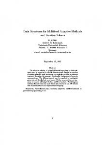
The set L i contain indices of the nodes that have no edges connecting them to the points in L i−1 . This procedure defines “concentric layers” of nodes defined by the graph Laplacian of the matrix A. Such an implementation of the breadth first search algorithm requires O (nJ + |E|) operations and is optimal if A is sparse. The next step consists in defining the coarse grid degrees of freedom, which is done in the way similar to the alternating construction used in 1d case. More precisely, we start by finding block tridiagonal form of A. We then remove all odd-numbered blocks and find block tridiagonal form of each connected component of each remaining even-numbered block. We repeat this process until only 1×1 and 2×2 blocks remain. The remaining evenly numbered “blocks” in the above procedure will be the coarse grid degrees of freedom. This procedure picks coarse nodes from each of the layers L i in such a way that coarse nodes are at least one node apart from each other in the graph defined by A, as demonstrated by Fig. 2.

3.4. Interpolation procedure To make the presentation of our multilevel scheme complete, we need to define the interpolation operators that appeared in Algorithm 3.2. Namely, we need to discuss the choice of the restriction and prolongation operators. To define an interpolatory connection for each degree of freedom, which does not appear on the coarse grid, we have to uniquely determine the points on coarse grid which will be used to interpolate the value of the fine grid degree of freedom.

203

Fast Multilevel Adaptive Binning Algorithm 100

90

coarse node #5

λ2=0.048857 λ =0.4467 8

coarse node #8

80 λ2=0.023757 λ4=0.74931 λ5=0.22693

70

coarse node #2 coarse node #4

60

λ =0.21561 λ28=0.38584

λ2=0.50422 λ =0.30401 λ46=0.19177

50

coarse node #6 40

coarse node #1 λ2=0.20162 λ3=0.63779

30

20

coarse node #3

coarse node #9 10

0

coarse node #7

0

10

20

30

40

50

60

70

80

90

100

Figure 2: A visualization of the grid oarsening part of the algorithm.

Figure 3: A s hemati view of the interpolation based on bary entri oordinates.

In Section 3.1 we introduced the following space decomposition: WJ =

ni J X X i=1 j=1

Wi, j =

J M

¯ i, W

i=1

n

i where Wi, j = span{ψij } for the canonical nodal basis {ψij } j=1 . Based on this basis, we can define an interpolator the following way. At every level, define a triangulation based on coarse grid nodes. Then for each fine grid point identify the unique triangle it belongs to in this triangulation and set

λi, j =



barycentric coordinate of a fine node i with respect to coarse node j .

Fig. 3 illustrates this definition.

(a)

(b)

Figure 4: (a) Support of the basis fun tions on the oarse level; (b) Corresponding nodal basis.

204

M. Emelianenko

¯i , · · · , ψ ¯ i ] T ∈ Rni ×k is constructed as follows: The interpolation matrix Q i = [ψ 1 n i

q j,ic = λ j,ic .

(3.3)

We further restrict the support of each basis function to the corresponding Voronoi cell as shown in Fig. 4. A simplified version of this procedure has been originally tested on parallelogram shaped domains [1]. Here we presented the generalized version of this algorithm which we are now ready to adapt to the context of binning.

4. Accelerated Multilevel CVT-based Adaptive Binning (MCVTBin) According to Gersho’s conjecture [26], for bounded and strictly positive densities, the size of the Voronoi intervals are inversely proportional to the one-third power of the underlying density at the midpoints of the intervals. This conjecture can be used to partition the domain into equal SNR regions. In a 2-dimensional problem, a CVT with a density function ρ = (S/N )2 , generates a tessellation with bins that asymptotically enclose a constant mass (constant SNR). The obtained VT is strongly dependent on the discrete nature of input data, which can pose problems with degenerate cells and pinned pixels. A way out proposed in [5] is to use a special initial configuration of generators produced by the so-called bin-accretion algorithm, which alleviates these issues as long as the underlying density is additive, i.e., (S/N )21+2 = (S/N )21 + (S/N )22 . The latter is true for all intensity maps subject to Poisson-distributed noise levels, which is the case under consideration. In order to adapt the multilevel scheme to the scope of discrete problems of this type, we adhere to the same strategy of producing a suitable starting configuration, as outlined below. Bin accretion starts by choosing the highest S/N pixel in the image. We then find centroid of the current bin and select the unbinned pixel closest to the centroid. We add the candidate to a chosen bin if: (a) the new pixel is adjacent to the current bin; (b) the morphology of the bin would remain below some threshold; (c) the S/N for this bin would get closer to (S/N ) T . The process is repeated until no new pixel can be added. Let ki denote the number of pixels in Vi . If the bin’s S/N computed as P ki Si (S/N )Vi = ÆPi=1 , ki 2 N i=1 i

is higher than some fraction of the target signal-to-noise ratio, e.g. 0.3(S/N ) T , we mark all the pixels in the bin as successfully binned, otherwise as unsuccessfully binned. We find mass centroid of all pixels already binned and start a new bin from an unbinned pixel closest to this centroid, then repeat until all pixels have been binned. Then we compute

Fast Multilevel Adaptive Binning Algorithm

205

centroid of each successful bin and reassign the unsuccessfully binned pixels to the closest of these centroids. It remains to recompute centroids of each bin obtained above and use them as input for the multilevel V (ν1 , 0)-cycle defined in Algorithm 3.1. This strategy serves as a first step of the main algorithm proposed in this study — Multilevel CVT-based Binning (MCVTBin) algorithm — which is outlined below.

Algorithm 4.1. MCVTBin algorithm. 1. Run bin accretion to generate initial configuration Z = {zi }ki=1 . 2. Perform a multilevel cycle V (ν1 , 0) described in Algorithm 3.1: For i = 1 : J (a) Use Algorithm 3.2 to define the partition Ti and coarse degrees of freedom. ni (b) Use formula (3.3) to compute nodal basis {ψij } j=1 . ˜ (c) Carry out ν1 smoothings H →min, find weights α jl and update the solution. Use CoarseGridSolve to obtain nearly exact solution on the coarsest level. 3. Repeat Step 2 until one of the convergence criteria is met.

Convergence criterion adopted in this implementation of the method is a superposition of the following conditions: (a) ||Zn − Zn−1 || < ε1 , (b) ||H˜(Zn ) − H˜e x ||/H˜0 < ε2 and (c) n > Ni t er , where Ni t er defines the maximum number of multilevel cycles. Exact numerical values of the energy H˜e x are not available in practice, but are used here to assess convergence and are obtained by running Lloyd iteration till saturation (a long time limit).

5. Numerical results Below we analyze the performance of the MCVTBin algorithm using a set of two largescale two-dimensional binning examples. The first one is a sample Integral-Field Spectroscopy (IFS) image provided by M. Cappellari (Oxford, UK), from the public repository at http://www-astro.physi s.ox.a .uk/ mx /idl/#binning. The data comes in a form of 3107 pixels, each with associated signal and noise values. Figs. 5(a,b) give a visualization of the original image and the result of the bin-accretion stage. The colormap is given by the SNR (signal-to-noise ratio), rescaled in the coarsened images to fit the range of remaining intensities for enhanced grid shape visualization. In Figs. 5(c,d) we compare the final binned image after 12 steps of the Lloyd algorithm (our implementation of the method of [5]), when the stopping criterion (a) was met, with that after 4 MCVTBin iterations, at which point criterion (b) was satisfied. The differences between the last two images are barely noticeable, which is to be expected due to the fact that both methods reach the same energy level at this point. It is clear that it takes MCVTBin less iterations than Lloyd to reach same accuracy level. The evolution of the energy and convergence estimates are given in Figs. 6 and 7. Convergence factor after n multilevel cycles is computed as ρ ≈ (||en||/||e0||)1/n , with the error en = H˜(Zn ) − H˜e x computed with respect to H˜e x estimate obtained as a limit of Lloyd iterations with the same number of generators.

206

M. Emelianenko 20

3000

20 400 15

15

350

2500 10

10

300 5

2000

5

0

1500

0

250 200

−5

−5

150

1000 −10 500

−15 −20 −20

−15

−10

−5

0

5

10

15

−10

100

−15

50

−20 −20

20

−15

−10

−5

0

(a)

5

10

15

20

(b)

20

20 400

15

400 15

350 10

350 10

300 5

250

0

200

−5

150

−10 −15 −20 −20

−15

−10

−5

0

(c)

5

10

15

20

300 5

250

0

200

−5

100

−10

50

−15

150 100 50

−20 −20

−15

−10

−5

0

5

10

15

20

(d)

Figure 5: (a) Original IFS image from SAURON data. (b) The image after bin a

retion. ( ) Result of Lloyd algorithm run until saturation. (d) Result of MCVTBin algorithm after 4 steps. 5

7.2

x 10

20

7 15

energy

6.8

10

5

6.6 0

6.4

−5

−10

6.2 −15

6

−20

0

2

4

6

8

10

12

−20

−15

−10

−5

0

5

10

15

20

25

Iteration number

Figure 6: (a) Convergen e of energies for Lloyd algorithm ( rosses) vs. MCVTBin (squares), for the IFS example. (b) Final Voronoi tessellation provided by the multilevel solution for the same data. Here we use the fact that since Lloyd method is globally convergent in the weak energy norm [1, 21], running Lloyd till stagnation yields a good approximation to the exact energy value. Reaching sufficiently low energy value is enough to ensure convergence of the algorithm in many practical applications, including the binning context considered here. MCVTBin does require more computational time per cycle, but this fact is offset by the evidence of uniform convergence provided in Fig. 7. Computational savings are associ-

Fast Multilevel Adaptive Binning Algorithm

207

Figure 7: Convergen e of the MCVTBin s heme for the IFS image: (a) the number of iterations required to rea h the a

ura y of ε = 10−6 does not grow, (b) omputational time required to rea h this a

ura y, ( ) onvergen e fa tor, omputed per multilevel y le. ated with the fact that convergence of MCVTBin does not slow down with the number of generators in contrast with the deterioration of the Lloyd method’s convergence. Fig. 6(b) shows the Voronoi tessellation obtained by the multilevel algorithm after 4 iterations. Although the computational savings that we obtained in this example are not dramatic due to the size limitations of the original dataset, by the nature of the algorithm the advantage of the MCVTBin method becomes much more visible as the size of the problem increases. The next example provides some further evidence of this fact. This time the set of tests comes from the analysis of the collective motions of magnetic moments within a slice of Cobalt. The data was obtained from the MAPS spectrometer at The Rutherford Appleton Laboratory (UK), courtesy of I. Bustinduy. It contains around 25k pixels with signal and noise values, given in the reciprocal space units, where u1 = [0.5Q h , 0, 0, 0] and u2 = [0.5Q h, −Q k , 0, 0]. Following standard notation, the indices h, k, l specify different crystal planes within the anisotropic structure of a crystalline solid, and the variables Q h, Q k , Q l are the corresponding changes of momentum in 3D space. Fig. 8 gives the original image and the result after the bin-accretion stage of the algorithm. Fig. 9 provides a visualization of the image at different coarsening levels of the multilevel algorithm. The original colormap represents the intensity given as a SNR (neutron counts), while The colormap in coarsened images has been rescaled to precisely match the full spectrum of representative intensities. The results of the benchmarking tests for this data are summarized in Fig. 10. As before, convergence factor is measured as the energy error reduction per cycle. MCVTBin produces same quality of binned image after a much smaller number of iterations (cf. [7, 9]) and, most importantly, preserves convergence factors when the number of pixels is increased. This means that the computational savings will increase even more as the size of the data grows. From the above analysis we also conclude that computational time required by the MCVTBin algorithm scales linearly with k (number of generators, specifying the size of the problem) for both examples. The method maintains uniform convergence with respect to the problem size similar to its 1-dimensional prototype developed in [1], which gives a

208 1.4

1.3

1.3

1.2

1.2

1.1

1.1 2

1.4

u

1

u

2

M. Emelianenko

1

0.9

0.9

0.8

0.8

0.7

0.7

0.6

0.6

0.5 −1

−0.8

−0.6

−0.4

−0.2

0.5 −1

0

−0.8

−0.6

u

u

−0.4

−0.2

0

1

1

Figure 8: Colle tive motions of magneti moments within obalt, where the spin dispersion volume is sli ed in the proje tion spa e dened by u1 = [0.5Q h, 0, 0, 0] and u2 = [0.5Q h, −Q k , 0, 0]: (left) Original experimental image of a magneti obalt system (25k pixels). (right) The image after bin a

retion (2136 pixels). Colormap represents neutron ounts.

1.4

1.4

1.4

1.3

1.3

1.3

1.2

1.2

1.2

1.1

1.1

1.1

1

1

1

0.9

0.9

0.9

0.8

0.8

0.8

0.7

0.7

0.7

0.6

0.6

0.5 −1

−0.8

−0.6

−0.4

(a)

−0.2

0

0.5 −1

0.6

−0.8

−0.6

(b)

−0.4

−0.2

0

0.5 −1

−0.8

−0.6

−0.4

−0.2

0

(c)

Figure 9: Comparison of grids at dierent oarse levels of the MCVTBin algorithm applied to the Cobaltsli e data from MAPS: (a) The mesh at the lowest level of the multilevel algorithm (29 oarse nodes of freedom), (b) The mesh at level 2 (122 degrees of freedom), ( ) The mesh at level 1 (512 degrees of freedom).

Figure 10: Convergen e of the MCVTBin s heme for the Cobalt image: (a) the number of iterations required to rea h the a

ura y of ε = 10−6 does not grow, (b) omputational time required to rea h this a

ura y, ( ) onvergen e fa tor, omputed per multilevel y le. Sin e the method onverges in 1 step when k = 2136, there is no onvergen e fa tor estimate available for this point in the rightmost graph. significant advantage compared to other iterative methods. Calculations were carried out on a 3GHz machine running a MATLAB implementation of the algorithm, which can be made significantly faster when coded in higher level programming language.

209

Fast Multilevel Adaptive Binning Algorithm

6. Conclusion and future work We have shown that the performance of CVT-based binning algorithms can be successfully optimized by means of multilevel accelerators such as the MCVTBin scheme introduced in this work. The extension of the multilevel quantization algorithm introduced in [1] to the two-dimensional case was made possible through barycentric coordinate based interpolation and maximal independent set coarsening procedures. Numerical evidence has been presented confirming the conjectured uniform convergence of the proposed scheme with respect to the problem size for two-dimensional examples with arbitrary densities, guaranteeing a significant speedup comparing with traditional methods. Care must be taken to produce an initial configuration allowing for guaranteed descent of the method into the area of fast convergence, which for example can be done through the widely known bin accretion technique. Note, however, that the bin accretion technique is important only when there is a danger of having on average very few data points inside each bin. This step can be completely avoided in case when the relative size of each Voronoi cell is large (e.g. ≈ 100 pixels per cell), with no toll on the convergence of the MCVTBin algorithm. The comprehensive analysis of convergence estimates for both regimes addressing the needs of different applications is currently underway. In addition, it might be possible to extend the method to non-Poissonian noise distributions and try choosing different interpolation and coarsening rules, which can potentially have big impact on the algorithm performance. In particular, such modifications can have a positive or negative effect on the size of the convergence region - a question that can be rigorously investigated via employing ideas from the algebraic multigrid theory. Rigorous convergence analysis and application of multilevel acceleration techniques to other image and signal analysis problems is a focus of a separate study and will be discussed in details in future publications. Acknowledgments The author wishes to thank anonymous referees for providing invaluable feedback that greatly improved the quality of the manuscript. The author is also indebted to Prof. Ludmil Zikatanov and Prof. Qiang Du of Penn State University for many fruitful discussions and help with the development of the original version of the multilevel algorithm, Zichao Di for assistance with running the code and Ibon Bustinduy for useful insights and for providing spectroscopy data that was used to benchmark the algorithm. The author was partially supported by the grants DMS 0405343 and DMR 0520425.

References [1] Q. Du and M. Emelianenko. Uniform convergence of a nonlinear energy-based multilevel quantization scheme via centroidal voronoi tessellations. SIAM J. Numer. Anal., 46:1483– 1502, 2008. [2] C. Wager, B. Coull, and N. Lange. Modelling spatial intensity for replicated inhomogeneous point patterns in brain imaging. Journal of Royal Statistical Society B, 66:429–446, 2004.

210

M. Emelianenko

[3] Q. Du, M. Emelianenko, Lee H.-C., and X. Wang. Ideal point distributions, best mode selections and optimal spatial partitions via centroidal voronoi tessellations. Proc. 2nd Intl. Symp. Voronoi Diagrams in Sciences and Engineering (VD2005), pages 325–333, 2005. [4] Q. Du, M. Gunzburger, L. Ju, and X. Wang. Centroidal voronoi tessellation algorithms for image compression, segmentation, and multichannel restoration. J. Math. Imaging Vis., 24(2):177–194, 2006. [5] M. Cappellari and Y. Copin. Adaptive spatial binning of integral-field spectroscopic data using voronoi tessellations. Mon. Not. R. Astrol. Soc., 342:345–354, 2003. [6] S. Diehl and T.S. Statler. Adaptive binning of x-ray data with weighted voronoi tessellations. Mon. Not. R. Astron. Soc., 368:497?10, 2006. [7] I. Bustinduy, F.J. Bermejo, T.G. Perring, and G. Bordel. Experimental neutron spectroscopy data visualization: Adaptive tessellation algorithm. Review of Scientific Instruments, 78:234509, 2007. [8] Q. Du and M. Emelianenko. Acceleration schemes for computing the centroidal voronoi tessellations. Numer. Linear Algebra Appl., 13:173–192, 2006. [9] I. Bustinduy, F.J. Bermejo, T.G. Perring, and G. Bordel. A multiresolution data visualization tool for applications in neutron time-of-flight spectroscopy. Nuclear Inst. and Methods in Physics Research, A., 546:498–508, 2005. [10] Q. Du, V. Faber, and M. Gunzburger. Centroidal voronoi tessellations: applications and algorithms. SIAM Review, 41:637–676, 1999. [11] S. Lloyd. Least square quantization in pcm. IEEE Transactions on Information Theory, 28:129– 137, 1982. [12] R. Gray and D. Neuhoff. Quantization. IEEE Transactions on Information Theory, 44:2325– 2383, 1998. [13] L. Ju, M. Gunzburger, and Q. Du. Meshfree, probabilistic determination of points, support spheres, and connectivities for meshless computing. Computational Methods in Applied Mechanics and Engineering, 191:1349–1366, 2002. [14] Y. Linde, A. Buzo, and R. Gray. An algorithms for vector quantizer design. IEEE Transactions on Communications, 28:84–95, 1980. [15] J. MacQueen. Some methods for classification and analysis of multivariate observations. Proc. 5th Berkeley Symp. Math. Stat. Prob., I, Edited by L. LeCam & J. Neyman, pages 281– 297, 1967. [16] A. Trushkin. On the design of an optimal quantizer. IEEE Transactions on Information Theory, 39:1180–1194, 1993. [17] Q. Du and M. Gunzburger. Grid generation and optimization based on centroidal voronoi tessellations. Applied Mathematics and Computation, 133:591–607, 2002. [18] J. Cortes, S. Martinez, T. Karata, and F. Bullo. Coverage control for mobile sensing networks. IEEE Transactions on Robotics and Automation, 20:243–255, 2004. [19] L. Ju, Q. Du, and M. Gunzburger. Probabilistic methods for centroidal voronoi tessellations and their parallel implementations. Parallel Computing, 28:1477–1500, 2002. [20] Q. Du, M. Emelianenko, and L. Ju. Convergence properties of the lloyd algorithm for computing the centroidal voronoi tessellations. SIAM J. Numer. Anal., 44:102–119, 2006. [21] M. Emelianenko, L. Ju, and A. Rand. Weak global convergence of the lloyd method for computing centroidal voronoi tessellations in r d . SIAM J. Numer. Anal., 46:1423–1441, 2008. [22] Koren Y., Yavneh I., and A. Spira. A multigrid approach to the scalar quantization problem. IEEE Transactions on Information Theory, 51(8):2993–2998, 2005. [23] Koren Y. and Yavneh I. Adaptive multiscale redistribution for vector quantization. SIAM Journal on Scientific Computing, 27(5):1573–1593, 2006.

Fast Multilevel Adaptive Binning Algorithm

211

[24] Q. Chang and Z. Huang. Efficient algebraic multigrid algorithms and their convergence. SIAM Journal on Scientific Computing, 24:597–618, 2002. [25] X. Tai and J. Xu. Global convergence of subspace correction methods for some convex optimization problems. Mathematics of Computation, 71:105–124, 2002. [26] A. Gersho. Asymptotically optimal block quantization. IEEE Transactions on Information Theory, 25:373–380, 1979.