close to Matlab. Figure 1 Dog with bounding box (from ImageNet synset). Page 2. Figure 2 Dog HOG visualization. Figure 3
Fast Object Detection with Whiten Hog Feature and its implementation in OpenCV For course 91.550 Object Recognition 2013 Fall Semester Hualiang Xu
[email protected] Abstract Traditional object detection employs HOG feature with Support Vector Machine (SVM), which works but with limitations such as training cost on each cluster. In this paper, we are going to introduce LDA that refines the feature by removing the correlation of the feature dimensions. We implemented the learning and detection in OpenCV that makes the code portable to all platforms.
1. Introduction HOG (Histogram of Gradient) feature was first introduced by Navneet Dala and Bill Triggs in 2005, for the task of pedestrian detection. It is based on well-normalized local histograms of image gradient orientations in a dense grid. Figure 2 shows the HOG representation of the source figure 1. They gain better results by an order of magnitude comparing to the best technique at the time. More recent research like Deformable Part Model (DPM) builds up on that also achieve great success. SVM (Support Vector Machine) is a nonprobabilistic binary linear classifier that separates two classes by maximizing the inbetween margin. Data points that are within the margin are penalized in the cost function.
However, SVM is not the only linear classifier. Fisher’s LDA method tries to maximize the in-between class variance over the in-class variance. Bharath et al put the LDA theory to the HOG features, up on which they generated the whiten HOG feature, called WHO. We used OpenCV in the implementation and evaluation. OpenCV is open source computer vision library released under BSD license. It provides features/APIs that is close to Matlab.
Figure 1 Dog with bounding box (from ImageNet synset)
compressed. Mathematically, this is done either by Eigen vector/value computation or Singular Value Decomposition (SVD). The Eigen vector exhibits orthogonal property, which we use as the rotated coordinate. The Eigen value exhibits the scatter-bility on each axis.
Figure 2 Dog HOG visualization
PCA and LDA differ in that PCA is to reduce the feature to address the curse of high dimensionality in computation cost, while LDA is to increase the separability.
Figure 4 LDA
3. Whiten Hog Feature Figure 3 Dog Patch HOG visualization
2. LDA The Linear Discriminative Analysis is to find the transform spec, such that in such space, the in-between class scatter (Sb) is high, and the in-class scatter (Sw) is low, and we expect the ratio of Sb/Sw to be high. See figure 4. Principle Component Analysis (PCA) is a similar method that reduces the feature dimensionality. The n-dimension coordinate is rotated such that the scatter-bility on each axis is sorted. And we throw away some of the axis that gives less scatter-bility. We say the feature dimensionality is reduced, or in other words feature is
In out implementation, we define the filter window to be 10 by 11 cells, each of which takes 8 by 8 pixels. On each cell, we compute 32 dimension HOG feature. The total dimensionality is 3520. So we have the covariance matrix ∑ with dimensionality 3520 by 3520. The covariance matrix ∑ for each class is assumed to be equal to the background (sum of all the classes). We assume each class follows Gaussian distribution: P(x|y) = N(x; uy, ∑) A LDA model can be represented as: w = ∑-1(u1 – u0)
where u0 is the mean of the background (see figure 5 as its visualization), u1 is the mean of class 1. Intuitively, we are shifting the feature such that it is zero-meaned (see figure 6), and by dividing to the covariance matrix, we are removing the correlation of each feature dimension (see figure 7). Bharath et al call this process as “whitening”, and the feature of the whitened HOG as WHO. And the classifier as: w * x, which is equivalent to P(x|1) > P(x|0).
Figure 6 Dog zero-mean hog visualization
Figure 5 Background HOG
Figure 7 Dog WHO visualization
4. Data Set We used ImageNet synset (with labeled bounding box) for training and testing. Insitu image will be used for adaption in the
future work. We expect the detection accuracy to be improved with model adaption. ImangeNet offers 14 million images and over 21k synsets, each of which with hundreds of images. In our experiment, we used two sets of the sysnets: bear mug and dog. The labeled bounding boxes are stored in a separate xml file. Inside the computer filesystem, a description file helps matching the name of the category and its synset name. By type in the category name to learn, the computer looks up the description file and outputs the name of the synset. After that, the computer downloads the bounding box and the image sets, unzip to a designated folder for further study.
Owing to the marginalization not considered in the detection, the detection accuracy is not good. This is natural that the real object is not in the learned ratio in its height and width, pyramid in combined ratio on x and y direction should improve the detection result. Adaption to the in-situ model should also improve the accuracy. Initial accuracy on dog detection is 11.33% and beer mug is 36.64%. By building up the pyramid on both x and y direction, dog and beer mug detection reach 18.72% and 48.8% respectively. The tradeoff here is the detection speed slows down. A couple of good detections are listed below:
The previously downloaded bounding box and image sets are keep on the computer for future use. In-situ model is not included in this writeup, but here is a few words. In case of a robot, it takes in-situ images for training. This is helpful in that of the model shifting. We are going to adapt the in-situ model by: f(x) = max(fonline(x), fofline(x))
5. Evaluation By evaluation, we separate the imangenet synset into 70% training and 30% testing. Bounding box with 50% overlap on the label and detection is treated as a good detection. For each input image, we take its pyramid HOG features. Under each layer of the pyramid, we run the convolution to the learned classifier w.
Figure 8 Dog good detection (Green – label, Red – detection)
6. Discussion and Future Work Although the detection didn’t achieve the good accuracy, it proved the LDA learning and detection flow in OpenCV implementation. Marginalization might improve the accuracy significantly.
Figure 9 Beer mug good detection (Green – label, Red – detection)
Other than that, DPM and FFT can improve the accuracy and detection speed respectively. Model adaption to in-situ parameters is another direction.
And here is the bad detection:
References [1]. Navneet Dalal and Bill Triggs: Histograms of Oriented Gradients for Human Detection
[2]. Bharath Hariharan, Jitendra Malik, and Deva Ramanan: Discriminative Decorrelation for Clustering and Classification
[3]. Felzenszwalb, P., Girshick, R., McAllester, D., Ramanan, D.: Object detection with discriminatively trained partbased models
[3]. OpenCV Online documentation: http://docs.opencv.org
[4]. Max Welling: Fisher Linear Discriminant Analysis Figure 10 beer mug bad detection (Green – label, Red – detection)
In the case of figure 10 bad detection, the red box gain high score in that it looks like a mug. We don’t gain the correct detection owing to the window is not scaled in correct ratio in x/y direction.
[5]. Principal Component Analysis: http://www.stat.cmu.edu/~cshalizi/490/pc a/pca-handout.pdf