synchronization, frequency synthesis, FM demodulation, clock and data recovery, etc. Despite their application in circuits over decades, modern PLL design still ...
1
Fast PLL Simulation Using Nonlinear VCO Macromodels for Accurate Prediction of Jitter and Cycle-Slipping due to Loop Non-idealities and Supply Noise Xiaolue Lai, Yayun Wan and Jaijeet Roychowdhury Department of Electrical and Computer Engineering University of Minnesota Email: {laixl, yayun, jr}@ece.umn.edu
Abstract— Phase-locked loops (PLLs) are widely used in electronic systems. As PLL malfunction is one of the most important factors in re-fabs of SoCs, fast simulation of PLLs to capture non-ideal behavior accurately is an immediate, pressing need in the semiconductor design industry. In this paper, we present a nonlinear macromodel based PLL simulation technique that is considerably more accurate than prior linear PLL simulation techniques. Our method is able to accurately capture transient behavior and faithfully estimate timing jitter in noisy PLLs. We demonstrate the proposed technique on ring and LC voltagecontrolled oscillator (VCO) based PLLs, and compare results against linear PLL macromodels and full SPICE-level simulation. We show that, unlike prior linear macromodel based approaches, the proposed nonlinear technique captures the dynamics of complex phenomena such as locking, cycle slipping and power supply noise induced PLL jitter, replicating qualitative features from full SPICE simulations accurately while providing speedups of over two orders of magnitude.
I. I NTRODUCTION PLLs [14] are extensively used in all analog and digital systems. Their uses include clock generation, signal conditioning and synchronization, frequency synthesis, FM demodulation, clock and data recovery, etc. Despite their application in circuits over decades, modern PLL design still presents significant challenges. In actual fabrications and real designs, PLLs often do not function as they are ideally supposed to, due to second-order effects such as non-ideal filters, interference from power supply lines, loop stability issues, etc.. Indeed, in modern RF and mixed-signal designs (especially for SoCs) functional degradation of PLLs is a major cause of overall system malfunction, often resulting in many design and fabrication re-spins. Costs of such re-fabs can run into the millions of dollars and significantly delay product time-to-market. As a result, accurate simulation of PLLs is of great practical importance. Direct timedomain simulation of PLLs at the level of SPICE circuits is typically impractical because of its great inefficiency. PLL transients can last hundreds of thousands of cycles, with each cycle requiring hundreds of small timesteps for accurate simulation of the embedded voltage-controlled oscillator (VCO). Furthermore, extracting phase or frequency information, one of the chief metrics of PLL performance, from time-domain voltage/current waveforms is often difficult and inaccurate. To alleviate the inefficiency of simulating PLLs at the SPICE level, a popular approach towards approximate PLL simulation involves the use of phase domain macromodels (e.g., [8]). In this approach, each building block of a PLL (such as the VCO, the phase/frequency detector, and the low-pass filter) is represented approximately using small, simple macromodels, and the system of macromodels simulated. Furthermore, in contrast to SPICE-level circuits which use voltage/current domain device models, the PLL block macromodels used are typically in the phase domain. For example, in traditional approaches, the VCO is represented as a simple linear integrator that converts input voltages to output phases; similar simple macromodels of other blocks are also employed. The use of such macromodels can lead to dramatic speedups (of many orders of magnitude over the SPICE level); however, such speedups are obtained at the expense of accuracy. As we show in this paper, the use of linear macromodels can lead to qualitatively incorrect prediction of important PLL phenomena.
Linear PLL block macromodels, while appropriate for simple, locked PLLs in near-ideal operation (e.g., the low-pass filter (LPF) rejects high frequencies well, there is no interference from power supply/ground lines, etc.), can be seriously inadequate for predicting the complex non-ideal phenomena that are typically responsible for performance degradation in today’s industrial PLLs. For example, high-bandwidth PLLs (e.g., [13], [10]), popular in read channel and clock recovery applications for their fast tracking properties, are difficult to simulate accurately using linear macromodels because the high-frequency components transmitted from the phase/frequency detector to the VCO excite nonlinear mechanisms critical for capture/lock and cycle slipping. Such mechanisms often result in changes to the static phase offset of the PLL in lock; these changes in static offset consume additional phase budgets for a stable lock and affect the likelihood of cycle slipping (e.g., [7]). Linear methods do not take these non-idealities into consideration, thus resulting in incorrect predictions. Moreover, charge pump PLLs (e.g., [1], [12]), widely used for frequency synthesis, usually feature a feed-forward channel bypassing the low-pass filter to ensure loop stability. The high-frequency components transmitted through these feed-forward paths again invalidate linear macromodels. Furthermore, linear VCO macromodels typically have difficulty accounting for supply- or substrate-interference-induced PLL phase jitter (e.g., [8], [11]). In the deep-submicron technologies in predominant use today, interference-induced jitter has grown to be a primary cause of PLL performance degradation. Since jitter is mainly created by direct interference to the VCO, the (ideally slow) loop dynamics of the PLL is unable to eliminate it appreciably; again, fast nonlinear mechanisms are excited which linear macromodels [6], [16], [2], [15], [9], [5] are ill-suited to cope with [3]. To address the above macromodel-based simulation accuracy issues, while still providing large speedups over full SPICE-level simulation, we present a macromodel-based PLL simulation technique that employs automatically extracted, nonlinear, VCO phase domain macromodels [3]. In our method, the phase deviation of the VCO is captured using a single, scalar nonlinear differential equation with as many inputs as desired. The inputs include (but are not limited to) not only the control input of the VCO, but also interference and noise sources from the power supply, ground, substrate, etc... The key advantage of this technique is that it considers nonidealities and nonlinearities in the PLL loop. As a result, the transient behavior of PLLs can be simulated far more accurately than with linear macromodels: phase noise in the PLL’s reference signal, high-frequency components from the phase/frequency detector, power supply, ground and substrate interference are all accounted for correctly. To demonstrate the capabilities of the proposed technique, we apply it to estimating static phase offset, simulating step response, cycle slipping and supply-interference effects of a high-bandwidth PLL structure. We provide comparison against simulations with linear macromodels and full simulation, demonstrating that the new technique provides accuracies essentially equivalent to full SPICElevel simulation, but with speedups of over two orders of magnitude. Furthermore, we demonstrate how the same simulations, but using linear macromodels, can completely fail to predict important phenomena such as cycle slips and supply-induced jitter. The remainder of the paper is organized as follows. In Section II,
2
we briefly review previous linear models and identify their shortcomings for our problem. In Section III, we review the nonlinear oscillator macromodel for PLL timing jitter estimation and derive the nonlinear PLL macromodel in ODE form. In Section IV, we present simulation results on both LC and ring VCO based PLLs, and compare the results with linear models and full SPICE-level simulation. II. R EVIEW OF L INEAR P HASE M ACROMODELS The block diagram of a PLL is shown in Figure 1. It consists of a phase/frequency detector (PFD), a low-pass filter (LPF), a voltage-controlled oscillator (VCO) and a frequency divider (FD). The FD is usually used when the PLL is a frequency synthesizer. The PFD compares the phase difference between the reference frequency fre f and the feedback frequency f f b and produces a voltage which corresponds to the phase difference between two signals. Since the output of the PFD has high frequency AC components, an LPF is applied to filter out these AC components and provides a DC voltage to control the VCO. The PLL is a feed-back loop, which means that when it is in lock, the feedback frequency f f b is forced to be identical to the reference frequency f re f . Given an input frequency f re f , the frequency at the output of the PLL is f out = N fre f . f re f
- PFD - LPF - VCO
f out
-
f fb
FD � ÷N Fig. 1.
Functional block diagram of a PLL.
It is well known that direct simulation of PLLs in time domain is very expensive since the PLL requires many periods of the VCO to reach the steady-state. This is especially true when we simulate frequency synthesizers with large multiplication factors. To simulate the phase of the PLL accurately, the simulator has to use many timesteps for every cycle of the VCO, and the locking process often takes hundreds or thousands of cycles at the reference input. Hence, full simulation of PLLs at SPICE-level consumes a lot of computational resources. Simulating the PLL directly in phase can significantly saves computational time, because the VCO is treated as a phase generator and no oscillator is involved in the simulation. A linear phase-domain model of a PLL is shown in Figure 2. f re f
- l - Kpd f (∆φ ) - H(S) 6 f fb � 1
Kvco S
f out
-
N
Fig. 2.
Linear phase-domain model of a PLL.
In this phase domain macromodel, the PFD is modeled as Kpd f (∆φ ), where K pd is the gain of the PFD and f (∆φ ) is the transformation function between the phase difference and the output voltage of the PFD, which depends on the type of the PFDs. For example, if the PFD is a mixer/multiplier, the transformation function can be defined as f (∆φ ) = sin(∆φ ); if the PFD is a XOR phase detector, the transformation function is f (∆φ ) = ∆2πφ , if the LPF is ideal and can filter all ACs out. The VCO is an oscillator that converts its input voltage to an output frequency. The relationship between input voltage and output frequency is considered to be linear time-invariant (LTI) and can be expressed as fout (t) = KVCO vc (t) + f0 , (1)
where f0 is the VCO’s central frequency, KVCO is the gain of the VCO and vc (t) is the control voltage from the LPF. The output phase of the VCO can then be given by
φout (t) = 2π f0 t + 2π
Z
KVCO vc (t)dt.
(2)
this linear model is very suitable for studying the phase deviation of the pll under small perturbations when the PLL is in lock, as long as we only concern how the perturbation affects the phase of the PLL. However, it suffers from some drawbacks. Since the VCO is treated as a LTI system and the high frequency components from the PFD is ignored, the model is unable to capture nonlinear dynamics in the loop which affects the behavior of PLLs. In addition, this model can not predict the phase deviation caused by power supply and substrate noise since the linear VCO model is unable to translate noise currents/voltages into phase deviation. III. PLL SIMULATION USING NONLINEAR VCO PHASE MACROMODELS
To solve the above problems in linear macromodels, we develop a nonlinear PLL macromodel, which simulates the behavior of PLLs more accurately. Our nonlinear phase-domain macromodel is closely related to recent oscillator phase noise and jitter theories [3], and can precisely capture the transient behavior of PLLs and approximate the timing jitter of PLLs in the presence of perturbations, both random and deterministic. A. The Nonlinear Oscillator Phase Model In this section, we provide a brief review of the nonlinear phase model in [3], which we adapt in this work in order to build the nonlinear PLL phase-domain macromodel. A general oscillator can be expressed as x˙ = f (x) + b(t)
(3)
where b(t) are perturbations to the free running oscillator. We can assume the solution of the perturbed oscillator is x p (t) = xs (t + α (t)) + y(t),
(4)
where xs (t) is the steady-state solution of the unperturbed oscillator. Hence, the effect of the perturbations b(t) to the oscillator is partitioned into two parts: the phase shift α (t) to the unperturbed oscillator and the amplitude deviation y(t). The phase shift α (t) due to the perturbation is governed by the nonlinear differential equation
α˙ (t) = V1T (t + α (t)) · b(t)
(5)
where V1 (t) is the perturbation projection vector (PPV) which has the same period as the oscillator. The phase shift α (t) due to perturbations in the nonlinear phase model has the unit of time. Phase shift in radians can be obtained by multiplying α (t) by the free running oscillation frequency ω0 . The PPV is a vector of waveforms, each of them represents the oscillator’s phase sensitivity to noise injected to the corresponding circuit node on the oscillator. The PPV can be extracted from the SPICE-level description of oscillator circuits by numerical methods effectively [4], [3] and applied to study the oscillator’s behavior under perturbations. B. Nonlinear Phase-domain Macromodel of PLL Figure 3 depicts the block diagram of our nonlinear PLL macromodel. We use the nonlinear VCO macromodel proposed in [3] as replacements for the linear ones that have so far been used. In this macromodel, the VCO is no longer a simple linear integration component, instead, it is modeled as an oscillator perturbed by multiple injection signals: one is the control signal from the LPF, others are perturbation signals injected into circuit nodes on the VCO.
3
- m - Kpd f (φ1 , φ2 ) - x˙ = Ax + b -α˙ (t) = v1 (t + α (t))b(t) 6 f
fb
1/N
Fig. 3.
fout
-
for capturing injection-locking-related phenomena on a ring oscillator based PLL. Our method can predict the phase deviations of the PLL correctly, while the linear methods fail in this case, providing totally wrong prediction.
�
A. Building the PLL macromodel
Nonlinear phase-domain model of a PLL.
The differential equation for the phase deviation of the VCO can be of the form:
α˙ (t) = Vvc (t + α (t))vc (t) +VnT (t + α (t))n(t),
(6)
where vc (t) is the control voltage from the LPF, Vvc (t) is the PPV of the VCO control node, Vn (t) is a vector of PPV waveforms representing the VCO’s phase sensitivity to the noise injected into the corresponding circuit nodes and n(t) is the noise current/voltage applied to the VCO. The major differences between our nonlinear macromodel and traditional linear model are the inclusion of the phase shift α (t) inside the perturbation projection vector Vn (t) and the gain of the VCO Vvc (t) is no longer a constant. Since (6) gives the phase shift of the PLL under control voltage and perturbations in time. The total phase of the VCO in radians can be expressed as
φout (t) = ω0 (t + α (t)),
(7)
where ω0 is the VCO’s free-running frequency. The model of the PFD in our macromodel is slightly different than that of the linear macromodel. We retain the high frequency components to ensure we can capture the dynamics in the loop precisely. The PFD is modeled as K pd f (φ1 , φ2 ), where K pd is the gain of the PFD and f (φ1 , φ2 ) is a function that takes two phases as inputs and output a voltage. If we use a mixer/multiplier as the PFD, the function can be defined as f (φ1 , φ2 )
= =
sin(φ1 − φ2 ) + sin(φ1 + φ2 ) sin(φre f (t) − ω0 (t + α (t)) + sin(φre f (t) + ω0 (t + α (t)).
(8)
where φre f (t) is the phase of the reference signal, ω0 is the VCO’s free-running frequency, and α (t) is the VCO’s phase shift computed by (6). If we formulate the transfer function of the LPF H(S) in its ODE form and combine it with our nonlinear VCO phase model, we can reduce the original PLL system to an ODE system with a much smaller system size. Since the phase of the PLL is calculated directly in this macromodel, we can use much larger timesteps to simulate the PLL, resulting in great speedup. Our nonlinear model has taken the nonidealities in the PLL loop into consideration, thus, it captures the nonlinear dynamics in the transient behavior of PLLs much better than traditional linear models. In addition, our VCO macromodel is a noise model, which accurately predicts the phase shift caused by power supply and substrate noise. Hence, our macromodel has the capability to correctly simulate the behavior of PLLs under the influence of perturbations. IV. E XPERIMENTAL R ESULTS In this section, the nonlinear method discussed in Section III is applied to predict the pull-in process, cycle slipping and injection locking in PLLs. We first build the PLL macromodels using the method in Section III and derive the reduced ODE equations for our test circuits. Using the LC oscillator based PLL, We calculate static phase offset, simulate the pull-in process under different reference frequencies, and predict the cycle slipping under different initial phase errors. Our method provides good matches to full SPICE-level simulation, with great speedup. We also demonstrate the ability of our method
The PLL circuit we use in our experiment is shown in Figure 4. The circuit has a mixer as the phase detector and a low-pass filter with high bandwidth, with which we can simulate the non-idealities in the PLL. The system size of this simple PLL circuit is 14. In this circuit, the center frequency of the VCO is designed to be f 0 =100MHz and the RC pole is designed to leak appropriate AC components (0.2v in amplitude) to the VCO. Using the method we discussed in Section III, we can reduce the system size to 3.
− +
Vref+
Vctrl
Vref+
L
C
R
i=f(v)
Vref− Vvco+ Vvco−
Fig. 4.
An LC oscillator based PLL.
1) PFD Model: The output of the PFD is defined by (8), the only parameter we need to identity here is the gain of the PFD k pd . We run full circuit simulation on this PFD with different input phases and plot the relationship between the phase difference on two inputs and the output voltage of the PFD as Figure 5. It is clear from the figure 0.5 0.4 0.3
PFD Output Voltage (v)
fre f
0.2
y=−0.16x
0.1 0 −0.1 −0.2 −0.3 −0.4 −0.5 −1
−0.8
−0.6
−0.4
−0.2
0
0.2
0.4
0.6
0.8
1
sin(∆φ)
Fig. 5.
Gain of phase detector.
that the gain of the PFD has a very good linearity in its working range. In this PLL circuit, K pd of the phase detector has the value of −0.16. 2) LPF Macromodel: The transfer function of the Low Pass Filter can be derived from the circuit diagram directly. It has the form of H(s) =
3 + 2τ s , (1 + τ s)2
(9)
where, τ is the RC pole of the LPF. Using the companion form method, we can rebuild the ODE equations of the LPF as ( x˙1 (t) = x2 (t) (10) 2 x˙2 (t) = − x1τ(t) 2 − τ x2 (t) + b(t),
4 0.1
where b(t) is the output of the phase detector. The output of the LPF has the form of (11) y(t) = 3x1 (t) + 2τ x2 (t).
Static Phase Offset (rad)
0
3) Nonlinear VCO Macromodel: The nonlinear VCO phase model can be calculated by numerical methods [3], [4] directly from its SPICE-level circuit equations. In this experiment, we use the time-domain method introduced in [3] to calculate the PPV of the oscillator, as shown in Figure 6.
−0.1 Full Simulation Nonlinear MacroModel Linear Model
−0.2 −0.3 −0.4
0.1
−0.5 0
0
Fig. 7.
PPV(s/v)
−0.1
0.5
1
1.5 time (T)
2
2.5
3
The static phase offset of PLL when f re f = f 0 .
−0.2
−0.3
−0.4
Fig. 6.
2
4
Time (s)
6
8
10
−9
x 10
The PPV of the control node of the LC VCO.
It can be clearly seen that the VCO is not a LTI system, as the phase sensitivity of the control node is very dependent of when the control signal is applied. The linear VCO model uses the average of the PPV waveform as KVCO , so it can not capture the dynamics of the PLL correctly. 4) PLL Macromodel: Combining the LPF model, the PFD model and the VCO model together, we get the reduced PLL macromodel, which can be expressed as T α˙ (t) = Vvc (t + α (t))(3x1 (t) + 2τ x2 (t)) +Vn (t)n(t) x˙1 (t) = x2 (t) (12) x˙ (t) = − x1 (t) − 2 x (t) + K f (φ , φ ), 2 re f pd fb τ 2 τ2 where f (φre f , φ f b ) is defined by (8) and n(t) is the noise signal applied to the VCO. This reduced system can be simulated by any transient solvers, with great speedup. Using full SPICE-level simulation, the runtime in Matlab is about 150 minutes for a simulation time of 600 cycles. However, it takes only 1 minutes to simulate the same number of cycles using the nonlinear PLL phase macromodel – an approximately 150 times speedup.
B. Transient Simulation Using the nonlinear macromodel, we simulate the transient behavior of the PLL and compare the results with full simulation and linear models. We simulate the static phase offset, step response and cycle slipping of the PLL, the results show that our nonlinear macromodel matches the full SPICE-level simulation well, providing more precise simulation than linear models. 1) Static Phase Offset: One desirable property of PLLs is that the clock edge of the reference signal and the feedback from VCO can be brought into very close alignment. The average difference between the phases of these two signals when the PLL is in lock is called the static phase offset. Even though the circuit we use in this experiment is a first-order PLL, the phase difference between the reference signal and the feedback signal is suppose to be zero if we apply a reference signal with frequency that is identical to the VCO’s free running frequency, since the VCO requires a zero control input. However, if the LPF is not perfect and the AC signals from the PFD are leaked to the VCO, they may impact the static phase offset of the PLL via an injection-locking-like effect.
Figure 7 depict the static phase offset of the PLL when we apply a reference that has the same frequency as the VCO’s free-running frequency. We simulate the PLL to steady-state and plot the phase difference between the reference signal and the feedback signal. Since the LPF is not perfect, it cannot filter out the high-frequency AC components from the PFD completely; both full simulation and our nonlinear macromodel show the PLL has a static phase offset of about 0.43 radians. However, the linear model cannot capture this correctly, reporting a static phase offset of 0. 2) Step Response Simulation: We simulate the step response of the PLL under different reference frequencies and plot the results in Figure 8. Figure 8(a) depicts the step response of the PLL using full simulation, the linear phase model and the nonlinear macromodel when the reference frequency is 1.07 f 0 . With this reference signal, both linear and nonlinear macromodels track the reference frequency well, although, as expected, the nonlinear model provides a more accurate simulation than the linear one. When we increase the reference frequency to 1.074 f 0 , the linear phase macromodel cannot track the reference correctly, as shown in Figure 8(b). In contrast, our nonlinear macromodel can track the reference signal with full precision. Finally, we increase the reference frequency to 1.083 f 0 , which is beyond the pull-in range of the PLL circuit, so the PLL cannot lock. Even in this case, the transient behavior predicted by our macromodel matches full simulation very well. 3) Cycle Slipping Simulation: The PLL is a phase estimator which has multiple stable solutions with an interval of 2π . Once a PLL enters its locking mode, it tends to maintain a steady state condition where the phase error lies between its slip boundaries. Cycle slipping occurs when the phase error of the PLL accumulates to such a critical point that its feedback loop is unable to correct the error, resulting in a phase jump or ’slip’ from one locked steady-state point to another. Cycle slipping degrades the frequency estimation capability of PLLs and produces isolated bursts of large phase noise. To study cycle slipping in the PLL, we inject a sinusoid to the VCO to pull the PLL away from its steady-state and provide an initial phase error. The PLL may jump to another steady point, or return to the original one, depending on the extent of error and the dynamics of the loop. Investigating cycle slipping for different initial phase errors, we plot the results in Figure 9. We first provide a reference frequency fre f = 1.07 f0 and simulate the PLL to its steady-state. Then we inject a sinusoid perturbation with amplitude of 5mA to the VCO; the duration of the injected signal is 10 periods. This perturbation gives an initial phase shift of 1.2 in radians. The full simulation demonstrates the presence of cycle slipping in the PLL, as shown in Figure 9(a). Both nonlinear and linear macromodels predict this qualitative phenomenon correctly, with the nonlinear macromodel matching the full simulation better than the linear one. Next, we reduce the injection amplitude to 3mA, and run the simulation again. For this excitation, the initial phase offset due to the perturbation is about 0.6 radians, and the PLL can return to its original steady state
5
1.07
0
1.06 VCO Frequency (GHz)
−1 Cycle Slipping Phase Change (rad)
1.05 1.04 1.03 1.02 1.01 Full Simulation Linear Model Nonlinear MacroModel
1 0.99 0
5
time (T)
10
15
−2 −3 −4 −5 −6 −7 0
(a) f re f = 1.07 f 0
Full Simulation Linear Model Nonlinear MacroModel 10
20
30 time (T)
40
50
60
(a) Noise amplitude is 5mA
VCO Frequency (GHz)
1.1 1
1.05
0 −1 Phase shift (rad)
1
Full Simulation Linear Model Nonlinear MacroModel
0.95
0
50
100
150
−2 −3 −4
Full simulation Nonlinear macromodel Linear macromodel
−5
200
−6 −7 0
(b) f re f = 1.074 f 0
50
100
Time (T)
150
(b) Noise amplitude is 3mA 1.1
Fig. 9.
VCO Frequency (GHz)
1.05
Cycle slipping in the PLL under different noise amplitudes.
1 Vdd
0.95 0.9 0.85 0.8 0
Full Simulation Linear Model Nonlinear MacroModel 50
100
150
1
2
3
200
time (T)
(c) f re f = 1.083 f 0 Fig. 8.
Fig. 10.
A ring oscillator VCO.
The step response of the PLL under different reference frequencies. 5000
0.17
C. Simulation of Injection Locking Effects in PLLs We demonstrate the ability of the nonlinear macromodel to capture injection-locking-type behaviours in PLLs, using a ring oscillator VCO. We use the ring oscillator VCO shown in Figure 10 to replace the LC one in Figure 4. The PPV of the ring oscillator VCO is shown in Figure 11. To predict injection locking effects in the PLL, we first apply a reference frequency of 1.06 f 0 . After the PLL is in lock, we start to inject periodic perturbations to the node 1 of the VCO, as shown in Figure 10, and observe the phase shift of the PLL.
PPV (t/A)
0.16 PPV(s/v)
phase error. The nonlinear macromodel provides a close match to full simulation for this case; however, the linear model is unable to, predicting completely erroneous behaviour.
0
0.15
0.14 0
100
200 Time (s)
300
(a) PPV of the control node
Fig. 11.
400
−5000 0
0.5 Time (s)
1
(b) PPV of the stage-one output node
PPV of the ring oscillator VCO.
−8
x 10
6
1
5 0 −5 Phase shift (rad)
Phase shift (rad)
0.5
−10
0
−15 −20
−0.5
−25 −30
−1 0
100
200 300 Time (T)
400
−35 0
500
(a) Full simulation (injection amplitude = 0.01mA)
100
200 300 Time (T)
400
500
(b) Full simulation (injection amplitude = 0.02mA)
VCO macromodel that is extracted via algorithm from a SPICElevel circuit description. The macromodel correctly accounts for the nonlinear impact of a multiplicity of control and interference inputs to the VCO. Using the nonlinear phase domain macromodel, we are able to simulate a variety of PLL transient responses speedily at SPICE-level accuracies. Applications of our technique include predicting cycle slipping, high-frequency feed-through effects and injection-locking-like interference effects leading to jitter. Thus our technique is particularly relevant to modern PLL architectures with non-traditional modes of operation. We have also demonstrated how prior linear macromodels for PLL simulation can suffer from serious shortcomings in their predictive ability in these cases. R EFERENCES
5
1
0 −5 Phase shift (rad)
Phase shift (rad)
0.5
−10 −15
0
−20 −25
−0.5
−30 −1 0
100
200 300 Time (T)
400
500
−35 0
(c) Nonlinear Macromodel (injection amplitude = 0.01mA)
100
200 300 Time (T)
400
500
(d) Nonlinear Macromodel (injection amplitude = 0.02mA)
1.5
10
1
−10 −20
Phase shift (rad)
Phase shift (rad)
0
0.5
−30 −40
0
−50 −60
−0.5
−70 −1 0
100
200 300 Time (T)
400
(e) ISF model (injection amplitude = 0.01mA)
500
−80 0
100
200 300 Time (T)
400
500
(f) ISF model (injection amplitude = 0.02mA)
Fig. 12. Phase shift of the PLL under different injection amplitudes, using different simulation methods.
The frequency of the perturbation is 2.5% lower than that of the reference, and the duration is 200T . We simulate the PLL under different perturbation strengths using full simulation, the nonlinear macromodel and the ISF model [6], plotting results in Figure 12. The results of the full simulation are shown in Figure 12(a) and Figure 12(b). In Figure 12(a), the injection amplitude is 0.01mA, which is too weak to drive the PLL away from steady point, so it only introduces small phase deviations in the PLL. In Figure 12(b), the injection amplitude increases to 0.02mA. This time, the injection signal is so strong that the PLL stops locking to the reference signal. Instead, it locks to the injected perturbation signal, resulting in continuous phase loss. Our nonlinear macromodel matches the full simulation very well, as shown in Figure 12(c) and Figure 12(d). The ISF model, whose results are shown in Figure 12(e) and Figure 12(f), cannot simulate the PLL under perturbations well, especially when the injection amplitude is 0.02mA. V. C ONCLUSIONS We have presented a macromodel-based technique for fast simulation of PLLs. Our method uses a compact, nonlinear phase domain
[1] Hee-Tae Ahn and D.J. Allstot. A low-jitter 1.9-v cmos pll for ultrasparc microprocessor applications. Solid-State Circuits, IEEE Journal of, 35(3):450–454, March 2000. [2] A. Demir, E. Liu, A.L. Sangiovanni-Vincentelli, and I. Vassiliou. Behavioral simulation techniques for phase/delay-locked systems. In Proceedings of the Custom Integrated Circuits Conference 1994, pages 453–456, May 1994. [3] A. Demir, A. Mehrotra, and J. Roychowdhury. Phase noise in oscillators: a unifying theory and numerical methods for characterization. IEEE Trans. on Circuits and Systems-I:Fundamental Theory and Applications, 47(5):655–674, May 2000. [4] A. Demir and J. Roychowdhury. A reliable and efficient procedure for oscillator ppv computation, with phase noise macromodelling applications. IEEE Trans. on Computer-Aided Design of Integrated Circuits and Systems, 22(2):188–197, February 2003. [5] M. Gardner. Phase-Lock Techniques. Wiley, New York, 1966. [6] A. Hajimiri and T.H. Lee. A general theory of phase noise in electrical oscillators. IEEE Journal of Solid-State Circuits, 33(2), February 1998. [7] D. Hess. Cycle slipping in a first-order phase-locked loop. Communications, IEEE Transactions on, 16(2):255–260, April 1968. [8] K. Kundert. Predicting the Phase Noise and Jitter of PLL-Based Frequency Synthesizers. www.designers-guide.com, 2002. [9] Jri Lee, K.S. Kundert, and B. Razavi. Modeling of jitter in bang-bang clock and data recovery circuits. In Proceedings of the Custom Integrated Circuits Conference 2003, pages 711–714, September 2003. [10] Li Lin, L. Tee, and P.R. Gray. A 1.4 ghz differential low-noise cmos frequency synthesizer using a wideband pll architecture. In ISSCC 2000, pages 204–205, February 2000. [11] A Mehrotra. Noise analysis of phase-locked loops. Circuits and Systems I: Fundamental Theory and Applications, IEEE Transactions on, 49(9):1309–1316, September 2002. [12] I.I. Novof, J. Austin, R. Kelkar, D. Strayer, and S. Wyatt. Fully integrated cmos phase-locked loop with 15 to 240 mhz locking range and 50 ps jitter. Solid-State Circuits, IEEE Journal of, 30(11):1259–1266, November 1995. [13] S.A. Raghavan and H.K. Thapar. On feed-forward and feedback timing recovery for digital magnetic recording systems. Magnetics, IEEE Transactions on, 27(6):4810–4812, November 1991. [14] J.L. Stensby. Phase-locked loops: Theory and applications. CRC Press, New York, 1997. [15] M. Takahashi, K. Ogawa, and K.S. Kundert. VCO jitter simulation and its comparison with measurement. In Proceedings of Design Automation Conference 1999, pages 85–88, June 1999. [16] P. Vanassche, G.G.E. Gielen, and W. Sansen. Behavioral modeling of coupled harmonic oscillators. IEEE Trans. on Computer-Aided Design of Integrated Circuits and Systems, 22(8):1017–1026, August 2003.