Fast Point-to-Point Shortest Path Computations with Arc-Flags

Fast Point-to-Point Shortest Path Computations with Arc-Flags Ekkehard K¨ohler, Rolf H. M¨ohring, and Heiko Schilling? Institute of Mathematics, TU Berlin, Germany {Ekkehard.Koehler|Rolf.Moehring|Heiko.Schilling}@TU-Berlin.DE

Abstract. We present a number of improvements of the basic variant of the arc-flag acceleration (Lauther, 1997, 2004) for point-to-point (P2P) shortest path computations on large graphs. Arc-flags are a modification to the standard Dijkstra algorithm and are used to avoid exploring unnecessary paths during shortest path computation. We assume that for the same input graph the shortest path problem has to be solved repeatedly for different node pairs. Thus, precomputing the arc-flags is possible. We show that the improved arc-flag acceleration achieves speedups of P2P shortest path queries of more than 1,470 on a subnetwork of the German road network1 with 1M node and 2.5M arcs using 450 bits of additional information per arc. The acceleration factors increase with the size of the input graph. Finally, we present an improved preprocessing version which allows precomputing arc-flags for European and North-American road networks within hours.

1

Introduction

In the present work we investigate the point-to-point (P2P) shortest path problem where one has to find a shortest path between two specified nodes in an input graph. A standard algorithm for this problem is the one developed by Dijkstra (1959) which runs in O(m + n log n) time (Fredman and Tarjan, 1987). For a long time the main focus in developing shortest path algorithms has been on finding algorithms with good theoretical time-bounds. An overview is given, for instance, by Goldberg and Harrelson (2005), Sanders and Schultes (2005) and Willhalm (2005). Although fast in theory, the corresponding algorithms are often not fast enough for applications in large networks that require a huge number of shortest path computations. In our study we assume that for the same underlying network the shortest path problem has to be solved repeatedly for different node pairs. Thus, preprocessing of the network data is possible. We work on large but sparse directed graphs with given arc weights and a given 2D layout that come from road networks. We will see that the presented acceleration of shortest path computations works also on higher dimensional layouts or even on graphs with no layout at all. More precisely, we consider a generalization of a partition-based arc labelling approach that we refer to as the arc-flag approach. The basic idea of the arc-flag approach using a simple rectangular geographic partition has been suggested by Lauther (1997, 2004) and patented by Enders and Lauther (1999). The arc-flag approach divides the graph into regions and gathers information for each arc a ∈ A and for each region r ∈ R on whether the arc a is on any shortest path into the region r. For each arc a ∈ A this information is stored in a flag (bit) vector fa . That means, the vector fa contains a flag (0 or 1) for each region r ∈ R indicating whether the arc a is useful for a shortest path query to nodes in region r. Thus, the size of each flag vector is determined by the number |R| of regions and the number of flag vectors is determined by the number |A| of arcs. Consequently, |A||R| bits of additional space are consumed by the arc-flag method. The number of regions depends on the input graph size, but can be kept of moderate size: about 225 regions on graphs with up to 1M nodes and 2.5M arcs proved to be sufficient. ?

1

Supported by the Deutsche Forschungsgemeinschaft (DFG) as part of the Research Cluster ”Algorithms on Large and Complex Networks” (1126). network data from the PTV Europe road network from the DIMACS Challenge homepage

2

We use arc-flags in the Dijkstra computation to avoid exploring unnecessary paths. This means we check the flag entry of the corresponding target region (the region where the target node t belongs to) every time before the Dijkstra algorithm wants to traverse an arc. This is the only modification to the standard Dijsktra algorithm. Thus, implementing the arc-flags is one of the easiest acceleration modifications of the standard Dijkstra algorithm known. We evaluate the quality of our method by measure speedup factors. A speedup factor is the ratio between the costs of Dijkstra’s algorithm and the costs of the accelerated algorithm. The costs are either measured by overall running time or by the size of the search space. The search space is the set of arcs that are traversed during a run of Dijkstra’s algorithm. If not stated otherwise, throughout the paper the costs are measured by the size of the search space. Therefore, most of the time the speedup factors represent ratios between search spaces. The choice of the underlying partition seems to be crucial for the speed up of the arc-flag acceleration of Dijkstra’s algorithm. In (K¨ohler et al., 2005) we already suggested a multi-way arc separator as an appropriate partition for the arc-flags. This improvement achieved much better speedups compared to the original arc-flag version by Lauther (2004): we were able to reach 10 times higher acceleration factors than with Lauther’s version of the arc-flags (on networks with up to 0.3M nodes, 0.5M arcs and 278 bits of additional information per arc). Together with Birk Sch¨utz, Dorothea Wagner and Thomas Willhalm we conducted a computational study on which partitions achieve the best speedups for the arc-flag method (M¨ohring et al., 2006). We investigated partitions from computational geometry and a multi-way arc separator partition. The multi-way arc separator partition suggested by K¨ohler et al. (2005) is still among the best choices for the arc-flags. Other possible partitions one could consider for the arc-flags are clusterings of the node set as they were used, for instance, by Maue et al. (2006), who investigated goal directed shortest path queries by using precomputed cluster distances. When we combine the arc-flags with a multi-way arc separator partition and a bi-directed search, we obtain a speedup factor of 1,470 on average on graphs with up to 1M nodes and 2.5M arcs and with 450 bits of additional information per arc (K¨ohler et al., 2005). The preprocessing step of the arc-flag method for networks of this size can take up to 120 minutes. On networks of the same size and the same additional amount of information (450 bits), the highway hierarchy method by Sanders and Schultes (2006) yields smaller speedups of only a factor of 1,121 (Schultes, 2006). However, preprocessing the highway hierarchy can be done within 1 minute for this size graphs. That means, preprocessing highway hierarchies can be done faster than preprocessing arc-flags, but the arc-flags deliever higher query speedups. Moreover, the space requirement for the arc-flags can be reduced to only a fraction of the original space (e.g. 68 bits instead of 450 bits) while achieving almost the same speedups. This can be done by using two and more level partionings: a coarse one for faraway nodes and a finer one for close by nodes; this idea has been suggested by K¨ohler et al. (2005) and studied by M¨ohring et al. (2006). Two- and more level partionings is another point that improves the original arc-flag version by Lauther (2004). For various shortest path applications with limited processing power (such as PDAs or mobile phones), it is of utmost importance that the shortest path algorithm does not rely on complicated and expensive datastructures or subroutines. To keep the implementation of the arc-flags as simple as possible we are not using any kind of reduction (or contraction) of the original input graph as, for instance, attached trees or shortcuts used in (Sanders and Schultes, 2006; Goldberg et al., 2006). Thus, the results we present, reflect running times and speedups on the original graph sizes instead of reduced sizes. Even without using any kind of reduction, the arc-flags are able to compete with the speedups achieved by Sanders and Schultes (2006) and Goldberg et al. (2006). After a brief review of recent related results in the field (next Section 1.1), Section 2 starts with basic definitions and a precise description of the P2P problem. Furthermore, Section 2 explains the

3

pruning of the search space of Dijkstra’s algorithm with arc-flags. The preprocessing is described in Section 3. In Section 4 we present the selection of partition algorithms that we used for our analysis. We discuss the two-level variant of the arc-flags in Section 5. Section 6 describes our experiments and computational results and we discuss the results and ongoing work in Section 7. 1.1

Previous Work

Highway hierarchies. Sanders and Schultes (2005, 2006) introduced the notion of a highway hierarchy. The highway hierarchy method is based on the idea that only a highway network needs to be searched outside a fixed size neighborhood around source and target. This approach can be iterated to generate a hierarchy of highway networks. A hierarchy preserving all shortest routes can be constructed very efficiently: preprocessing the European road network (18M nodes, 42M arcs) takes 15 minutes. Because of the fast preprocessing step, highway hierarchies can be computed on very large networks and on such large networks the method achieves large speedup factors of up to 10,196. Furthermore, the highway hierarchies can be adapted to speed up the computation of shortest path distances between all pairs of nodes from given sets of sources and targets, see Knopp et al. (2006). Preprocessing highway hierarchies can be done faster than preprocessing arc-flags, but the arcflags deliever higher query speedups with the same amount of additional information: a speedup of 1,470 after 120 minutes of preprocessing for the arc-flags and a speedup of 1,121 after 1 minute of preprocessing for the highway hierarchies (Schultes, 2006); both on graphs of size up to 1M nodes and 2.5M arcs with 450 bits of additional information per arc. Landmarks. Goldberg and Harrelson (2005), see also (Goldberg and Werneck, 2005), have shown that the performance of A∗ search (without reaches) can be significantly improved if landmark-based lower bounds are used instead of Euclidean bounds. This leads to the ALT (A∗ search, landmarks, and triangle inequality) algorithm for the problem. In (Goldberg and Harrelson, 2005), it was noted that the ALT method could be combined with reach pruning in a natural way. Not only would the improved lower bounds direct the search better, but they would also make reach pruning more effective. Reach. Gutman (2004) defines the notion of vertex reach. Informally, the reach of a vertex is a number that is big if the vertex is in the middle of a long shortest path and small otherwise. Gutman shows how to prune an s – t search based on vertex reaches (upper bounds) and vertex distances (lower bounds) from s and to t. He uses Euclidean distances for lower bounds, and observes that the idea of reach can be combined with Euclidean-based A∗ search to improve efficiency. Goldberg et al. (2006) improved the reach-based approach of Gutman (2004) in two ways: they introduced a bidirectional version of the algorithm that uses implicit lower bounds and they added shortcut arcs to reduce vertex reaches. These modifications improve both preprocessing and query times. The resulting algorithm is as fast as the highway hierarchies due to Sanders and Schultes (2005). However, the combination of landmarks with reach is a simpler modification of Dijkstra’s algorithm than the highway hierarchies. Geometric container. Schulz et al. (2000) used the concept of enriching the graph with arc labels that mark for each arc a ∈ A geometric regions of the given layout. The geometric regions contain all possible target nodes of a shortest path that start with the arc a. This labelling approach was done for the special case of a timetable information system. In their work, arc labels are angular sectors in the given layout of a train network. Wagner and Willhalm (2003) studied this approach for general weighted graphs. Instead of the angular sectors, different types of convex geometric objects are implemented and compared by them. The arc-flags also use such a labelling approach, but there

4

are three crucial differences between arc-flags and the geometric containers. The first on is, that arcflags result in a much smaller search space than geometric containers. The reason for this is, that the partition used by arc-flags approximates in a geometrical sense much better for each arc a the set of nodes for which a is useful in a shortest path computation (see Figure 12). The second, even more important difference is that the arc-flags allow a considerably faster preprocessing, that can be done without the computation of all-pairs shortest paths. With the geometric containers one geometric object per arc needs to be computed by a shortest path tree computation. Since the geometric objects are different for different arcs, the shortest path tree computation has to be done for each arc. This is not the case with the arc-flags, since the same partition can be used for all flag vectors. See Sections 3.2 and 3.3 for details of the arc-flag preprocessing. Finally, the geometric containers rely on a given layout of the graph. Such a layout is not necessary for the arc-flags, what makes them to a more general approach than the geometric containers.

2

Problem Description and Dijkstra’s Algorithm with Arc-Flags

Graphs. A directed simple graph G is a pair (V, A), where V is a finite set of nodes and A ⊆ V × V are the arcs of the graph G. Throughout this paper, the number |V | of nodes is denoted by n and the number |A| of arcs is denoted by m. A path in G is a sequence of nodes u1 , . . . , uk such that (ui , ui+1 ) ∈ A for all 1 ≤ i < k. A path with u1 = uk is called a cycle. A graph (without multiple arcs) can have up to n2 arcs. We call a graph sparse, if m ∈ O(n). If we are given a layout L : V → R2 of the graph in the Euclidean plane, then we will identify a node v ∈ V with its location L(v) ∈ R2 in the plane. We will see, that the presented arc-flag method works also on graphs without any layout. Furthermore, we introduce arc weigths by a function ` : A → R. We interpret the weights as arc lengths in the sense that the length of a path is the sum of the weights of its arcs. The reverse graph Grev of a directed graph G = (V, A, `) with arc weights ` is defined as Grev = (V, Arev , `rev ) with Arev = {(u, v) | (v, u) ∈ A} and `rev (u, v) = `(v, u). Hence, the reverse graph is the graph G with all arcs reversed. It is easy to see that s, · · · , t is a shortest path from s to t in G, iff t, · · · , s is a shortest path in Grev with the same arcs reversed. The P2P Shortest Path Problem. Let G = (V, A, `) be a directed graph whose arcs are weighted by ` : A → R. The goal of the point-to-point (P2P) shortest path problem is to find a path of minimum length from a given source s ∈ V to a given target t ∈ V . The problem is only well defined for all s – t pairs, iff G does not contain negative cycles. If there are negative arc weights but no negative cycles, it is possible, by using Johnson’s algorithm (1977), to convert in O(nm + n2 log n) time the original arc weights ` to nonnegative arc weights `0 : A → R+ that result in the same shortest paths. Hence, throughout the paper, we assume that arc weights are nonnegative. Bi-directed Search. In the bi-directed search, two Dijkstra runs start simultaneously from s and t. A distance dists (u) from s in the common (forward) graph and a distance distt (u) from t in the reverse graph, the graph with every arc reversed, is then computed. The bi-directed search algorithm alternates between running the forward and reverse search version of Dijkstra’s algorithm and stops with an appropriate stopping criterion when the two searches meet. Note that any alternation strategy will correctly determine a shortest path. More precisely, the bi-directed search stops if one direction gets a node v from the priority queue that is already labelled by the other direction: then the shortest path between s and t is already found. The node v is not necessarily on that shortest path. In order to avoid searching for the connector-node v of the two searches, we determine the shortest path on-thefly: every time we consider a node which is labelled by both directions, we update the minimal sum of the shortest paths to source and target.

5

The bi-directed search leads to speedup factors of up to 2 in the unaccelerated case. In principle, this speedup method can be combined with any other one. In our experiments, a forward and backward accelerated bi-directed search achieved the best results. This means that we applied the partition-based speedup technique on both search directions with half of the arc-flag entries for each direction. The underlying partition can differ for the two directions. The preprocessing for both directions must be computed independently. Dijkstra’s Algorithm with Arc-Flags. The classical algorithm for computing shortest paths in a directed graph with nonnegative cycles is that developed by Dijkstra (1959). It still seems to be the fastest algorithm with O(m+n log n) worst-case running time (Fredman and Tarjan, 1987). However, in practice, speedup techniques can reduce the running time and often result in a sublinear running time. They crucially depend on the fact that Dijkstra’s algorithm is label-setting and that it can be terminated when the destination node is settled. Therefore, the algorithm does not necessarily search the whole graph. If we allow for a preprocessing step, the running time can be further reduced with the following insight: consider, for each arc a, the set Sa of nodes that can be reached by a shortest path starting with a. It is easy to verify that Dijkstra’s algorithm can be restricted to the subgraph with those arcs a for which the tail node t is in Sa . However, storing all sets Sa requires O(n2 ) space which is prohibitive for large graphs (n  1M). We will therefore use a partition of the set of nodes V into p (:= |R|) regions for an approximation of the set Sa . Formally, we will use a function r : V → {1, . . . , p} that assigns to each node the number of its region. We will now use a flag vector fa : {1, . . . , p} → {true, false} with p entries, each of which corresponds to a region. For each arc a, we set the entry fa (i) to true, iff a is the beginning of any shortest path to at least one node in region i ∈ {1, . . . , p}. Additionally, for each arc (v, w) with v, w ∈ V we set the flag entry f(v,w) (rw ) to true. For a specific shortest path query from s to t, Dijkstra’s algorithm can be restricted to the subgraph Gt induced by those arcs where the flag entry corresponding to the target region (the region where t belongs to) is true; see Lemma 1. Definition 1 (Consistent target set). 0 Let G = (V, A), ` : E → R+ be a weighted graph. We call a set of nodes V(u,v) ⊆ V associated with an arc (u, v) a consistent target set, if for all shortest paths from u to t that start with the arc 0 (u, v), the target node t is in V(u,v) . A minimum consistent target set is the one with minimum size among all such sets. In the following, we always mean minimum consistent target sets and therefore omit the ’minimum’. Lemma 1 (Dijkstra’s algorithms with arc-flags). Let G = (V, A), ` : A → R+ be a weighted graph and for each arc a ∈ A let Va0 be a consistent target set. Then Dijkstra’s algorithm with arc-flags finds a shortest path from s to t, s, t ∈ V , if one exists. Proof. Consider the shortest path P from s to t that is found by Dijkstra’s algorithm. If for all arcs a ∈ P the target node t is in Va0 , then the path P will also be found by Dijkstra’s algorithm with arcflags. This is because the arc-flags for each a ∈ A describe by construction a super set of the consistent target set Va0 . Therefore, no necessary arc will be missed when Dijkstra’s algorithm traverses the graph, (’necessary’ means useful for the shortest path P ). Furthermore, the arc-flags do not change the order in which the arcs are processed. Since a subpath of a shortest path is again a shortest path, it follows 0 by the definition of the consistent target sets that t ∈ V(u,v) for all arcs (u, v) ∈ P .

6

The subgraph Gt can be computed ’on the fly’ during a run of Dijkstra’s algorithm. In a shortest path search from s to t, while scanning a node u, the modified algorithm takes all those outgoing arcs of u into account where the flag entry corresponding to the target region is true. All other outgoing arcs will be ignored. fa

a

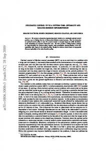
Fig. 1. The arc-flag method together with a separator partition. The labelled (gray) arc only leads to red and yellow nodes. A search with targets in green, black or white regions can ignore this arc.

The space requirement of the preprocessed data is O(pm) for p regions because we have to store one flag for each region and arc. There is a clear trade-off between speedup factor and space requirement. Depending on the chosen partition, one can regard the arc-flag acceleration of shortest path computation as an interpolation between no precomputed information at all (p = 1) and complete precomputation by determining all possible shortest paths of the graph (p = n). Thus, in theory, we can get as close as possible to the ideal shortest path search by increasing the number of regions in the partition (’ideal’ means that the shortest path algorithm visits only arcs that belong to the shortest path itself). Obviously, an increase in the number of regions also entails an increase in preprocessing time and space consumption. However, in practice, even for p  n we achieve an average search space that is at most 4 times the number of arcs in the shortest path. In fact, the number of regions can be kept of moderate size while one still achieves good speedups: about 225 regions on graphs with up to 1M nodes and 2.5M arcs deliver a speedup of up to 1,470. It is possible within the framework of the arc-flag speedup technique to use a single region for each of the most important nodes. Storing all shortest paths to important nodes can therefore be realized without any additional implementation effort. It is common practice in many applications to cache the shortest paths to the most important nodes in the graph.

3 3.1

The Preprocessing The Preprocessing with All-Pairs Shortest Path

We have to calculate the arc-flag vectors for all arcs. This can be done by computing two shortest path trees for every arc a ∈ A: a one-to-all shortest path computation from the head and from the tail node of arc a. The computation is done by a standard Dijkstra algorithm which stops when all nodes in the graph are permanently marked. For each node v ∈ V , we compute the difference between dh (v) and dt (v), the two distance labels in the shortest path trees of the head and the tail node of a. If the

7

difference |dh (v)−dt (v)| for node v is equal to the length `a of arc a, then we set the flag entry fa (rv ) to true. The running time of the preprocessing is dominated by the time it takes to compute 2m times a shortest path tree, which can be done in O(m + n log n) time each. For sparse graphs (m = O(n)), such as typical road networks, we get an overall worst-case time complexity of O(n2 log n). The preprocessing of the geometric containers (Schulz et al., 2000; Wagner and Willhalm, 2003) is done in a similar way by computing two shortest path trees per arc in the graph. Preprocessing our graphs (with 1M nodes and 2.5M arcs) by computing 2m times a shortest path tree would take weeks, but fortunately the arc-flags allow a much faster preprocessing, which is described in the following two sections 3.2 and 3.3. 3.2

The Preprocessing without All-Pairs Shortest Path

It is not necessary to compute all-pairs shortest paths to fill the flag vectors correctly. We can use the following insight: every shortest path from any node s to a region rt ∈ R has to enter the region rt at some arc. If s does not belong to rt , then there must be an arc (u, v) with ru 6= rt = rv ; a socalled boundary arc. We will see in Lemma 2, that in the preprocessing step it is sufficient to take into account only shortest paths to such nodes v which are tail nodes of boundary arcs. Such nodes will be called boundary nodes. Lemma 2 (Boundary nodes). Given a graph G = (V, A) and a partition of V in p regions by r : V → {1, . . . , p}. If the flag vectors fa for a ∈ A are computed with the set of shortest paths to boundary nodes only, then the flags vectors fa are a super set of the consistent target set Va0 . Proof. Let s and t be arbitrary but fixed nodes which are connected by a shortest path s = n1 , · · · , nk = t. Further, let s and t belong to different regions, i.e. rs 6= rt . By induction one can easily see that there exists an arc a = (ni , ni+1 ), 1 ≤ i < k, in this shortest path with rni 6= rni+1 = rt . The preprocessing which only considers shortest paths to boundary nodes would have considered the path from s to node ni+1 and hence it would have set the flag entry of region rt on all arcs of the shortest subpath s, · · · , ni+1 . The flag entry of region rt of the arcs between ni+1 and t are set by defintion, because the tail nodes of these arcs belong to the region rt . Since all flag entries corresponding to the target region rt are being set for all arcs on the shortest path s = n1 , · · · , nk = t, the modified Dijkstra algorithm finds this shortest path from s to t. We can now exploit this property: for a specified region r0 ∈ R and a boundary node b of r0 we calculate the set Tb of arcs a ∈ A with fa (r0 ) = true and where a is on a shortest path via b to any node in r0 . The reversed arcs corresponding to arcs in the set Tb form in fact a shortest path tree in the reverse graph Grev . A shortest path tree can be computed in time O(n log n) on sparse graphs. Therefore, we can compute the flag entries fa (r0 ) for region r0 for all nodes a ∈ A at once, if we compute a shortest path tree for each boundary node of r0 . This can be done in time O(kn log n) with k = |Br0 |, where Br0 is the boundary node set of r0 : Br0 = {v ∈ r0 | ∃(u, v) ∈ A such that ru 6= rv = r0 }. The number k of boundary nodes dependents on the partition of the nodes. When we search for an appropriate partition for the arc-flags, the following observation helps: the set of boundary arcs of all partitions r ∈ R represents a multi-way arc separator. Thus, if we want to minimize the number k of boundary nodes (and by this, minimize the preprocessing time), we need to find a minimum multi-way arc separator of the graph. We will see in Section 6, that a minimum multi-way arc separator partition is among the partitions on which the arc-flags achieve the best speedup results. However, as Section 4 shows, minimizing the number k of boundary arcs (i.e. separator arcs) is not the only objective when searching for a good partition for the arc-flags.

8

3.3

The Preprocessing with Pruned Shortest Path Trees

A straightforward implementation of the preprocessing phase of our method as it is presented in Section 3.1 leaves a lot of room for improvements. In the previous Section 3.2, we have presented an improved version, where for each single separator arc a backward Dijkstra search (i.e. a standard Dijkstra search in the reverse graph) has to be conducted to determine the flag vectors of all arcs in our graph. It is a simple observation that a contraction of all nodes of a region to a single super node and then performing one Dijkstra search from this super node does not supply correct arc-flags. Yet, when performing a backward Dijkstra search from two different separator arcs of a common region, the resulting shortest path trees show a strong similarity. More precisely, a large number of arcs that are contained in the first shortest path tree are as well contained in the second one. We call two separator arcs similar if they are in a geometrical sense ’closely together’ and point in a geometrically similar direction. We observed that for similar arcs the corresponding shortest path trees are almost identical, see Figure 11.

Fig. 2. We computed multi-way arc separator partitions of a subnetwork of the German road network (network data from the PTV Europe road network from the DIMACS Challenge homepage with 1M nodes and 2.5M arcs) with different numbers of regions (from 10 to 510). For each region r we analyzed the subgraph which is induced by those arcs a ∈ A which are on a shortest path to at least one node in r, i.e. fa (r) = true. For this induced graph, we identified subtrees and counted the number of arcs in all subtrees. These are the red entries in the diagram. Furthermore, we counted the number of all non-tree arcs in the induced graph. These are the blue entries. We did the counting for all regions of a partition. Now, the tree arcs (red) represent the preprocessing effort which we can save, because those arcs are on identical subtrees of all shortest path trees which we calculate per region. For those arcs, the shortest path tree calculation needs to be done only once per region.

Especially, in the more distant parts of the trees there are only a few differences between the two trees. One can take advantage of the similarity of the shortest path trees of similar arcs for speeding up the preprocessing version in Section 3.2. The Figures 2 and 10 show how much preprocessing effort we could save by exploiting the similarity between all the shortest path trees computed for one region.

9

In the following, we will describe the basic idea of how we can further improve the preprocessing from the last section. Take a separator arc a of the region under consideration. We denote by Ta the shortest path tree constructed by a backward Dijkstra search from the separator arc a. On the basis of the similarity observation made above, we can expect that the shortest path trees for all separator arcs of the same region that are similar to a will be almost identical to Ta . We identify now a small set of large subtrees Ta of Ta in an appropriate way and speedup the computation for any of the separator arcs s, similar to a, as follows. Let Tasub be a tree from the set Ta and r its root node. If Tasub is also a subtree of the shortest path tree of s, then, in the Dijkstra algorithm, we need to label only r permanently from s and can deduce from that the distance for each of the nodes of Tasub for free. So if each node v in Tasub knows its root node r then it can look up on demand its distance from s by adding up the distance label of r from s and its distance from r in Tasub . For the case that in Ts the shortest path to v is not via r in Tasub , we have to add some further structure: for each of the trees T in Ta we determine the set OT of outgoing arcs, i.e. the set of arcs that start in T and do not end in T . In the Dijkstra run for s, as soon as we label r, we insert all the arcs of OT into the heap together with the appropriate distance label inherited from r. Every time, the Dijkstra search from s reaches a node v via an arc from OTs the new label for v is compared with the previous v label (which v itself might have inherited from its root node r0 ). If this new label is better than the previous one, it is put in the Dijkstra heap and used for the further computation. However, if it is worse, it can be thrown away. In that way, the shortest path trees of all separator arcs similar to a can be computed much faster. Since this method is only applicable for arcs that are close together, the set Ta has to be recomputed for a separators arc a0 that is too far away from a and thus requires too many label propagations within the subtrees in Ta . Hence, this further improved preprocessing saves computational effort in different ways. On the one hand, labels that are dominated by inherited labels from root nodes can be deleted. On the other hand, the similarity between the search trees of similar separator arcs makes sure that most of the inner nodes of the subtrees from T are not directly labelled during the construction of the shortest path tree. Those inner nodes only inherit the label from the corresponding root node. Yet, various practical tests showed that although there is a big improvement in the number of Dijkstra-steps with this improved preprocessing method, the overhead for administering the additional data structure absorbs a large part of the corresponding saving in computation time. 3.4

The Preprocessing with Centralized Shortest Path Search

In the previously mentioned preprocessing approaches there had to be a single Dijkstra run for each of the boundary nodes of each region. As already pointed out in the last subsection large parts of the computed shortest path trees are almost identical. Hence, it seems to be very promising to “bundle together” the different Dijkstra runs for a given region. Yet, as mentioned before, it is not sufficient to just contract all boundary vertices to a single vertex and run a usual Dijkstra from there, since the anticipated graph is now not a tree anymore but rather a more complex graph. Our new approach is a so-called centralized shortest path algorithm. The basic idea is as follows: Instead of starting from just one of the boundary nodes we start the search from all boundary nodes of a region R at once. The boundary vertices are numbered b1 , ..., bk . Every vertex v of the graph is assigned a label, consisting of an array A of values. Entry A[i] stands for the length of the currently shortest path from boundary vertex bi to v. Furthermore, there is a heap containing those vertices that have been visited by the shortest path search and that wait to propagate their labels to their neighbors. Initially, for each of the boundary vertices bi the entry A[i] is set to 0 and for all j 6= i A[j] is set to the distance from bj to bi within the current region R. For all other vertices outside R all entries of A

10

are set to infinity. Each vertex v in the heap also carries a key k(v) which is used for sorting. Now the algorithm proceeds very much like a normal labeling algorithm by extracting the minimal element v from the heap (minimal with respect to the key value k) and propagating its label to the neighboring vertices. Let w be such a neighbor. We now update the whole label array of w by using the label array of v by adding the length of the corresponding arc (v, w) to each of the entries of the array A of v and comparing it to the values of the array of y; domination it defined as usual. A crucial role in the speed-up of this method in comparison to the previously mentioned preprocessing approaches is the choice of the key value k(v). One option is to take the minimum over all entries of A as key value for each vertex. With this choice the centralized shortest path algorithm behaves very much like k parallel Dijkstra algorithms. The label front moves very uniformly and does not prioritize any of the boundary vertices. A much better choice for the key is a kind of “quality based” value: We would like to prefer those labels that dominated many values in the previous step. To determine this, we account for each vertex w the number of entries of A in which there was an improvement (i.e. domination) since the last label propagation from w; this number is called domination value. The key value consists now of two parts, the domination value and the minimum over all entries of A, where the domination value shall be the dominant one. With this key setting there is no uniform label-front anymore. In fact, there will be a very interesting effect of this choice, that ensures that the search is quite similar to what we suggested in the previous subsection: In the first number of steps the algorithm determines all those edges of the graph that are on a shortest path to the first selected boundary vertex, since all other boundary vertices have domination value 0. When this search is completely finished the other boundary vertices come into play, one after another, each profitting from the quality of the previously computed labels. Our tests showed that the preprocessing phase can be accelerated very much (depending on the instance by about a factor of 100). However, the drawback of this method is the extremely high memory usage. Every single vertex of the network has to carry a label of size k, the number of boundary vertices of the current region. This issue can be dealt with in different ways. One option is to consider not all boundary vertices of the current region at once but rather partition it in smaller sets of boundary vertices and let the algorithm run for each of them. Another option is to keep the labels only for a subset of the vertices of the whole graph. This can be done by letting the algorithm propagate the labels only up to a certain distance from the current region and only let it run further when all the labels have reached this distance. Then all the labels having smaller distance can be ignored since there arc-flag is already determined and there will be no label going back to them during the run of the algorithm.

4

Which Partiton?

The arc-flag acceleration method uses a partition of the graph to precompute information on whether an arc is useful for a shortest path search. Any possible partition can be used for the technique and the accelerated Dijkstra algorithm will always return a correct shortest path, as Lemma 1 proves. However, different partitions do lead to different speedups of the Dijkstra algorithm. As an example, when we take a multi-way arc separator partition instead of a rectangular grid partition the preprocessing time can be reduced by a factor of 2, but at the same time we obtain up to 7 times larger acceleration factors with the separator partition. The question is, which partitions lead to the best query speedups. There are a number of objectives which a good partition should fullfil: first, the number of separator arcs should be small, because the preprocessing time directly depents on this number. Second, the size of partitions should be balanced. With almost equally sized regions the ’load’ per entry in a flag vector is balanced, i.e. each flag is ’responsible’ for the same amount of possible target nodes. Third, the number of almost full flag vectors should be minimal. For instance, for the partitions that

11

we presented almost one third of the flag vectors have more than 90% true entries, see Figure 15 (in the appendix). However, a full flag vector means that we almost never can exclude the corresponding arc during a accelerated Dijkstra search. Fourth, the partition should approximate in a geometric sense the consistent target set for each arc as closely as possible, see Figure 12 (in the appendix). Together with Birk Sch¨utz, Dorothea Wagner and Thomas Willhalm we studied different partitions in combination with the arc-flag approach extensively, see (M¨ohring et al., 2006). Therefore, in this section, we will only present a summary of these results. Most of these algorithms need a 2D layout of the graph, except for the multi-way arc separator algorithm used by METIS. The partition algorithms based on a 2D layout can easily be adapted to higher dimensions. For the arc-flag approach itself no layout of the graph is necessary as long as one can provide a partition for a given graph. Rectangular partition (grid). Probably the easiest way to partition a graph with a 2D layout is to define the regions with a x × y grid of the bounding-box. More precisely, we denote with (`, t) the top-left coordinate of the bounding-box of the 2D layout of the graph and with (r, b) the bottomright one. Furthermore, we define w = r − ` as the width and h = t − b as the height of the layout. The grid cell or region  Gi,j with 0 ≤ i < x, 0 ≤  j < y is now defined as the rectangle  ` + i · wx ; ` + (i + 1) · wx × b + j · hy ; b + (j + 1) · hy . Nodes on a grid line are assigned to one of the neighboring grid cells. Figure 13(a) (in the appendix) shows an example of a 7 × 5 grid. The rectangular or grid partition method uses only the bounding-box of the graph. All other properties like the structure of the graph or the density of nodes are ignored and hence it is not surprising that this method is not among the best partitions for our application. In fact, the grid partition always has the worst results in our experiments. Since earlier work on the arc-flag method (Lauther, 2004) used the grid partition, we take it as a baseline and compare all other partition algorithms with it. Quad-trees. A quad-tree is a data structure for storing points in the plane. Quad-trees are typically used in algorithmic geometry for range queries since they support fast access to nearest neighbor points. Further applications are in computer graphics, image analysis, and geographic information systems. Quad-trees can be generalized to higher dimensions – for 3D they are called oct-trees. Let P be a set of n points in the plane, r0 its quadratic bounding-box, then the data structure quad-tree is recursively defined as follows (see Figure 14 in the appendix): – Root v0 corresponds to the bounding region r0 . – Region r0 and all other regions ri are recursively divided into four quadrants, while they contain more than one point of P . The four quadratic subregions of ri are subnodes of vi in the quad-tree. The leaves of a quad-tree form a subdivision of the bounding-box r0 . Even more, the leaves of every subtree contain the root from such a subdivision. Since, for our application, we do not want to create a separate region for each node, we use a subtree of the quad-tree. More precisely, we define an upper bound b ∈ N of points in a region and stop the division if a region contains fewer points than the bound b. The result is a partition of our graph where each region contains at most b nodes. Figure 13(b) shows such a partition with 32 regions. In contrast to the grid partition, this partition reflects the geometry of the graph better: dense parts will be divided into more regions than sparse parts. The regions generated by this partition have almost balanced size, but the arc separator set can be large. kd-Trees In the construction of a quad-tree, a region is divided into four equally sized subregions. However, equally sized subregions do not take the distribution of the points into account. This quadtree division can therefore be extended to more general subdivision schemes, the so-called kd-trees.

12

In the construction of a kd-tree, the plane is recursively divided in a similar way as for a quad-tree. In contrast to a quad-tree, the underlying rectangle is decomposed into two halves by a straight line parallel to an axis. The axes alternate in the order x, y, x, y, . . .. The positions of the dividing line can depend on the data. Frequently used positions are given by the center of the rectangle (standard kd-tree), the average, or the median of the points inside. If the median of points in general position is used, the partition has always 2q regions, q ∈ N, and the region sizes are balanced. Figure 13(c) (in the appendix) shows a result for the median and 32 regions. In applications with higher dimensions, the partition axes are not cycled but the dimension with the largest variance is used. Experiments on road networks showed that the kd-tree with median partition position usually leads to the best results, Figure 13(c) (in the appendix). Therefore, we only used this method as a representative for this partition class. If the median of the points is used, at every decomposition one node of the graph lies exactly on the boundary of two regions. For these nodes it is worthwhile to check whether all neighbors of that node have their positions in the other region. If yes, the node can be transferred to the other region and will not become a boundary node. The median of the nodes can be computed in linear time with the median of medians algorithm (Cormen et al., 2001). Since the running time of the preprocessing is dominated by the shortest path tree computations after the partition of the graph, we decided to use standard algorithms: sorting the nodes and taking the mean. As an example, the kd-tree partition with 64 regions for our test graph with 1M nodes and 2.5M arcs was calculated in 175 sec. Multi-way arc separator. A partition of the graph into k almost equally sized regions with a small (almost minimal) arc separator set can be computed by the multi-way arc separator algorithms presented in (Karypis and Kumar, 1998). An efficient implementation of the algorithms can be obtained free of charge from (Karypis, 1995). The algorithms implemented in METIS are based on multilevel recursive-bisection, multilevel k-way, and multi-constraint partition schemes. The METIS partition method has several advantages for our application: it does not need a layout of the graph and is therefore the most general partition method among those presented in the present article. The number of arcs in the separator is noticeably smaller than in the other partition methods. The size of the regions is balanced and the number of full flag vectors is among the smallest of all the partitions we studied. Figure 13(d) (in the appendix) shows a partition of a graph generated by METIS.

5

Space Consumption—Coarse vs Fine Partition

An analysis of the calculated flag vectors shows that (depending on the partition) on average more than 50% of the flag vectors have only 10% true entries, see Figure 15 and Table 2 (both in the appendix). The high amount of almost empty flag vectors justifies the idea for a compression of the vectors. It is important that the decompression algorithm is very fast – otherwise the speedup of the running time will be lost. The two- and more level technique, we describe in this section, is a suitable lossy compression method for the flag vector entries. Let us have a closer look at the search space generated by the arc-flag accelerated Dijkstra search to get an idea of how to compress the arc-flags: as illustrated in Figure 16(a) (in the appendix), the accelerated Dijkstra search reduces the search space at the beginning of the search, but once the target region has been reached, almost all nodes and arcs are visited. This is not very surprising, if we consider that usually all arcs of a region were assigned the region-flag of their own region. We could deal with this problem by using a finer partition of the graph but this would lead to larger flag vectors at each arc (requiring more memory and a longer preprocessing). Take the following example: if we use a fine 15 × 15 grid instead of a coarse 5 × 5 grid (i.e. each coarse region would be split into 9

13

additional finer regions), then the preprocessed data will increase from 25 flags (in the coarse case) to 225 flags (in the fine case) per arc. Note that the additional information of the fine grid is mainly needed for arcs close to the target node, e.g. arcs in the target region of the coarse grid. This leads to the idea of splitting each region of the coarse partition into a set of smaller regions (see Figure 16(b) in the appendix). For each such set of smaller regions (i.e. for each fine partition of a region from the coarse partition) we compute and store additional flag vectors only for those arcs inside the same coarse region. More precisely, we partition the graph induced by the nodes in the (coarse) regions and perform (for each induced graph) another preprocessing where we calculated another flag vector for each arc in the induced graphs. The entries of this additional flag vector per arc are associated with the fine regions of the same coarse region. Hence, each arc gets two flag vectors assigned: one for the coarse partition and one for the fine partition of the coarse region to which the arc belongs. This approach can be iterated to more than 2 levels of finer partitionings. The advantage of this two-level partition approach is that the preprocessed data is much smaller than for a fine one-level partition. This is because the second flag vector of an arc a is relevant (i.e. computed, stored, and evaluated) only for the coarse region to which the arc a belongs. In the example above, the two-level approach would need only 34 flags per arc (instead of 225). The difference between the search spaces of the arc-flag accelerated Dijkstra search with the one- and with the two-level partition is small. This is the case, because for the one-level partition the entries in flag vectors corresponding to faraway neighboring regions are similar to each other. Therefore, we are not loosing too much information from the one-level flag entries with the two-level partitions. The twolevel approach can be viewed as a (lossy) compression of the one-level flag vectors: we accumulate the flag entries for faraway regions. For the two-level partition approach only a slight modification of the search algorithm is required: until the target region is reached, everything remains unaffected, unnecessary arcs are ignored by using the flag vectors of level one. When the algorithm has entered the target region, the second-level flag vector provides further information on whether an arc can be ignored for the search of a shortest path to the target node. Preprocessing the arc-flags for the two-level approach takes slightly longer than for the one-level approach. However, almost the same speedups can be achieved with two-level partitions with only a fraction of the space consumption of the one-level partitions.

6

Experimental Setup and Computational Results

Implementation. We implemented the arc-flags in C++ using the GNU g++ compiler version 4.1 with the optimizing option ”-O4” on Linux 2.4/2.6 systems (SuSE 9.1). We did all computations on 64 bit AMD Opteron X2 Dual Core machines 2.2 GHz with 4 GB memory and 1 MB cache memory. Table 1 shows that our implementation of Dikstra’s Algorithm is by a factor 3.9 to 6.5 slower than the DIMACS implementation. One reason for that is that our implementation is thoroughly based on the Boost Graph Library (BGL). Apperently this slowed down our code a lot. In K¨ohler et al. (2005) we used our own graph datastructure instead of the BGL. Our Dijkstra implementation from K¨ohler et al. (2005) performs as well as the DIMACS implementation, but we will use the BGL-based code for the current paper since we didn’t had the time to switch back to our old code from K¨ohler et al. (2005). Instances. Currently we are heavily working on extensive experiments with the data from the DIMACS Challenge homepage, especially the road networks of Europe and USA. The present paper gives preliminary results on these networks and a subnetwork of the German road network that is part of the PTV Europe network from the DIMACS Challenge homepage. Most of these results on

14 name

| nodes |

| edges |

dimacs [ms]

own [ms]

own/dimacs

NY 264346 733846 57.632 231.66 4.0 BAY 321270 800172 68.096 266.36 3.9 COL 435666 1057066 93.242 400.51 4.3 FLA 1070376 2712798 257.756 1390.51 5.4 NW 1207944 2840206 336.965 1592.72 4.7 NE 1524452 3897634 390.800 1878.12 4.8 CAL 1890814 4657740 488.319 2473.01 5.1 LKS 2758118 6885656 750.431 3331.92 4.4 E 3598622 8778112 1095.032 7163.35 6.5 W 6262103 15248144 2040.588 10173.3 5.0 Table 1. DIMACS benchmark software versus our plain Dijkstra implementaion using the Boost Graph Library (BGL).

the German road network already appeared in (M¨ohring et al., 2006, 2005). Therefore, we focus on a summary to prove the preformance of the arc-flag method, see Figures 3 and 4. For the German road subnetworks we have mainly used the networks in Table 3 (in the appendix). Each arc in these networks has a nonnegative integer geographic length. For each network instance we randomly generated up to 2,500 route requests. The measured speed-up factors and running times are averaged over all computed requests. We did the shortest path computations in Figure 3 with the following acceleration methods and compared them to Dijkstra’s standard algorithm: a hierarchical approach together with a separator heuristic, see M¨ohring et al. (2005) for details, the arc-flag approach together with a rectangular partition and a multi-way arc separator partition. The arc separators were computed with METIS (Karypis, 1995). Combining the bi-directed search and the arc-flag method with an arc separator partition by METIS was the most successful method in our tests with a speed-up of up to 1,470. Figure 4 compares the results of the different partitioning methods on four road networks (see Table 3 in the appendix on details of the networks). The size of the preprocessed data is nearly the same for all algorithms (80 bits). The same size could not be realized since, for instance, kd-tree partitions always have size 2q , q ∈ N. Table 5 (in the appendix) shows the partitions we used for the comparison. Our preliminary results on the road networks of Europe and USA are given in the following figures.

7

Discussion and Outlook

We presented a number of improvements of the basic variant of the arc-flag acceleration (Lauther, 1997, 2004) for speeding up the P2P shortest path search on static networks. Arc flags are a modification to the standard Dijkstra algorithm and are used to avoid exploring unnecessary paths during shortest path computation. We showed that the improved arc-flags achieve speedups of P2P shortest path queries of more than 1,470 on a subnetwork of the German road network with 1M node and 2.5M arcs using 450 bits of additional information per arc. The orginal arc-flag version of Lauther (2004) is only capable of obtaining speedups of up to 64 on the European truck driver’s road network with 0.3M nodes, 0.5M arcs and 278 bits of additional information per arc. Even the latest version of the highway hierarchies by Sanders and Schultes (2006) does not compete with the speedups of the improved version of the arc-flags (Schultes, 2006): a speedup of 1,121 is obtained by the highway hierarchies on the same German road network with 1M node and 2.5M arcs using 450 bits of additional information per arc.

15

hierarchical approach with sep. heuristic arc-flags with rect. part. (225 regions) arc-flags with sep. part. (225 regions) arc-flags with sep. part. & bidi (225 regions)

1400 1200

speedup factor

1000 800 600 400 200 0 AA

BY

HS

NO NW OS network instances

TH

GH

GR

Fig. 3. Speedups on all networks compared to the plain Dijkstra algorithms (speedup 1). Results are shown for a hierarchical approach together with a separator heuristic, the arc-flags with a rectangular partition (225 regions), the arc-flags with a separator partition (225 regions), and the arc-flags with a separator partition combined with a bi-directed search (225 regions for each direction).

search space [nodes touched]

16000

road network AA road network OS road network BW road network BY

14000 12000 10000 8000 6000 4000 2000

Bi2LevelKD(80)

BiMETIS(80)

BiKD(64)

BiGrid(85)

2LevelMETIS(80)

2LevelKd(80)

2LevelGrid(80)

METIS(80)

KdTree(64)

Grid(81)

0

Fig. 4. Average search spaces for most of the algorithms we implemented on four road networks (see Tables 4 and 5 in the appendix for details). The numbers of bits of additional information per arc are given in brackets.

16

0.26 0.22

0.24

time in sec

0.28

0.30

USA−road−t.E with 300 partitions

rank11

rank12

rank13

rank14

rank15

rank16

rank17

rank18

rank19

rank20

rank21

dijkstra rank

Fig. 5. Query times of a uni-directed Dijkstra search on network E for 1000 demands and 300 partitions.

0.12 0.08

0.10

time in sec

0.14

0.16

0.18

USA−road−t.NW with 100 partitions

rank10

rank11

rank12

rank13

rank14

rank15

rank16

rank17

rank18

rank19

rank20

dijkstra rank

Fig. 6. Query times of a uni-directed Dijkstra search on network NW for 1000 demands and 100 partitions.

17

0.10 0.08

time in sec

0.12

0.14

USA−road−t.NW with 250 partitions

rank10

rank11

rank12

rank13

rank14

rank15

rank16

rank17

rank18

rank19

rank20

dijkstra rank

Fig. 7. Query times of a uni-directed Dijkstra search on network NW for 1000 demands and 250 partitions.

0.10 0.07

0.08

0.09

time in sec

0.11

0.12

0.13

USA−road−t.NW with 490 partitions

rank10

rank11

rank12

rank13

rank14

rank15

rank16

rank17

rank18

rank19

rank20

dijkstra rank

Fig. 8. Query times of a uni-directed Dijkstra search on network NW for 1000 demands and 490 partitions.

18

0.50 0.40

0.45

time in sec

0.55

0.60

0.65

USA−road−t.W with 100 partitions

rank10 rank11 rank12 rank13 rank14 rank15 rank16 rank17 rank18 rank19 rank20 rank21 rank22 dijkstra rank

Fig. 9. Query times of a uni-directed Dijkstra search on network W for 1000 demands and 100 partitions.

The point that leaves room for improvements with the arc-flags is the preprocessing: for instance, precomputing the highway hierarchies on the our German road network example with 1M node and 2.5M arcs can be done within 1 minute, while preprocessing the arc-flags takes up to 120 minutes on this network. Section 3.3 hinted at a new idea for a fast preprocessing of the flag vectors. In this preprocessing, we have to compute at least one full shortest path tree per region. This would give us a straightforward lower bound on the running time, because computing a full shortest path tree on a subnetwork of the German road network takes at most 1 second. From our work on the German road network example we know that we need a partitioning with 225 regions for forward and backward search on that network. On this basis, we can assume a lower time bound on the preprocessing of 7.5 minutes for German road network example. The new preprocessing idea from Section 3.3 would bring us very close to this lower bound of 7.5 minutes and therefore already very close the 1 minute of preprocessing necessary for the highway hierarchies (Schultes, 2006) on the same network. Using our multi-level idea (Section 5) we would then be able to reduce the space consumption of 450 bits per arc to only 68 bits. At the same time, we would gain almost the same acceleration factor of 1,470, and even more importantly: the preprocessing effort would be reduced much further. The reason for this is that with the two-level partitioning we are works on coarser partitionings (with much less numbers of regions) and smaller (induced) graphs (for the second level arc-flags). On this basis, future research could improve the arc-flags method even further.

Bibliography

Cormen, Thomas H., Charles E. Leiserson, Ronald L. Rivest, and Cliff Stein (2001, September). Introduction to Algorithms (2nd ed.). Cambridge, MA, USA: The MIT Press. Dijkstra, Edsger Wybe (1959). A note on two problems in connexion with graphs. In Numerische Mathematik, Volume 1, pp. 269–271. Amsterdam, The Netherlands: Mathematisch Centrum. DIMACS (2006). 9th Implementation Challenge — Shortest Paths. http://www.dis. uniroma1.it/˜challenge9. Enders, Reinhard and Ulrich Lauther (1999, May). Method and device for computer assisted graph processing. http://gauss.ffii.org/PatentView/EP1027578. Siemens AG. Fredman, Michael L. and Robert Endre Tarjan (1987). Fibonacci heaps and their uses in improved network optimization algorithms. Journal of the Association for Computing Machinery 34(3), 596– 615. Goldberg, Andrew V. and Chris Harrelson (2005). Computing the shortest path: A∗ search meets graph theory. In Adam Buchsbaum (Ed.), Proceedings of the 16th Annual ACM-SIAM Symposium on Discrete Algorithms (SODA), Vancouver, BC, Philadelphia, PA, USA, pp. 156–165. SIAM. Goldberg, Andrew V., Haim Kaplan, and Renato Fonseca Werneck (2006). Reach for A∗ : Efficient point-to-point shortest path algorithms. In Proceedings of the 8th Workshop on Algorithm Engineering and Experiments (ALENEX). SIAM. To appear. Goldberg, Andrew V. and Renato Fonseca Werneck (2005). Computing point-to-point shortest paths from external memory. In Proceedings of the 7th Workshop on Algorithm Engineering and Experiments (ALENEX), pp. 26–40. SIAM. Gutman, Ronald J. (2004). Reach-based routing: A new approach to shortest path algorithms optimized for road networks. In Lars Arge, Giuseppe F. Italiano, and Robert Sedgewick (Eds.), Proceedings of the 6th Workshop on Algorithm Engineering and Experiments (ALENEX) and the First Workshop on Analytic Algorithmics and Combinatorics (ANALCO), New Orleans, LA, USA, Philadelphia, PA, USA, pp. 100–111. SIAM. Johnson, Donald B. (1977). Efficient algorithms for shortest paths in sparse networks. Journal of the Association for Computing Machinery 24(1), 1–13. Karypis, George (1995). METIS: Family of multilevel partitioning algorithms. http:// www-users.cs.umn.edu/˜karypis/metis/. Karypis, George and Vipin Kumar (1998, August). A fast and high quality multilevel scheme for partitioning irregular graphs. SIAM Journal on Scientific Computing 20(1), 359–392. Knopp, Sebastian, Peter Sanders, Dominik Schultes, Frank Schulz, and Dorothea Wagner (2006). Fast computation of distance tables using highway hierarchies. Technical report, Faculty of Informatics, University of Karlsruhe. K¨ohler, Ekkehard, Rolf H. M¨ohring, and Heiko Schilling (2005). Acceleration of shortest path and constrained shortest path computation. In Sotiris E. Nikoletseas (Ed.), In Proceedings of the 4th International Workshop on Experimental and Efficient Algorithms (WEA), Volume 3503 of Lecture Notes in Computer Science, Heidelberg, Germany, pp. 126–138. Springer. Lauther, Ulrich (1997). Slow preprocessing of graphs for extremely fast shortest path calculations. Lecture at the Workshop on Computational Integer Programming at ZIB. Lauther, Ulrich (2004). An extremely fast, exact algorithm for finding shortest paths in static networks with geographical background. In Martin Raubal, Adam Sliwinski, and Werner Kuhn (Eds.), Geoinformation und Mobilit¨at - von der Forschung zur praktischen Anwendung, Volume 22 of IfGI prints, M¨unster, Germany, pp. 219–230. Institut f¨ur Geoinformatik, Westf¨alische Wilhelms-Universit¨at.

20

Maue, Jens, Peter Sanders, and Domagoj Matijevic (2006). Goal directed shortest path queries using ` precomputed cluster distances. In Carme Alvarez and Maria J. Serna (Eds.), Proceedings of the 5th International Workshop on Experimental Algorithms (WEA), Volume 4007 of Lecture Notes in Computer Science, pp. 316–327. Springer. M¨ohring, Rolf H., Heiko Schilling, Birk Sch¨utz, Dorothea Wagner, and Thomas Willhalm (2005). Partitioning graphs to speed up dijkstra’s algorithm. In Sotiris E. Nikoletseas (Ed.), Proceedings of the 4th International Workshop on Experimental and Efficient Algorithms (WEA), Volume 3503 of Lecture Notes in Computer Science, Heidelberg, Germany, pp. 189–202. Springer. M¨ohring, Rolf H., Heiko Schilling, Birk Sch¨utz, Dorothea Wagner, and Thomas Willhalm (2006). Partitioning graphs to speed up dijkstra’s algorithm. ACM Journal of Experimental Algorithms (JEA) 12, 1–29. To appear. Sanders, Peter and Dominik Schultes (2005). Highway hierarchies hasten exact shortest path queries. In Gerth Stølting Brodal and Stefano Leonardi (Eds.), Proceedings of the 13th Annual European Symposium (ESA), Volume 3669 of Lecture Notes in Computer Science, pp. 568–579. Springer. Sanders, Peter and Dominik Schultes (2006, September). Highway hierarchies hasten exact shortest path queries. In Proceedings of the 14th Annual European Symposium (ESA). To Appear. Schultes, Dominik (2006, August). Personal communication. Schulz, Frank, Dorothea Wagner, and Karsten Weihe (2000). Dijkstra’s algorithm on-line: An empirical case study from public railroad transport. ACM Journal of Experimental Algorithms 5, 12. Wagner, Dorothea and Thomas Willhalm (2003). Geometric speed-up techniques for finding shortest paths in large sparse graphs. In Giuseppe Di Battista and Uri Zwick (Eds.), Algorithms - ESA 2003, 11th Annual European Symposium, Budapest, Hungary, Heidelberg, Germany, pp. 776–787. Springer-Verlag, Lecture Notes in Computer Science, vol. 2832. Willhalm, Thomas (2005). Engineering Shortest Paths and Layout Algorithms for Large Graphs. Ph. D. thesis, Faculty of Informatics, University of Karlsruhe.

21

A

The Preprocessing

Fig. 10. We computed a multi-way arc separator partition of the Luxembourg road network (network data from the PTV Europe road network from the DIMACS Challenge homepage). The green arcs belong to the same region r. We analyzed for region r the subgraph which is induced by those arcs a ∈ A which are on a shortest path to at least one node from r, i.e. fa (r) = true. For this induced graph, we identified subtrees. These are the red arcs in the figure. The blue arcs are the non-tree arcs in the induced graph. The gray arcs do not belong to the induced subgraph, i.e. f (r) = true. Now, the tree arcs (red) represent the preprocessing effort which we can save, because those arcs are on identical subtrees of all shortest path trees that we calculate for region r. For those arcs, the shortest path tree calculation needs to be done only once for region r.

22

Fig. 11. We computed a multi-way arc separator partition of the Luxembourg road network (network data from the PTV Europe road network from the DIMACS Challenge homepage). The green arcs belong to the same region r. We calculated the shortest path trees for two similar separator arcs a1 and a2 of region r. The blue and yellow arcs in the figure represent the two shortest path trees and the red arcs are the identical shortest path subtrees of a1 and a2 . The gray arcs do not belong to any of the trees.

B

Which Partiton?

23

a fa 1 1 1 1 1 1 1 0 0 0 0 0 0 0 0 0

Fig. 12. The arc-flag method together with a rectangular partition. At each arc a, a flag vector fa is stored such that fa (i) indicates if a is on a shortest path into region i. The set of regions for which fa (i) = true (yellow regions in the figure) approximates in a geometrical sense the consistent target set of arc a, i.e. the set of nodes to which a shortest path starting with a exists.

(a) Rectangular partition (35 regions)

(b) Quad-tree (34 regions)

(c) kd-Tree (32 regions)

(d) METIS (32 regions).

Fig. 13. Germany with four different partitions.

Fig. 14. Example of a Quad-Tree. Each region is recursively divided until each region contains only one point.

24

C

Space Consumtion—Coarse vs Fine Partition

Table 2. Analysis of the arc-flags: kdTree(n) and METIS(n) are partition algorithms of size n. For 80% of the arcs, either almost none (< 10 %) or nearly all (> 95 %) flags of the corresponding flag vector have been set to true. network number of arcs AA AA AA BY BY

920,000 920,000 920,000 2,534,000 2,534,000

algorithm KdTree(32) KdTree(64) METIS(80) KdTree(32) KdTree(64)

600000

< 10 % > 95 %

351,255 443,600 312,021 334,533 470,818 294,664 346,935 468,101 290,332 960,779 1,171,877 854,670 913,605 1,209,353 799,206

arc-flags with rectangle partition arc-flags with separator partition

500000 number of arcs

=1

400000 300000 200000 100000 0 0 − 10

20 − 30

40 − 50

60 − 70

80 − 90

fill rate of arc-flag vectors [%] Fig. 15. Statistics of the fill rate of the flag vectors on instance OS (1,169,000 arcs). The y-axis shows the number of arcs for which the corresponding flag vector has a certain fill rate, while the x-axis shows the percentages of different fill rates. For instance, an arc a has a flag vector with fill rate 30% if 3 out of 10 flags in the vector have been set to true.

25

(a) Without two-level arc-flags a search visits almost all arcs in the target region (lower left gray point).

(b) For each arc a, a flag vector is stored for the coarse 5 × 5 grid and a flag vector for a fine 3 × 3 grid in the same coarse region as the arc a.

Fig. 16. Two-level partition.

D

Experimental Setup and Computational Results

26

Table 3. Characteristics of the road networks used in the experiments. Most of them are part of the PTV Europe network from the DIMACS Challenge homepage. name description

# nodes

# arcs

German Railway 14,938 German Highway 53,315 North Rhine362,554 Westphalia south TH Thuringia 422,917 OS Berlin, 474,431 Brandenburg, Saxony, Saxony-Anhalt, Mecklenburg NW North RhineWestphalia north 560,865 NO Lower Saxony, 655,192 Schleswig-Holstein, Hamburg, Bremen HS Hesse, Saarland, Rhineland-Palatinate 675,465 BY Bavaria 1,045,567

32,520 109,540 920,464

GR GH AA

1,030,148 1,169,224

1,410,076 1,611,148

1,696,054 2,533,612

Table 4. Overview of the tested algorithms. Name

Description

Parameter

Grid KdTree METIS 2LevelGrid 2LevelKdTree

c × c grid over graph layout kd-tree concerning coordinates of nodes partition generated by METIS c × c grid coarse grid, g × g fine grid coarse kd-tree and fine kd-tree

2LevelMETIS

coarse METIS and fine METIS

BiGrid

bi-directed grid

BiKdTree Bi2LevelGrid Bi2LevelKdTree BiMETIS

bi-directed kd-tree bi-directed 2LevelGrid bi-directed 2LevelKdTree bi-directed METIS

c depth of kd-tree number of regions c and g depth of coarse and fine kd-tree number of coarse and fine regions size of forward and backward grid depth of kd-trees sizes of grids depth of kd-trees number of forward and backward regions

27

Table 5. Partitions with nearly the same preprocessed data size of 80 bit. Name of partitioning Grid KdTree METIS 2LevelGrid 2LevelKd 2LevelMETIS BiGrid BiKd BiMETIS Bi2LevelGrid Bi2LevelKd

forward backward bits per arc 1st level 2nd level 1st level 2nd level 9×9 64 80 8×8 64 72 7×7 32 40 6×6 32

4×4 16 8 2×2 8

6×6 32 40 6×6 32

2×2 8

81 64 80 80 80 80 85 64 80 80 80