Shortest Path versus Multi-Hub Routing in Networks with ... - arXiv

Shortest Path versus Multi-Hub Routing in Networks with Uncertain Demand Alexandre Fr´echette∗ , F. Bruce Shepherd† , Marina K. Thottan‡ and Peter J. Winzer§ ∗ Department

of Computer Science, University of British Columbia, Canada1 of Mathematics and Statistics, McGill University, Canada ‡ Bell Labs, Emerging Technology Division, Murray Hill, NJ, USA § Bell Labs, Optical Transmission and Networks Research Department, Holmdel, NJ, USA

arXiv:1302.7028v1 [cs.NI] 27 Feb 2013

† Department

Abstract—We study a class of robust network design problems motivated by the need to scale core networks to meet increasingly dynamic capacity demands. Past work has focused on designing the network to support all hose matrices (all matrices not exceeding marginal bounds at the nodes). This model may be too conservative if additional information on traffic patterns is available. Another extreme is the fixed demand model, where one designs the network to support peak point-to-point demands. We introduce a capped hose model to explore a broader range of traffic matrices which includes the above two as special cases. It is known that optimal designs for the hose model are always determined by single-hub routing, and for the fixeddemand model are based on shortest-path routing. We shed light on the wider space of capped hose matrices in order to see which traffic models are more shortest path-like as opposed to hub-like. To address the space in between, we use hierarchical multi-hub routing templates, a generalization of hub and tree routing. In particular, we show that by adding peak capacities into the hose model, the single-hub tree-routing template is no longer cost-effective. This initiates the study of a class of robust network design (RND) problems restricted to these templates. Our empirical analysis is based on a heuristic for this new hierarchical RND problem. We also propose that it is possible to define a routing indicator that accounts for the strengths of the marginals and peak demands and use this information to choose the appropriate routing template. We benchmark our approach against other well-known routing templates, using representative carrier networks and a variety of different capped hose traffic demands, parameterized by the relative importance of their marginals as opposed to their point-to-point peak demands. This study also reveals conditions under which multi-hub routing gives improvements over single-hub and shortest-path routings.

I. I NTRODUCTION Traditional communication networks are designed based on knowledge of an expected traffic demand matrix that specifies the aggregate traffic between every pair of nodes in the network and evolves slowly, over a time scale of months or years. In an era of data-dominant communication networks with dynamic demand patterns, this traditionnal network design methodology loses its cost-effectiveness. For instance, in emerging data services such as YouTube, user generated video content and flash crowds are triggering an increasing amount of dynamic uncertainty in the traffic demand. One specific concern is that the real-time estimation of the dynamically changing traffic patterns in large data networks is intractable. 1 This author’s work was done while studying at McGill University, and with generous funding from NSERC Discovery Grant No. 212567.

Moreover, a pessimistic approach of designing for peak pointto-point demands (also referred to as the fixed-demand model) throws away critical information for achieving “cost-sharing” between the varying demand patterns that arise over time. A traffic model that has gained considerable popularity in coping with dynamic demands is the hose model [1], [2]. In this model, only bounds on the ingress/egress traffic of the nodes are known. These bounds (called marginals) are physically represented by the various interface speeds of networking hardware at any given node. The actually encountered pointto-point traffic distributions are subject to dynamic variations during network operation, but the network is provisioned to be able to support any possible pattern meeting the ingress/egress bounds. Formally, in the symmetric (undirected) demand case, the space of hose matrices PHU consists of symmetric matrices D satisfying the bound: j Dij ≤ U (i) for each node i, with marginal U (i); in addition, the main diagonal of these matrices is typically set to zero, reflecting the fact that nodes generally do not send traffic to themselves. However, the flexibility of the hose model can also be a drawback since totally random demand matrices rarely ever occur in practice, and the operator usually has additional at least some a priori information about the traffic pattern. For instance, it may happen that there exists some additional peak demand U (i, j) between nodes i, j, i.e. Dij ≤ U (i, j). We call this union of marginals and peak demands the capped hose model. Depending on the choice of U (i, j), the space of traffic patterns spanned by the capped hose model ranges from purely deterministic point-to-point demands (Dij = U (i, j)) to the space of unconstrained hose traffic (U (i, j) = min(U (i), U (j))). Designing a network for the capped hose model hence avoids the massive overprovisioning that may arise for unconstrained hose traffic [3]. In order to solve the routing problem for the capped hose model, we propose the use of a class of oblivious routing strategies, called hierarchical hubbing routing templates (HH), which generalizes the popular hub and tree routing templates. We give empirical results based on a heuristic for the corresponding new class of robust network design (RND) problems. In order to quantify the extent of the space of traffic matrices spanned by the capped hose model, we propose indicators (marginal versus peak strength measures) that could be used as a predictor for which traffic scenarios favour a shortest path routing (SP), and which favour HH routings. We also show

2

that HH is often superior in general to both SP and hub routing (HUB), in terms of network design (considering both link and node costs). A. Summary of Main Contributions 1) We systematically study the capped hose model as a generalization of the fixed-demand and the unconstrained hose models. This allows tapping into a whole range of practically relevant traffic scenarios. 2) We initiate a formal study of a class of RND problems based on oblivious HH routing templates, a generalization of tree and single-hub routing used by optimal virtual private networks (VPNs). We provide theoretical examples showing that SP is much cheaper than HH, and vice-versa. 3) We perform an empirical study (based on both randomly generated and real traffic data) on the space of new capped hose traffic polytopes. 4) Our initial empirical findings show that for most instances, HH is better than single-hub VPN, suggesting that multi-hubbing at different layers can be important for network cost savings. Empirical results suggest that for many instances HH is significantly better than SP. 5) We provide some initial understanding of which traffic scenarios favour SP-like, and which are more HH-like. This is achieved by introducing two metrics that quantify the strengths of the marginals and peak demands in the specification of a collection of traffic matrices. These indicators could be used as a predictor for which of the two routing templates, SP and HH, is better. II. T RAFFIC E NGINEERING FOR C ORE N ETWORKS A. Oblivious Routing and Routing Templates Apart from the traffic modelling complexities mentioned above, which form the basis for network infrastructure planning and design, there is a second operational complication arising in any network with dynamically changing traffic patterns: how should traffic be routed on an installed infrastructure? Since centralized or distributed control planes may not have the speed and flexibility to adapt dynamically to rapidly varying traffic patterns without the risk of inducing detrimental oscillations [4], the vast majority of today’s networks are designed based on the principle of oblivious routing, usually based on SP, both on the circuit and on the packet layer. Informally, Valiant [5] defined oblivious routing as “the route taken by each packet be determined entirely by itself. The other packets can only influence the rate at which the route is traversed.” Formally, this amounts to specifying a template: for each possible communicating pair of nodes i, j, one specifies a path Pij .2 Traffic from node i to j is always routed on Pij independent of any other demands or congestion in the network. Oblivious routing is attractive because it enables strictly local routing decisions. In contrast, stable nonoblivious routing would require a global network control plane 2 Valiant actually considered the randomized version and so the flows could be fractional.

performing path optimization on a time scale much faster than the congestion and traffic variation dynamics, which is impractical in most scenarios. For the fixed-demand traffic model, a minimum cost design is achieved using an oblivious SP routing template. Using SP for hose traffic, however, may result in significant over-provisioning of network resources (if blocking is to be avoided)[3]. On the other hand, it was proved in [6] that the optimal design (in the undirected setting) for the hose model is always induced by a tree routing template (i.e. there exists a network-specific tree, and the template is to use the path Pij in that tree between node i, j). In [2], [7] a simple polynomial-time algorithm was given to produce the optimal tree template. Their analysis shows that the resulting network (called a virtual private network - VPN) actually has enough capacity to support hub routing (HUB) within the tree. That is, there is a hub node h and enough capacity in the tree for each node to reserve a private circuit of size U (i) to h. We use HUB to denote such routing templates. B. The Capped Hose Model We now consider the class of capped hose matrices and the minimum cost network to support it. •

•

•

If P the node bounds U (i) are sufficiently large (at least j U (i, j)), then they impose no constraints on the routed demand. Hence the network is only required to support the single fixed-demand matrix U (i, j). In this case, we know that an optimal design results from SP routing. If the point-to-point U (i, j) are large (at least min{U (i), U (j)}), then they impose no constraint. Hence the network must support all hose matrices associated with the marginals U (i). In this case, we know that HUB routing is optimal. In the general case where neither marginals nor peak demands clearly dominate the space of possible traffic matrices, we see that there are gaps at the two ends of the spectrum: at the fixed-demand end, we may incur large penalties if we design the network via hub routing. Similarly, at the unconstrained hose-demand end we may incur large penalties if we use SP (see Section IV-D).

One would normally assume that a node’s marginal is big enough to allow the routing P of any of its peak demands. Hence, we call [maxj U (i, j), j U (i, j)] the relevance interval of a marginal U (i) for a given set of peak demands. A similar reasoning for peak demands suggests that U (i, j)’s relevance interval is [0, min(U (i), U (j))]. In order to understand the spectrum of traffic matrices between these extremes it is necessary to consider more general oblivious routing strategies. To solve this problem, we propose the use of HH (see Section IV). On the other hand, to characterize when we are close to the extremes and can rely on standard HUB and SP routings, we introduce a pair of metrics.

3

C. Marginal and Peak Demand Strength Metrics

E. The Robustness Paradigm

For any capped hose model, we propose two vector measures π (for peak) and µ (for marginal) to indicate the relevance of the different traffic measurements in defining a given collection of traffic patterns. For example, if µ(i) is large, it means that the marginal U (i) should play a significant role. On the other hand if π(i, j) is large, the peak demand U (i, j) has a more significant role in determining a cost efficient routing template. One aspect of this study is to examine whether these π and µ measures can be used to classify traffic instances as being more favourable for a SP or hub-like routing template. Given marginals and peak demands, we let the strength of node i’s marginal be:

We are given an undirected network topology with perunit costs of reserving bandwidth. In addition we are given a space of demand matrices (in our case, the capped hose model) which the network must support via oblivious routing. This space, or “traffic model”, is meant to capture the time series of all possible demand matrices which the network may encounter. The goal is to find a routing template which minimizes the overall cost of reserved capacity needed to support all demands in the traffic space. The formal definition of robust network design (RND) appears in Section III. Due to the optimality arguments of various routing templates for the traffic models under consideration, we focus on RND restricted to the routing templates SP, HUB, TR (tree routing) and HH. For a class of templates X, we denote by RNDX the RND problem where one must restrict to the corresponding class of templates. While RNDSP , RNDTR and RNDHUB have been well-studied, we initiate a formal analysis of RNDHH in Section IV. We also propose a heuristic for this version in Section IV-A.

trunc(U (i)) − maxj U (i, j) . µ(i) = 1 − P j U (i, j) − maxj U (i, j) P where trunc(U (i)) = min(U (i), j U (i, j)). Similarly, the strength of the peak demand between two nodes i, j is: π(i, j) = 1 −

trunc(U (i, j)) . min(U (i), U (j)

where trunc(U (i, j)) = min(U (i, j), min(U (i), U (j))). These metrics are faithful to our observations and range from 0 (weak) to 1 (strong). We thus define our strength vectors µ ∈ Rn for marginals and π ∈ Rn×n for peak demands, with µi = µ(i) and πi,j = π(i, j) respectively. A capped hose instance that is hose-like should have relatively high marginal strengths, and if it is peak-demand like it should have high peak demand strengths if it is peak-demand-like. Based on this intuition, we attempt to classify a capped hose instance by the Euclidean norm of these vectors. D. Hierarchical Hub Routing It is well-known that designing a network for hose matrices is quantitatively similar (e.g., up to a factor 2 in capacity) to designing for a single “uniform multiflow” instance. Since uniform multiflow instances can be viewed as a convex combination of hub routings ([5], [3]), it seems natural that one of these hubs would deliver a good overall network design in terms of link capacity cost. However, in the capped hose model, we may “punch holes” into the space of demand matrices by letting some U (i, j) be much smaller than others. This allows for the existence of certain regions within which there is much denser traffic than between such regions. Since these regions have their own capacity sharing benefits, one should no longer expect a single hub, but multiple hubs, each serving its own region of dense traffic. This forms one motivation for our choice of hierarchichal hub routing templates (HH). Each HH template is induced by an associated hub tree. If the hub tree is a star, it corresponds to standard hub routing. If the hub tree has more layers, its internal nodes represent possible hub nodes for different subnetworks (these subnets are necessarily nested due to the tree structure). A detailed description is given in Section IV.

F. Related Work Oblivious routing approaches to network optimization have been used in many different contexts from switching ([8], [9], [10]) to overlay networks ([11], [12]), or fundamental tradeoffs in distributed computing [5], [13] to name a few. In each case mentioned above, the primary performance measure is network congestion (or its dual problem throughput). In fact, one could summarize the early work by Valiant, Borodin and Hopcroft as saying that randomization is necessary and sufficient for oblivious routing to give O(log n) congestion in many packet network topologies; n being the number of nodes. The present work’s focus is not on congestion, but on total link capacity cost. This falls in the general space of RND problems, which includes the Steiner tree and VPN problems as special cases. Exact or constant-approximation polytime algorithms for several other important traffic models have also been designed, e.g. the so-called symmetric and asymmetric hose models [14], [15]. The latter is however NP-hard to approximate in undirected graphs within polylogarithmic factors for general polytopes [15]. Our work was partly motivated by work in [3], where Selective Randomized Load Balancing (SRLB) is used to design minimum-cost networks. They showed that networks whose design is based on oblivious routing techniques (and specifically SRLB) can be ideal to capture cost savings in IP networks. This is because optimal designs reserve capacity on long paths, where one may employ high-capacity optical circuits, and partially avoid expensive IP equipment costs at internal nodes (their empirical study incorporated IP router, optical switching, and fiber costs). In this paper, instead of a design based on hub routing to a small number of hubs, we consider more general HH, as discussed in [15]. Our work also extends the long stream of work on designing VPNs [1], [7], [6], [16], [17]. Previous work has focused on

4

provisioning for a VPN based on either the hose or the fixeddemand models (c.f. [18]). Designing for more general traffic models in this context has not received much attention. We take an intermediate step by examining the capped hose model which to the best of our knowledge has not been studied. With some thought, the new class of RNDHH problems is almost equivalent to solving RND but only using tree routing in the metric completion of the graph. The latter approach is exactly the idea used by Anupam Gupta (unpublished) to show an O(log n)-approximation for general RND via metric tree embeddings (cf. a long version of [19] contains full details). III. T HE ROBUST N ETWORK D ESIGN (RND) M ODEL To understand the hierarchical hub routing problem we first introduce the robust network design paradigm in full generality. A. Formal Definition An instance of RND consists of a network topology (undirected graph) G = (V, E), as well as per-unit costs c(e) of bandwidth on each link e ∈ E (the edge costs may be implicit if G is weighted). In addition, we are given a convex region D ⊆ RV ×V .3 The region D represents the traffic model or demand universe, that is, the set of demands which have to be supported. In other words, any matrix D ∈ D must be routable in the capacity we buy on G. The cost of the network increases as this space grows. One may define several versions of RND depending on assumptions on the routing model. Most common in practice (and the focus of this paper) is the oblivious routing model described above. These paths often need to satisfy additional requirements, such as be shortest paths in SP or form a tree in TR. This is specified by a class of template X. Our main objective in the context of RND is then to compute an oblivious routing template in a specific class of templates which leads to a link capacity vector cape whose overall cost is minimized (as we discuss next). We use RNDX (G, c, D) to denote the cost of an optimal solution Given a fixed routing template P = (Pij : ∀ i, j), the cost of supporting all demands in the demand polytope P can be computed in a straightforward fashion. For each edge e ∈ E(G), we compute a “worst demand” matrix in P in terms of routing on e (using the routing P). This gives rise to the following sub-optimization: X cape (P, D) := max Dij . (1) D∈D

i,j∈V : e∈Pij

RND then asks for a template P that minimizes the cost of the overall required capacity: X RNDX (G, c, D) = min c(e)cape (P, D). P∈X

e∈E

3 We always assume that D is itself well-described in the sense that we can solve its separation problem efficiently, e.g. in polytime.

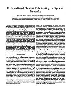
Fig. 1. A hub tree. A “region” of terminals is represented by a dashed circle. Internal black nodes of the tree are the ones that will be mapped to hubs in the network topology. White leaf nodes are terminals.

B. The Hierarchical Hub Routing Template (HH) We make heavy use of the generalization HH [15]. Such oblivious routing templates are derived from a tree T whose leaves consist of the terminal nodes, that is V (G) without loss of generality. We call this the hub tree. The internal nodes are “abstract” in the sense that they represent nodes (yet to be identified in G) which will act as hubs for certain subsets of terminal nodes. For instance, for any non-leaf node v ∈ T , let Tv be the subtree rooted at v dangling below it. The interpretation is that the leaves Lv in Tv represent a region of terminal nodes which should have a dedicated hub (this hub will correspond to v). The family of regions arising from a tree obviously forms a nested family (Figure 1). Obtaining an oblivious routing template from the HH class is a two step process. First, we first need to pick a hub tree, and then map its internal node to physical nodes. In this second stage, we find a map from each internal node v to a real node in G to act as a hub. Such a hub map η : V (T ) → V (G) must satisfy η(v) = v for each leaf of T . Given such a mapping, there is an induced oblivious routing template defined as follows: for each pair of leaf nodes i, j in T , let i = v0 , v1 , v2 , . . . , vl = j be the unique ij path in T . For each q = 0, 1, . . . , l − 1, let Pq denote a shortest η(vq )η(vq+1 ) path in G. Then we define Pij to be the concatenation of paths P0 , P1 , . . . , Pl−1 (resulting in a possibly non-simple path). Naturally, the special case of HUB routings corresponds to taking T equal to a star. Each hub tree thus gives rise to many possible routing templates, one for each mapping η (analogous to the specific choice of hub node in hub routing). Call this the class of hierarchical hub templates. Note that, in some scenarios, there are single-path oblivious routing templates that are unachievable by hierarchical hub templates. For instance in a complete graph on four nodes, with unit weight edges, there is no hierarchical hub template which corresponds to the shortest path template (each Pij consist of the edge ij). HH routing also responds to one practical impediment of hub routing architectures, pointed out in [3]. Namely, network providers are generally opposed to having all traffic routed via a single hub (or a small cluster of hubs) in the center of a large network. In particular, traffic within some local region should be handled by hubs within their own “jurisdiction”.

5

Hub trees potentially give a mechanism for specifying these local jurisdictions. IV. T HE O PTIMIZATION P ROBLEM RNDHH There are several layers to the optimization problem RNDHH . First, we must find a hub tree T - this is the core decision for which we provide a heuristic algorithm in Section IV-A. Second, given a hub tree, we must map it to the network graph to obtain a valid routing template. An efficient solution to this mapping problem is known for T -topes4 [15]; we show that this can be invoked to solve the problem for general polytopes in Section IV-B. Finally, given a template, we must ultimately solve for capacities it induces, as we discuss in Equation (2) below. We mention that the case where the hub tree is given is of interest in cases where a network provider wishes to self-identify a regional clustering within their network. In other words, they provide the hub tree, and it only remains to identify which nodes to act as hubs (i.e. solve the hub placement problem). In Section IV-C we discuss several classical problems which arise as special cases of RNDHH . Finally, we provide some theoretical bounds between RNDHH and RNDSP in Section IV-D. A. Choosing the Hub Tree We now develop a heuristic for RNDHH . It is tailored for the capped hose model, but could be extended to handle any traffic polytope. The high-level intuition is to group nodes so that traffic within a group is large compared to traffic leaving the group. This suggests the need for a hub to handle the group’s local traffic. It is straightforward to show that there is always an optimal hub tree for RNDHH where the tree is binary (we defer the details to the end of this section). Hence our algorithm’s focus is to find a “good” binary hub tree. To construct a binary tree from the terminal nodes V , one could either proceed by a top-down approach (recursively splitting groups of nodes in two) or a bottom-up approach (recursively merging nodes together). The former has the flavour of repeatedly solving S PARSEST C UT problems. This problem is APX-hard and the current best approximation factors are polylogarithmic [20], [21]. Instead, we follow the bottom-up approach. We are thus seeking to repeatedly merge pairs of node sets which share a lot of traffic with each other. The key to this calculation is a sparsest cut-like measure which we introduce next. This is then used in a Binary Tree Sparsest Merging (BTSM) algorithm. A SPARSITY MEASURE We devise a sparsity measure that seeks to maximize the traffic between two groups, compared to the traffic sent outside the merged groups. This measure is very similar to the capacity on a fundamental cut explained in Section III-A. 4 A T -tope is a polytope of demands, denoted by H T,b , which are routable on some tree T with edge capacities b. This class generalizes hose polytopes, which can be viewed as demands routable on a star.

In the setting of the capped hose model, the maximum possible demand between a pair of disjoint sets of nodes A, B ⊆ V is given by P u∗ (A, B) = maximize i∈A,j∈B Dij subject to D Pij ≤ Uij for all i, j for all i . j Dij ≤ U (i) Dii = 0 for all i D≥0 This problem can be solved efficiently, since it can be cast as a b-matching or max-flow problem. For instance, consider a bipartite graph H with bipartition A, B. Each edge ij has a capacity of Uij and is oriented from A to B. We also add a source s with edges (s, i) for i ∈ A with capacity U (i). Similarly we add sink t with edges from B. A max st-flow in this graph gives precisely the value u∗ (A, B). The sparsity of a pair of disjoint sets of nodes A, B ⊆ V is then: u∗ (A ∪ B, V \ (A ∪ B)) . sc(A, B) = u∗ (A, B) One notes that it trades off the flow out of A ∪ B versus the flow between A, B. T HE S PARSEST M ERGING A LGORITHM Our proposed heuristic algorithm (see Algorithm 1) builds up a binary hub tree T , starting from a forest consisting of a set of singletons. At each step it has a forest and looks for a pair of rooted trees that has the minimum sparsity value. Specifically, it computes the sparsity measure for the leaf sets for such a pair of trees. The two subtrees are then merged, that is, a new root node is added to T and becomes the parent of the two previous rooted subtrees. When the forest becomes a single tree, we stop. Clearly this can be done in polytime. Algorithm 1 Binary Tree with Sparsest Merging algorithm. Require: A set of nodes nodes V with peak demands U (i, j) for each pair of nodes i, j ∈ V and marginals U (i) for each node i ∈ V . Ensure: A binary demand tree T . T = (V, ∅) S ← V (T ) while |S| > 1 do Find i, j ∈ S that has minimum sparse cut value. Add a new node u to T . Connect u to i and j. Add u to S. Remove i and j from S end while return T R ESTRICTING TO B INARY T REES . In this section, we show that there is always a binary hub tree that is optimal for RNDHH . Let T be any hub tree that has at least one node u of degree at least four. Then it is possible to form a new hub tree T 0 with cHH (T 0 ) ≤ cHH (T ), and such that the sum of the degrees of

6

fundamental cut induced by e). If D is the demand polytope, then the maximum amount of demand across edge e is X uD,T (e) := max Dij . (2)

u0

D∈D

u

u00

Fig. 2. Dividing internal nodes to get a binary tree.

nodes with degree greater than four is smaller in T 0 . Hence, repeating the process eventually reduces the number of degree at least four nodes to zero, and we end up with a binary tree. Consider a u of T with degree at least four. Replace u by two nodes u0 and u00 such that u’s old parent is now connected to u0 , and u0 is connected to u’s first child as well as to u00 . Then u00 is connected to the remaining children of u (see Figure 2). Note that the sum of degrees of nodes with degree at least four is decreased by one, since u0 has degree three and u00 has degree deg(u) − 1. The capacity on the edge between u’s parent and u0 is equal to the capacity between u and its parent; the capacity between u0 and u00 can be inferred using equation (2). All other capacities remain the same - the capacity between one of u’s children and its new parent u0 or u00 is the same as the capacity between u and that child in T . Note that we only split u into two nodes and added enough capacity between those two nodes to route any feasible traffic matrix. Hence we have the new capacitated T 0 can support exactly the same demand matrices as T (i.e. the T 0 -tope and T -topes are the same). Finally, an optimal hub map of T can be implemented for T 0 as follows. One maps u0 and u00 to the node that u is mapped to. Hence, T 0 can produce the same oblivious routing as T , so its optimal cost cHH (T 0 ) is at most cHH (T ). B. The Hub Placement Problem Suppose we are given a network graph G, hub tree T with leaf set V (G) and edge capacities u. In [15], a dynamic programming algorithm is given to find a valid mapping η : V (T ) → V (G) which minimizes the hub tree’s capacity P routing cost cHH (T ) = u(e)dist G (η(w), η(v)), e=wv∈T where distG (s, t) is the length of a shortest st-path in G with edge costs c. We now describe how this is used for general hub placement in RNDHH (G, c, D). Consider any demand between i, j. If e = wv lies on the unique ij path in T , then this demand ultimately routes on a shortest path between η(w), η(v) in G. Hence if there are demand matrices that route X units of flow on e in T , then we need to reserve X units of capacity on a (presumably shortest) η(w)η(v) path in G. In other words, the RNDHH hub placement problem reduces to the dynamic program mentioned above where the u(e) values are the solution to the following problem: here, for e ∈ T , fund(e) denotes all terminal pairs i, j whose path in T uses edge e (i and j are separated by the

i,j∈fund(e)

Thus a tree T plus the polytope D induce some maximum capacities on the edges in T . These represent how much capacity we need to install on each “shortest path η(w)η(v)” to route D. These in turn drive the dynamic program for placing the hubs. Note that we have chosen uD,T to be the smallest capacity vector u such that D ⊆ HT,u . In other words, designing a network to support the T -tope HT,uD,T also supports D. Under an arbitrary mapping η : V (T ) → V (G), we must reserve uD,T (e = vw) units of capacity for the circuit on the shortest path between η(v), η(w) in G. Hence the triple T, D, η induces a total capacity cost of X cHH (T ) = uD,T (e)distG (η(v)η(w)). (3) e=uv∈T

We refer to the hub placement problem as determining the map η which minimizes (3). In [15] a dynamic programming algorithm is given to find the optimal mapping efficiently. This forms the basis of their O(1)-approximation for the Generalized VPN Problem. Namely, the general RND problem for T -topes. C. RNDHH and Other Algorithmic Problems RNDHH contains well-studied algorithmic problems as special cases. First, if D = HU is the class of hose matrices, then, as mentioned earlier, an optimal solution to RND is induced by a hub routing template, which is in turn induced by a star hub tree. Hence in this case RNDHH = RNDHUB = RND. Second, consider the case where D consists of a single demand matrix D. Obviously, the optimal solution is induced by a SP template. RNDHH however, asks for an optimal HH templates. This is a classical problem in combinatorial optimization called the minimum communication cost tree (MCT). Find some tree (not necessarily in G), containing V (G), such that if we route the demands D on T , the overall routing cost is minimized.5 Being allowed to use a hub tree for the routing, as opposed to a subtree of G, essentially means that we are restricting to MCT with metric costs6 . For the special case where G is itself a complete graph with unit-cost edges, Hu [23] showed that an optimal solution is induced by a so-called Gomory-Hu tree on the complete graph with edge capacities Dij .7 As we now see, RNDHH may incur a logarithmic increase over RND, and in fact RNDSP . On the positive side, it is known that in general there is a tree in the metric completion of G whose “distortion” is at most O(log n) [24]. The approach of Gupta thus yields an O(log n) approximation for RNDHH . 5 This

is directly related in turn to the average stretch tree problem [22]. are metric if they are induced by a cost function that is a metric. 7 In general, the Gomory-Hu tree for a capacitated graph need not be subtree of the graph; hence the requirement that G is complete. 6 Costs

7

One can see this by noting that RNDHH costs no more than a best tree routing on T in the metric completion. To see this, define a hub tree T 0 by hanging a leaf edge vv 0 from each node of T . Then consider the mapping where each v, v 0 maps to v ∈ G. This establishes: Fact 1. For any instance of RND, RNDHH ≤ RNDTR . While these techniques yield an O(log n)-approximation for RNDHH and hence also MCT, it cannot be ruled out that there are polytime O(1)-approximations. For the purposes of our study, we use a heuristic algorithm instead of metric embeddings. This is outlined in Section IV-A. D. Basic Results for RNDHH In this section we show that RNDSP and RNDHH are incomparable; depending on the instance, one may be significantly cheaper than the other. This motivates our main goal of classifying the demand spaces according to which template is better. We now establish a family of RND instances where RNDHH does much worse than RND, and in fact worse than RNDSP . Theorem 1. There is a sequence of (unit-cost) graphs {Gn }n∈N on n nodes and demand polytopes {Dn }n∈N such that for these instances RNDHH (Gn ) = Ω(log n RNDSP (Gn )). Proof. We describe G = Gn and P = Pn for a fixed n. The network graph G consists of a d-regular, α-expander graph on n vertices, where d = O(1) and α = Ω(1) (see [25] for existence proof). Directly we have that |E(G)| = O(n). Moreover, all edges have unit cost. The demand polytope D consists of a single matrix: one unit of demand between the endpoints of any edge in G. The RNDSP solution then consists of the network itself (route each demand on its own edge). Its cost is O(n), the number of edges in the graph. Let T be any hub tree. We show that the cost of any HH solution induced by T is Ω(n log n). Hence, RNDHH is Ω(n log n). Let c ∈ V (T ) be a center of the tree, that is each component of T \ {c} has at most n2 leaves (it is well-known, and easy to see that every tree has a center). We call an edge e ∈ E(G) separated by c in T if its endpoints lie in different components of T \{c}. We let Ec ⊆ E(G) be the set of all edges separated by c in T . Let Ci be one of the components in T \ {c} and let `(Ci ) be the leaves of Ci . We know that |`(Ci )| ≤ n2 . Hence, since G is an α-expander, there is at least α|`(Ci )| edges going out of Ci . So we have that |Ec | (or the total number of edges between the Ci ’s) is at least 1X αX αn |Ec | ≥ α|`(Ci )| = |`(Ci )| = 2 i 2 i 2 P as i |`(Ci )| = n (the leaves of T consist of the nodes of G).

Let η : V (T ) → V (G) be the optimal hub map for T . Call a node v ∈ V (G) close to c if 1 α distG (η(v) = v, η(c)) < logd (min{ , }n). 2 2d Let Vc be the set of close vertices in G. Since G is a d-regular graph, its size is bounded by 1 α 1 α |Vc | ≤ dlogd (min{ 2 , 2d }n) = min{ , }n. 2 2d We now merge the two concepts and say that an edge e = xy ∈ Ec that is separated by c in T is good if both x, y ∈ Vc , i.e. x, y are close to c. Conversely, an edge e = xy ∈ Ec is bad if one of its endpoints is not close to c in T . Let B be the set of bad edges. By the d-regularity of G, a bound on the number of bad edges is given by

αn dαn α d|Vc | ≥ − ≥ n. 2 2 4d 4 Since the bad edges are unit demands that must be simultaneously routable in T , the “non-close” endpoint of these demand edges must route through the image η(c) of c, imposing a cost of at least logd (n). We have Ω(n) bad demands, each incurring a cost of Ω(log n), and thus the cost of the optimal H IERARCHICAL H UBBING induced by T routing is Ω(n log n). |B| ≥ |Ec | −

The next result shows that RNDTR may be much cheaper than RNDSP . Hence, we can get an unbounded gap between RNDSP and RNDTR . By Fact 1, this implies that RNDHH may also be much cheaper than RNDSP . Theorem 2. There is a sequence of weighted graphs {Gn }n∈N and demand polytopes {Dn }n∈N such that RNDSP (Gn ) = Ω(n2 ) and RNDTR (Gn ) = O(1). Proof. The network G = (V, E) (actually G2n+2 ) consists of two stars centered at nodes a, b connected by an edge. The leaves are vi , vi0 with the following edges: E = {avi : 1 ≤ i ≤ n}∪ {bvi0 : 1 ≤ i ≤ n}∪ {vi vj0 : 1 ≤ i, j ≤ n}∪ {ab}. The edges are weighted as follows: the bridge edge ab has weight one, the star edges avi or bvi0 for 1 ≤ i ≤ n have 1 weight 2n and the edges vi vj0 for 1 ≤ i, j ≤ n have weight 1 1 − n. The (symmetric) demand polytope D consists of convex combinations of unit demands between vi and vj0 . That is, for each i, j let Di,j be the matrix with Dvi vj0 = Dvj0 vi = 1 and all other entries 0. Then D = conv(Di,j ). The optimal shortest path template in the network consists of routing the demand between vi and vj0 through the edge of

8

cost 1 − n1 connecting vi and vj0 . This template induces a cost of RNDSP = n2 (1 − n1 ) = n2 − n = Ω(n2 ). Now consider the tree template induces by the union of the two stars. In order to support D, the sub-optimization problem only reserves one unit of capacity on the bridge edge ab, as well as one unit on all star edges. Hence, this capacity cost is O(1), and is an upper bound for the best tree solution. V. E VALUATION S TUDIES We compare the network design costs for capped hose models using the routing strategies SP and HH. We solve the associated optimization problems (RNDSP , RNDHH ) across many instances of the capped hose traffic model. For the purposes of this study, we implemented an exact method for SP, and employed our BTSM heuristic in the case of HH routing. For the evaluation set-up, we use two carrier network topologies: the American backbone network Abilene (11 nodes, 14 edges), and the Australian telecom network Telstra [26] (104 nodes, 151 edges). We assume that per-unit link capacity costs are proportional to physical distances so we use this as our cost vector c for determining the best RND solution. Our traffic data is based both on randomly generated traffic instances within the capped hose model constraints, as well as on a traffic scenario based on real data. For the simulated traffic scenarios, for each network we randomly generate many traffic instances (each corresponding to a capped hose polytope) on which to solve RND. That is, each instance arises from some collection of peak demands and marginals. Our random instances are generated starting from actual population statistics (see Section V-A). In addition on Abilene, we use real data based on previous work from [27] which gives a time series of point-to-point demand measurements that can be used to create capped hose models (described later). Our results show that HH templates are often the most cost-effective. That is, RNDHH is very often less than both RNDSP , and RNDHUB . In particular, this means that by adding peak capacities U (i, j) into the hose model, the singlehub tree-routing template is no longer cost-effective. We need additional hubs for a cost-effective network design. This is strong evidence for the use of HH routing. A. Generating Traffic To generate our traffic demand matrices, namely marginals U (i) and peak demands U (i, j), we try to mimic how traffic is naturally generated in todays core networks. It has been widely accepted that core traffic is stochastic in nature (“bursty”) and that peak demand is much larger than average demand. This change in traffic patterns presents a moving target for service providers. The uncertainty is due to novel contentbased network applications combined with factors such as data center consolidations and content mobility (content migrating from location to location based on where they are consumed). Therefore in our evaluation scenario, we first assume peak demands, and then impose marginals based on the equipment

choice at each node (capacity and number of ports at the ingress and egress nodes). Our process is anchored by first fixing the peak demand between every pair of node locations based on their population [28]. This gravity model takes into account the population size of the two sites as well as their distance. Since larger sites attract more traffic and closer proximity can lead to greater attraction, the gravity model incorporates these two features. The relative traffic between two places is determined by multiplying the population of one city by the population of the other city, and then dividing the product by the distance between the two cities squared. In our case, the peak demand between two cities i, j is U (i, j) = α(i, j) Population(i) Population(j)

(4)

where α(i, j) = 1/distance(i, j) and distance(i, j) is the geographical distance between node i and node j. As datacenter based traffic dominates over the Internet, significant research activity is underway to learn the characteristics of this traffic. However, as noted in [29] we see that the end-to-end traffic matrix showing how the total traffic to YouTube video-servers are divided among different data centers follows the gravity model. On the other hand, the entryexit traffic matrix seen by the ISP suggests that data-center traffic flows are not getting divided to different locations. This is due to the impact of BGP routing policies employed by the ISP to handle datacenter-bound traffic. G ENERATING MARGINALS To generate marginals, we propose sampling within the individual relevance intervals, as discussed in Section II-B. We start by discretizing U (i)’s relevance interval into s > 0 steps, for each of the n nodes i. Then, for each value σi ∈ {0, 1, 2 . . . , s} we get a U (i) within its relevance intervals. Formally: σi X U (i, j) − max U (i, j)). U (i) = max U (i, j) + ( j j s j Thus each vector σ ∈ {0, 1, . . . , s}n yields an instantiation of the marginals. For fixed s and n, this gives (s + 1)n possible data points, yielding all possible marginals within their relevance interval up to a precision based on the coarseness of the discretization (size of s). It is impractical to generate all (s + 1)n points for large n and s. To bypass this, we use a smaller value k in place of n to generate (s + 1)k points. We then sample uniformly from these σ to assign the values for each node, i.e. we mimic the distribution of the short vector σ of length k to create our longer marginal vector of length n. So we get σU [k] X U (i) = max U (i, j) + ( U (i, j) − max U (i, j)). (5) j j s j where σ ∈ {0, 1, . . . , s}k and U[k] is chosen uniformly at random from {1, 2, . . . , k}. B. Time-Series Traffic Matrix Data For the Abilene network, we use the estimation of pointto-point demands from the work of [27] to create a realistic

9

i1 i3

i2 e s

... t

i2k+1 Fig. 3. Going from ij to ij+1 , always through e = st and along shortest paths.

data point. The data consists of 24 weeks worth of traffic matrices sampled each five minutes. In other words, we get t }Tt=1 (T = 48384) of demands from i to a sequence {Di,j j for all nodes i, j in the network. We transform this data into marginals and peak demands for a capped hose model as follows. The peak demand between two nodes i, j is by t definition U (i, j) = maxt Di,j . Similarly, node i’s marginal is the (minimum) capacity required to route the maximum P traffic t out of that node at a given time step: U (i) = maxt j Di,j . We consider different sampling intervals, i.e. various T ’s. C. Computation of Link Costs It is simple to compute the capacity u(e) needed on each edge e for HH - we just add up the capacities from every hub tree edge f = ij for which the η(i)η(j)-path passes through e. For SP, we follow a similar sub-optimization as used for HH P templates. Namely, we find the maximum value of u(e) = ij wij (e)Dij over all demand matrices D in our capped hose universe D where wij (e) is 1 if Pij uses edge e, and is 0 otherwise. For any edge e = st, it is straightforward to see that the set of ij’s with wij (e) = 1 induces a bipartite graph H = (V (G), {ij : wij = 1}) when the Pij ’s are shortest paths. Suppose H is not bipartite, then there is an odd cycle C = i1 i2 . . . i2k+1 . Thus, wi2k+1 i1 = 1 and wij ij+1 = 1 for all 1 ≤ j ≤ 2k + 1. Without loss of generality, the fact that Pij ’s are shortest paths implies that ij is closer to s for odd j’s and closer t for even j’s (see Figure 3). But then this means the path Pi02k+1 i1 = SPG (i2k+1 , s) ∪ SPG (s, i1 ) is strictly shorter than Pi2k+1 ,i1 as it doesn’t use e; contradiction. Hence we may use a max flow routing algorithm to compute u(e). The computation of link capacities can thus be done with a collection of all shortest paths {Pij } generated using standard algorithms. Algorithm 2 illustrates our experimental procedure. D. Results In Figures 2 and 3, we plot the results of the low-cost routing templates for two different network topologies Abilene and Telstra8 . Traffic matrix instances are plotted according to their marginal and peak demand strengths and coloured based on the ratio between the edge cost of the (optimal) SP routing template and the HH routing template. A blue point indicates that SP is better and a red point indicates that HH is better. 8 A much smaller number of points were sampled to cover most of the spectrum due to the computational constraints caused by the size of the Telstra network.

Algorithm 2 Experimental procedure. Require: Network graph G = (V, E) (where edge costs correspond to the geographical distance between edge’s endpoints) and parameters s, k ∈ N. for each pair of node cities i, j ∈ V do Fix point-to-point peak demand between i and j as per Equation (4). end for for each σ ∈ (s + 1)k do for each i ∈ V do Fix node i’s marginal as per Equation (5). end for This gives a capped hose model cH arising from marginals U (i)’s and peak demands U (i, j)’s. Find marginal strength vector µ of cH. Find peak demand strength vector π of cH. Solve RNDSP (G, cH) optimally. Use our BTSM heuristic and Olver et al’s algorithm [15] to approximately solve RNDHH (G, cH) and get a solution of cost RND0HH (G, cH). RNDSP (G,cH) . Report kµk2 , kπk2 and RND 0 HH (G,cH) end for

Moreover, the intensity of the colouring is proportional to the proximity of the ratio to one. If the costs of SP and HH are very similar, the color is almost white, otherwise it is highly saturated Intuitively, and as discussed in Section II-C, the x-axis corresponds to the affinity of the traffic to the hose model. A large µ value means more constraining marginals. Thus the optimal routing should primarily consider the marginals only. So we expect hub routing to do much better. Similarly, the y-axis corresponds to the affinity of the traffic to the peak-demand model. Again, a large π value means more constraining peak demands, and thus we expect SP to do much better. Furthermore, there is a duality between the µ and π values: a demand universe can only have strong marginals or strong peak demands, not both. This explains the quarter circle “swoosh” shape of the plot. VI. D ISCUSSION In [3], hub routing was used to compare the cost of two architectures: one based on IP routing and one employing circuits. Our work focuses on how the link and/or node costs vary with the choice of routing template. We now address some of the issues and our findings. A. µ − π as indicators for the choice of a routing template We see that there is a continuum of routing templates from HH to SP if viewed as a function of the newly introduced µ and π measures. As such we propose that it is possible to define a routing indicator that accounts for the strengths of the marginals and peak demands and use this information to choose the appropriate routing template. This is an important

10

TABLE I N UMBER OF I NSTANCES WHERE HH O UTPERFORMS SP Network Abilene (total number of instances: 6561) Telstra (total number of instances: 353)

Fig. 4. The ratio between the edge cost of the (optimal) SP routing and the HH routing found with our heuristic plotted against the norms of the peak demand and marginal strength vectors for varying traffic, and the Abilene network. Data points from the time-series of traffic matrices added, with duration considered as label. Better viewed in color.

HH Optimal Multiple Hubs 3045 246

HH Optimal Single Hub 8 0

such data point comes from a compilation of the real traffic matrices over a certain period of time, as labelled next to the points. As the interval increases from one week to four, we see the capped hose model shift toward a more hose-like universe, with stronger marginal (and consequently weaker peak demands). If samples are over a short time horizon, then the demand matrix does not change significantly and as such we are designing for a single demand. In this scenario, SP yields the cheapest routing template. However as the time horizon gets longer, the different demand matrices could be significantly different and in such scenarios the more flexible design of HH/VPN brings in the added cost benefits. B. Single versus Multi Hub Routing Templates An interesting observation of this study is that there are significant cost benefits for using a multi-hub routing template versus the single-hub templates which yield optimal VPNs. Table I shows the number of traffic instances where HH is more cost effective than a single hub VPN solution. It is straightforward to see that a best solution induced by any hub tree is always as good (in terms of total cost) as a singlehub routing. Indeed, mapping all internal nodes of a hub tree to a single network node is always a valid hub placement that yields the single-hub VPN-like routing. Since the hub placement algorithm [15] is optimal, it is guaranteed to find a hub placement that is as good as the best single-hub routing. C. Routing Costs and Impact on Network Design

Fig. 5. The ratio between the edge cost of the (optimal) SP routing and the HH routing found with our heuristic plotted against the norms of the peak demand and marginal strength vectors for varying traffic, and the Telstra network. Better viewed in color.

observation because it suggests a new strategy for service providers faced with designing for changing demands. In addition to just using marginal demands, they can sample the demand space to determine the relative strengths of the peak and marginal demands. They may use this to choose an initial routing template and if necessary, evolve the template to obtain/maintain cost-efficient routing. This further justifies the need to measure link level traffic, both peak and average demand, since it can feedback into the selection of an optimal routing template for a given network topology. An important consideration is the sampling interval. The impact of the sampling interval can be clearly seen by the evolution of the real data points in Figures 4 and 5. Each

We evaluate the cost-effectiveness of the HH template against SP using both link and node costs. Link or edge capacity costs for HH are computed by solving a maximization problem over the universe of traffic matrices. For node costs we use the maximum possible link capacities that are incident on a particular node. The intuition behind using these maximum incident capacities is based on the hardware port requirements for routing/switching the total traffic through that node. However it is very rare for the all incident links at the node to simultaneously carry their maximum allowable traffic rates. From Figures 4 and 6 for link and node costs respectively, we see that HH shows significant cost savings for link costs since we take advantage of dense traffic sharing points through appropriate location of hub nodes. However, since the node costs are being evaluated using physical link capacities the gains are not as significant. VII. C ONCLUSION The capped hose model introduced in this paper shines light on the applicability of current routing template archetypes

11

Fig. 6. The ratio between the node cost of the (optimal) SP routing and the HH routing found with our heuristic plotted against the norms of the peak demand and marginal strength vectors for varying traffic, and the Abilene network. Data points from the time-series of traffic matrices added, with duration considered as label. Better viewed in color.

(HUB and SP) parametrized by the marginal and peak demands of the given traffic matrices. We have shown that using the capped hose model provides additional flexibility to network engineers for cost-optimal network design and shows the relevance of the newly introduced HH templates. In particular, this means that by adding peak capacities U (i, j) into the hose model, the single-hub tree routing template is no longer cost-effective. Moreover, the peak demand and marginal strengths presented here are a first attempt at choosing routing templates based solely on traffic information. Finally, the RNDHH problem is of theoretical interest by itself, encompassing many other well-known algorithmic problems, and is open to further investigation. R EFERENCES [1] N. Duffield, P. Goyal, A. Greenberg, P. Mishra, K. Ramakrishnan, and J. Van der Merwe, “Resource management with hoses: point-tocloud services for virtual private networks,” IEEE/ACM Transactions on Networking (TON), vol. 10, no. 5, p. 692, 2002. [2] J. Fingerhut, S. Suri, and J. Turner, “Designing least-cost nonblocking broadband networks,” Journal of Algorithms, vol. 24, no. 2, pp. 287–309, 1997. [3] F. Shepherd and P. Winzer, “Selective randomized load balancing and mesh networks with changing demands,” Journal of Optical Networking, vol. 5, no. 5, pp. 320–339, 2006. [4] R. Gao, C. Dovrolis, and E. Zegura, “Avoiding oscillations due to intelligent route control systems,” in Proc. of IEEE Infocom, 2006. [5] L. Valiant, “A scheme for fast parallel communication,” SIAM journal on computing, vol. 11, p. 350, 1982. [6] N. Goyal, N. Olver, and F. Shepherd, “The VPN conjecture is true,” in Proceedings of the 40th annual ACM symposium on Theory of computing. ACM, 2008, pp. 443–450. [7] A. Gupta, J. Kleinberg, A. Kumar, R. Rastogi, and B. Yener, “Provisioning a virtual private network: a network design problem for multicommodity flow,” in Proceedings of the thirty-third annual ACM symposium on Theory of computing. ACM, 2001, pp. 389–398. [8] D. Mitra and R. Cieslak, “Randomized parallel communications on an extension of the omega network,” Journal of the ACM (JACM), vol. 34, no. 4, pp. 802–824, 1987.

[9] I. Widjaja and A. Elwalid, “Exploiting parallelism to boost data-path rate in high-speed IP/MPLS networking,” in IEEE INFOCOM, vol. 1. Citeseer, 2003, pp. 566–575. [10] I. Keslassy, S. Chuang, K. Yu, D. Miller, M. Horowitz, O. Solgaard, and N. McKeown, “Scaling Internet routers using optics,” in Proceedings of the 2003 conference on Applications, technologies, architectures, and protocols for computer communications. ACM, 2003, p. 200. [11] M. Kodialam, T. Lakshman, and S. Sengupta, “Efficient and robust routing of highly variable traffic,” in HotNets III, 2004, p. 15. [12] R. Zhang-Shen and N. McKeown, “Designing a predictable Internet backbone network,” in HotNets III, 2004. [13] H. R¨acke, “Minimizing congestion in general networks,” in Foundations of Computer Science, 2002. Proceedings. The 43rd Annual IEEE Symposium on, 2002. [14] A. Gupta, A. Kumar, M. Pal, and T. Roughgarden, “Approximation via cost sharing: Simpler and better approximation algorithms for network design,” Journal of the ACM (JACM), vol. 54, no. 3, p. 11, 2007. [15] N. Olver and F. B. Shepherd, “Approximability of robust network design,” in Proceedings of the ACM-SIAM Symposium on Discrete Algorithms (SODA), 2010. [16] F. Grandoni, V. Kaibel, G. Oriolo, and M. Skutella, “A short proof of the vpn tree routing conjecture on ring networks,” Operations Research Letters, 2007. [17] M. Ghobadi, S. Ganti, and G. Shoja, “Resource optimization algorithms for virtual private networks using the hose model,” Computer Networks, vol. 52, no. 16, pp. 3130–3147, 2008. [18] A. Kumar, R. Rastogi, A. Silberschatz, and B. Yener, “Algorithms for provisioning virtual private networks in the hose model,” ACM SIGCOMM Computer Communication Review, vol. 31, no. 4, pp. 135– 146, 2001. [19] N. Goyal, N. Olver, and F. Shepherd, “Dynamic vs. Oblivious Routing in Network Design,” Algorithms-ESA 2009, pp. 277–288, 2009. [20] S. Chawla, R. Krauthgamer, R. Kumar, R. Yuval, and D. Sivakumar, “On the hardness of approximating multicut and sparsest-cut,” Computational Complexity, vol. 15, pp. 94–114, 2006. [21] S. Arora, S. Rao, and U. Vazirani, “Expander flows, geometric embeddings and graph partitioning,” Journal of the ACM (JACM), vol. 56, no. 2, p. 5, 2009. [22] D. Peleg and E. Reshef, “Deterministic polylog approximation for minimum communication spanning trees (extended abstract),” Automata, Languages and Programming, p. 670, 1998. [23] T. Hu, “Optimum communication spanning trees,” SIAM Journal on Computing, vol. 3, no. 3, pp. 188–195, 1974. [Online]. Available: http://link.aip.org/link/?SMJ/3/188/1 [24] J. Fakcharoenphol, S. Rao, and K. Talwar, “A tight bound on approximating arbitrary metrics by tree metrics,” in Proceedings of the thirtyfifth annual ACM symposium on Theory of computing. ACM, 2003, pp. 448–455. [25] S. Hoory, N. Linial, and A. Wigderson, “Expander graphs and their applications,” Bull. Amer. Math. Soc. (N.S, vol. 43, pp. 439–561, 2006. [26] N. Spring, R. Mahajan, and D. Wetherall, “Measuring isp topologies with rocketfuel,” SIGCOMM Comput. Commun. Rev., vol. 32, no. 4, pp. 133–145, Aug. 2002. [Online]. Available: http://doi.acm.org/10. 1145/964725.633039 [27] Y. Zhang, M. Roughan, N. Duffield, and A. Greenberg, “Fast accurate computation of large-scale ip traffic matrices from link loads,” in Proceedings of the 2003 ACM SIGMETRICS international conference on Measurement and modeling of computer systems, ser. SIGMETRICS ’03. New York, NY, USA: ACM, 2003, pp. 206–217. [Online]. Available: http://doi.acm.org/10.1145/781027.781053 [28] H. Chang, M. Roughan, S. Uhlig, D. Alderson, and W. Willinger, “The many facets of internet topology and traffic,” Networks and Heterogeneous Media, 2006. [29] V. Adhikari, S. Jain, and Z. Zhang, “Youtube traffic dynamics and its interplay with a tier-1 isp: an isp perspective,” in Proceedings of the 10th annual conference on Internet measurement, 2010.